 Mhd. Suhyb Salama
 Lazaros Spaias2
 Steef Peters
- 1Department of Water Resources, ITC Faculty, University of Twente, Enschede, Netherlands
- 2Water Insight, Wageningen, Netherlands
- 3German Aerospace Center, Cologne, Germany
It is common in estuarine waters to place fixed monitoring stations, with the advantages of easy maintenance and continuous measurements. These two features make fixed monitoring stations indispensable for understanding the optical complexity of estuarine waters and enable an improved quantification of uncertainties in satellite-derived water quality variables. However, comparing the point-scale measurements of stationary monitoring systems to time-snapshots of satellite pixels suffers from additional uncertainties related to temporal/spatial discrepancies. This research presents a method for validating satellite-derived water quality variables with the continuous measurements of a fixed monitoring station in the Ems Dollard estuary on the Dutch-German borders. The method has two steps; first, similar in-situ measurements are grouped. Second, satellite observations are upscaled to match these point measurements in time and spatial scales. The upscaling approach was based on harmonizing the probability distribution functions of satellite observations and in-situ measurements using the first and second moments. The fixed station provided a continuous record of data on suspended particulate matter (SPM) and chlorophyll-a (Chl-a) concentrations at 1 min intervals for 1 year (2016–2017). Satellite observations were provided by Sentinel-2 (MultiSpectral Instrument, S2-MSI) and Sentinel-3 (Ocean and Land Color Instrument, S3-OLCI) sensors for the same location and time of in-situ measurements. Compared to traditional validation procedures, the proposed method has improved the overall fit and produced valuable information on the ranges of goodness-of-fit measures (slope, intercept, correlation coefficient, and normalized root-mean-square deviation). The correlation coefficient between measured and derived SPM concentrations has improved from 0.16 to 0.52 for S2-MSI and 0.14 to 0.84 for S3-OLCI. For the Chl-a matchup, the improvement was from 0.26 to 0.82 and from 0.14 to 0.63 for S2-MSI and S3-OLCI, respectively. The uncertainty in the derived SPM and Chl-a concentrations was reduced by 30 and 23% for S2-SMI and by 28 and 16% for S3-OLCI. The high correlation and reduced uncertainty signify that the matchup pairs are observing the same fluctuations in the measured variable. These new goodness-of-fit measures correspond to the results of the performed sensitivity analysis, previous literature, and reflect the inherent accuracy of the applied derivation model.
1 Introduction
With the planned launch of the Pre-Aerosol Clouds and ocean Ecosystem (PACE) in 2022, and the data streaming from the Sentinel missions, Earth Observation (EO) technology is moving toward a long-term sustainable data flow, forming the basis for its operational use (Groom et al., 2019). Setting up satellite-based services for water quality monitoring in turbid estuaries provides an instrument for early warning and mitigation on extended spatiotemporal scales (Anderson et al., 2017). However, the added value of satellite products in estuarine waters is determined, primarily, by their accuracy, which needs to be validated against reference data. In this regard, continuous data measured from a fixed monitoring station are indispensable for understanding estuarine systems (Benway et al., 2019) and quantifying the uncertainties of satellite products of water quality. Validation is the action of checking or proving the validity or accuracy of satellite products. It measures the correctness and meaningfulness of derived values against measured quantities (e.g., Salama et al., 2012). In this respect, validation outputs are metrics measuring the resemblance between satellite-derived products and measured values and a set of logical values addressing whether satellite products are acceptable (Seegers et al., 2018; Werdell et al., 2018). The standard procedure of comparing point-scale measurements to time-snapshots of satellite pixels suffers from additional uncertainties related to the temporal and spatial mismatches (Evers-King et al., 2017). For example, Salama and Su (2011) have shown that the spatial mismatch between 300 and 1000 m pixel resolutions could be up to 0.02 sr−1 for ocean color remote sensing reflectance at 665 nm. From this, atmospheric correction accounts for up to 40% of the total uncertainty, which is partly due to the unavailability of information on atmospheric variables, e.g., aerosols optical thickness (Frouin et al., 2019), at the satellite measured scales. Having fine spatial resolution could provide extra details (Vanhellemont and Ruddick, 2014). However, there is a trade-off between gaining information from reducing the spatial scale and adding additional noise-component resulting from small-scale turbulences of water constituents (Bissett et al., 2004). For example, Groetsch et al. (2014, 2016) have shown a mismatch between fluorescence measurements from ship-of-opportunity, taken at 5 m below the water surface, and satellite-derived concentrations of chlorophyll-a (Chl-a). The authors attributed this mismatch to the different sample sizes of a satellite pixel vs. a point in-situ measurement and the depth-integrated satellite observation vs. in-situ measurement taken at a specific depth.
The spatial and temporal dynamics of water quality variables are particularly high in estuarine waters (Hommersom et al., 2009; Nechad et al., 2015). The spatial variability is usually addressed through assessing the homogeneity of satellite pixels of the matchup location (e.g., Harding Jr et al., 2005) or using Bayesian inference (e.g., Salama and Su, 2010). Whereas the temporal variability of in-situ measurements is usually addressed by averaging data points within a temporal window of 1 to 4 h of the satellite overpass (IOCCG, 2019). Current guidelines (e.g., Sentinel three Validation Team S3VT) minimize the spatiotemporal variability by sampling homogeneous water within ±1 h of the satellite overpass and under good atmospheric conditions. Applying these approaches to address the spatiotemporal mismatch could, nonetheless, result in variable performances and lead to little improvement in validation statistics (Barnes et al., 2019). This calls for a validation scheme that provides an unbiased assessment of uncertainty at several scales and ensures the consistency of uncertainty estimates of satellite-derived water quality variables. Recently, McKinna et al. (2021) have shown that incorporating model and observation uncertainties have improved the validation metrics. This paper incorporates the variabilities of field measurements and satellite observations to estimate the underlying accuracy of satellite-derived concentrations of suspended particulate matter (SPM) and alga’s green pigment, chlorophyll-a (Chl-a) in estuarine waters. To achieve this objective, we use semi-continuous measurements from a fixed location and observations from two satellite sensors: the Multispectral Instrument on Sentinel 2 (S2-MSI) and the Ocean Land Color Instrument on Sentinel 3 (S3-OLCI).
The paper is organized as follows: first, the employed method to answer the research question is presented in Section 2, followed by a description of the study area in Section 3. Used data and preprocessing are then detailed in Section 4, followed by results (Section 5) and discussion (Section 6). The paper is finalized with a summary of findings in the conclusion section.
2 Methods
2.1 Validation
Following the ISO standard (Åhlin et al., 2014) and its implementation in the Committee On Earth Observation Satellite, validation is the process of assessing, by independent means, the quality of the data products derived from the system outputs. For such validation to be meaningful, it should be applied to matchups—which is defined (IOCCG, 2019) as pairs of measured (say 10) and satellite-derived (say y) values that have the same locations and times (±1 h) of sampling. The validation protocol (IOCCG, 2019) suggests taking several satellite pixels surrounding the location of the monitoring station. While this could be performed in open waters, it will be a challenge in fine-scale estuarine systems where proximity to land is inevitable. The approach adopted in this paper to construct the matchup is to exclude all pixels that partially cover the ground and select the nearest water pixel to the location.
Validation is carried out on the matchup dataset using type-II linear regression (Laws, 1997; IOCCG, 2006), whereby a regression line—passing through the centroid of the data μx, μy—is estimated through adjusting its slope αII and intercept βII to minimize the sum of squares of normal deviates—lines perpendicular to the regression line. Approaches other than minimizing the normal deviates exist, e.g., calculate the geometric mean of the slope from regression of y on x and x on y but they are similar. The slope measures the gain of y, i.e., how close/far the regression line is from unity. Whereas the intercept measures the offset of y, i.e., how close/far the regression line is from passing through the origin.
In addition to the coefficients resulting from type-II regression, validation involves calculating the correlation coefficient r and the root-mean-square deviation, Δ, or the mean absolute differences (Seegers et al., 2018). The correlation coefficient, r, is a measure of linearity, whereas Δ provides the total mean uncertainty of satellite-derived products, w.r.t measured values (hereafter denoted as Δtot):
where n is the total number of matchups. Normally water authorities or engineering applications require a percentage of uncertainty to be presented from the validation of satellite products. This percentage measure is quantitative and provides an immediate feeling of accuracy. For example, most satellite missions require percentage accuracy in the derived water quality variables. The Δ could be normalized, for x ≠ 0, as (e.g., Hieronymi et al., 2017),
However, this calculation of percentage accuracy is not symmetric resulting in higher values for y < x and lower values for y > x. For example:
To avoid such a confusion, in this paper we calculate the percentage error by dividing Δ by the mean μx:
2.2 In-Situ Measurements vs. Satellite Observations
Deriving water quality variables from satellite observations requires two main steps (Gordon and Morel, 1983; Frouin et al., 2019): atmospheric correction to retrieve the water leaving signal, and deriving water quality variables from the water leaving signal. Eventually, both steps could be combined and simultaneously carried out (e.g., Arabi et al., 2016, 2018). Water quality variables that can be derived from optical observations are those with the property of changing the visible sunlight through absorption and/or scattering (Mobley et al., 1993), namely phytoplankton pigment (here we focus on the green pigment chlorophyll-a, Chl-a), suspended particulate matter (SPM) and colored dissolved organic matter (CDOM) (Kirk, 1994). This study will focus on the first two variables, namely SPM and Chl-a concentrations.
When satellite-derived SPM and Chl-a are compared to in-situ measurements, some discrepancies arise related to differences in sampled times, depths, and water volumes. Much research (see, for example, Salama and Su, 2011; Groetsch et al., 2014, 2016; Valdés and Lomas, 2017) has shown that due to these differences, in-situ devices record small turbulences (fluctuations on a short time scale) that are undetected or averaged by the satellite’s pixel observations. This phenomenon was referred to by Oke and Sakov (2008) as the representation error. This mismatch in representation will supplement additional components to the retrieval’s uncertainty, Δtot, namely uncertainties related to temporal and spatial mismatches (IOCCG, 2019).
In an analogy to the Taylor approximation of the second moments and using the expression of Salama and Stein (2009), Salama and Su (2011), and Salama et al. (2011), the total uncertainty could be approximated as the sum of three components:
where the subscripts stand for temporal (t), spatial (s), and derivation (d) uncertainties. Eq. 3 separates the total uncertainty into three contributors: derivation, spatial, and temporal mismatch. The derivation uncertainty
2.3 Representative In-Situ Measurements
Depending on the sampling frequency of the in-situ device, n measurements will be recorded within the 2 h of the satellite overpass. Validation protocol (IOCCG, 2019) commonly advises to average in-situ measurements that fall within a temporal window of 1 to 4 h of the satellite overpass. However, due to the representation error discussed in the previous section, this time window (±1 to ±4 h) depends on water quality dynamics with spatial and temporal dependencies. To reduce representation error resulting from temporal averaging and ensure that these n measurements represent the same dynamics, we group the data based on their variability. This is done by selecting subsets that fall within a range of variabilities and recorded in a sequential (uninterrupted) timespan. This additional grouping produces sets of representative measurements (hereafter called “optimal in-situ matchup”) that fall inside satellite pixels and form the primary basis for assessing the accuracy of satellite derived water quality products, and is performed as follows:
(i) Analyze the dis/similarities between in-situ measurements;
(ii) Determine data points that have inter-variance that falls within a range of variability (will be defined later in this section);
(iii) Identify the subset from [ii] that has a sequential recording time.
The (dis-)similarities between consecutive records of in-situ measurements can be quantified by the empirical semivariogram (Bowman and Crujeiras, 2013). For the 2-h span, the empirical semivariogram can be estimated from the data points as:
where γ(x, dt) is the temporal semivariogram of x with a time lag dt and n (dt) is the number of bins (data pairs) of width dt.
Similar measurements have sequential recording time and fall within the range of data variability, say γs:
The value of γs Eq. 5 is empirically estimated in this work by employing the principle of insufficient reason (Jaynes, 1957; Salama and Shen, 2010), which states that when there is not enough evidence to separate the uncertainties in Eq. 3, we can assign uniform weights, i.e.,
The total uncertainty
With rx,y being the correlation coefficient between x and y. For standardized anomalies the condition Eq. 6 becomes:
The application of Eq. 8 requires iteration to estimate the correct value of rx,y. The iteration procedure is detailed in Section 5.2.
The semivariogram Eq. 4 and the similarity condition Eq. 8 can be applied on each data point as well (instead of one data point of the satellite overpass) producing thereby m records of similar measurements, with m being less than the number of data points within ±1 h of satellite overpass (i.e., 120). These m sets of similar measurements provide an ensemble of information to carry out the validation.
2.4 Unbiased Validation
The component Δd in Eq. 3 represents the underlying accuracy of satellite-derived water quality and should therefore be unbiased. A technique to estimate Δd without the need to calculate the individual components of Eq. 3 is described hereafter and starts with the assumption that variables x and y are normally distributed and often log-normal (Campbell, 1995).
The matchup pairs of measurements (x) and satellite-derivations (y) should in principle be linearly related in the form of
Eq. 9 means that if satellite-derived products are linearly related to measured variables, a requirement to accept derived products, their anomalies should be equal. This finding from Eq. 9 has great utilities, as it facilitates incorporating the ratio σx/σy in the validation to better estimate the derivation uncertainty, Δd. The main assumption here is that, adjusting satellite-derived values, y, such that they have the same mean and standard deviation of measured values will yield new satellite-derived values,
We start first by approximating Eq. 9 as:
Second, the values of x are substituted with new updated satellite-derived values
Rearranging the sides of Eq. 11 the new updated
From Eq. 12, it can be shown easily that
Eq. 13 demonstrates that for values of the correlation coefficient r ≥ 0.5 the Δ will always be equal or less than σx and the uncertainty cannot be larger (r → − 1) than 2σx. There is one drawback for Eq. 13, namely when r → 1 the value of uncertainty Δd will vanish. For the presented data, this condition was unlikely with the value of rx,y not exceeding 0.6.
Eq. 13 provides the minimum value of uncertainty if σy > σx, the proof is provided in the Appendix section Proof I. In addition, the slope and intercept (αII, βII) of the type-II regression between x and the updated values
3 Study Area
The method presented in Section 2 is applied to matchups in the Ems-Dollard estuary, a semi-enclosed body of water stretching from the Ems River’s Mouth to the Island of Borkum in the Wadden Sea along the Dutch-German border (Figure 1). The estuary covers an area of 1071 km2, half of which consists of intertidal flats (Compton et al., 2017). Concerning the Amsterdam Reference Level (Normaal Amsterdams Peil, NAP), the tidal channel has a depth ranging from ≈ − 1.5 m to ≈ − 25 m.
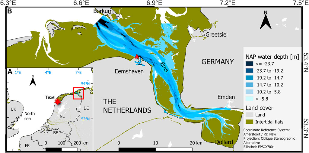
FIGURE 1. The study area: (A) locations of the Ems Dollard Estuary (red box) and the Texel station (red star); (B) bathymetry of the Ems Dollard Estuary, water quality data are obtained from the Eemshaven station (red triangle). Coastlines are from EEA (2018), Bathymetry data are from Pierik (2019), land classes are from Corine (2018).
Ensemble of physical processes, dominated by large tide gradients and freshwater influx, control the dynamics in the Ems’s estuary. The Ems Dollard is a mesotidal estuary with a semi-diurnal tidal cycle that ranges between 2 m in the channel (inner Ems) to 3 m near the mouth of the Ems River (de Jonge, 1983). The primary source of freshwater inflow is the Ems River, with a mean discharge of 100–120 m3 s−1, with a high dynamic range from 25 to 390 m3 s−1 (Ysebaert et al., 1998). Recently, Schulz et al. (2020) showed that the system alternates between a destratification state during the flood and a built-up of stratification throughout the ebb. The authors also observed that the lateral circulation experiences abrupt transitions during a tidal cycle with large spatial variabilities at fine-scale (
The high turbidity and the fine-scale variability in the Ems Dollard estuary poses a challenge for in-situ measurements and validation of satellite products. In this respect, measurements from fixed stations require careful selection to be representative of the matching satellite pixels. Details on this selection procedure are provided in Section 4.
4 Used Data
4.1 In-situ Data
For this research, we have collected in-situ and satellite data forming two sets of matchups: radiometric and water quality derivations. The in-situ data were collected from two permanent monitoring stations located at Texel Island and Eemshaven, both in the Dutch part of the Wadden Sea, about 150 km apart. The Texel station provided radiometric data for atmospheric correction, whereas the Eemshaven station provided measurements on water quality variables serving the purpose of validation.
4.1.1 Radiometric Data
Radiometric data, from proximity (i.e., close-range) remote sensing, were obtained from the permanent station at Texel Island in the Wadden Sea, the red star on Figure 1A. The Texel station has three RAMSES TriOS sensors measuring upwelling radiance and sky-radiance and downwelling irradiance covering the visible range between 318 and 950 nm at ≈ 3.3 nm spectral interval. Radiometric data and their preprocessing chain of converting to reflectance and quality check are described with great detail in Arabi et al. (2018, 2016). Proximity remote sensing data are used in this study to identify the atmospheric correction procedure most suited for the Wadden Sea. Three years of Texel data (from 2015 to 2017) that are matching satellite observations (±1 h) were averaged on the 2-h period (eight measurements) and used to establish the radiometric matchup set. Radiometric data from proximity remote sensing were transformed to the bands of the matching space-sensor using its spectral response function.
4.1.2 Water Quality Data
The Department of Public Works and Water Management (Rijkswaterstaat, RWS), have a permanent station in the Eemshaven, the red triangle in Figure 1B. This station contains a YSI 6600 V2 sensor at -3.5 m deep (NAP reference), measuring turbidity (in NTU unit) and chlorophyll-a concentration each minute of the day. Fixed monitoring stations of the RWS follow the guidelines of the OSPAR’s Joint Assessment and Monitoring Programme (JAMP). RWS carries out periodical quality checks with fluorometric measurements and yearly validation with HPLC. However, as the stratification occurs primarily during the built-up of the ebb, and the maximum turbidity is near the bottom, YSI6600 measurements during the flood cycle were selected (Schulz et al., 2020), see Section 4.3 for more details.
The conversion from NTU to g.m−3 is performed using two gain factors: 1.7 for silt (SPM particle size
4.2 Satellite Data
Satellite observations were obtained, for both stations (Texel and Eemshaven), from Sentinel-3 Ocean and Land Color Instrument (S3-OLCI) and Sentinel-2 Multi-Spectral Instrument (S2-MSI). S3-OLCI and S2-MSI images of the Ems Dollard Estuary were collected from the Copernicus Open Access Hub (Copernicus, 2019). Three years (2015–2017) of data were used to establish the radiometric matchup set for the S2-MSI. Whereas 1 year (2017) of data was used to establish the radiometric matchup set for the S3-OLCI. For both sensors 1 year, 2017, of data was used to establish the validation matchup set. Satellite pixels covering the water nearby the Texel and Eemshaven sites were then selected based on three criteria (flags):
(i) Flagged as good observations,
(ii) Flagged as cloud-free, and
(iii) Flagged as water targets.
Ancillary atmospheric data of ozone total column, wind speed, surface pressure, and air temperature were obtained from the global reanalysis data ERA-Interim (ECMWF, 2017). ERA-Interim data are updated monthly with a delay of 2 months. Therefore, the closest data in time is used to perform the atmospheric correction.
The processing chain of satellite data followed these two steps:
(1) Different atmospheric correction methods were inter-compared using a radiometric matchup set to select the procedure with the least error. For S2-MSI we applied Acolite (Vanhellemont and Ruddick, 2014, 2015), Polymer (Steinmetz et al., 2011), Case-2 Regional/Coast Color (C2RCC), and the extreme Case-2 waters (C2X) (Brockmann et al., 2016). For S3-OLCI we applied C2RCC and an alternative version of it (C2RCC-A, C. Lebreton personal communication). The Sentinel’s toolbox (SNAP) was used to process satellite data.
(2) The Nechad-705 model (Nechad et al., 2010) was employed to retrieve SPM concentrations, whereas for Chl-a the Gons model (Gons, 1999) was employed. These models were developed for regions with similar characteristics as the Ems Dollard Estuary and were employed by this study without calibration.
The standard flags of the different atmospheric correction approaches were used without adjustment, which has caused lowering the number of radiometric matchups from 14 to 7, 9, 10 and four spectra for, respectively, Acolite, C2X, C2RCC, and Polymer.
4.3 Matchups Data
The radiometric matchup set was used to select the atmospheric correction procedure with the least error and consisted of 14 and 11 pairs of in-situ measured vs. S2-MSI and S3-OLCI reflectance, respectively. On the other hand, the validation matchup set was used to validate satellite derivations of water quality variables as described in Section 2. Each pair in the validation matchup set consisted of satellite-pixels and the matching in-situ record. To guarantee that the in-situ measurements at 3.5 m depth near the Eemshaven are representative to the surface-derived satellite concentrations of SPM and Chl-a, we filtered data using two conditions based on the recent findings of Schulz et al. (2020):
(i) Select the nearest water pixel to the Eemshaven station to minimize the cross-sectional fine-scale spatial variability.
(ii) Select measurements during the flood cycle, as the water column is well mixed.
Water level data recorded by RWS at the Eemshaven station were used to filter the data.
A summary of the validation matchup set is presented in Table 1.

TABLE 1. Water quality matchups.
5 Results
5.1 Verification of Atmospheric Correction
The results from four atmospheric correction methods applied to S2-MSI (Figure 2) show that the C2X approach rendered spectra that fall within the range of measured values. Only C2X produced spectra that are within a similar range to the measured values. C2RCC, on the other hand, resulted in S2-MSI spectra with magnitudes close to those of C×2, but with a different range and variability between 665–705 nm (i.e., absorption effect of Chl-a). The least fit was obtained from Acolite and Polymer with a noticeable higher magnitude for Polymer. More quantitative goodness-of-fit measures are presented in Table 2. Slope, intercept, and R2 were estimated from type-II regression, the Δ was normalized to the mean (denoted as
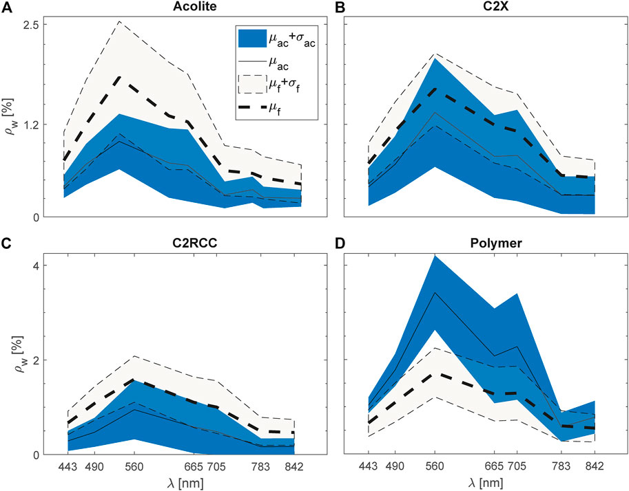
FIGURE 2. Summary of the results from applying atmospheric correction to S2-MSI using (A) Acolite, (B) C2X, (C) C2RCC and (D) Polymer. Solid lines depict average values, whereas shaded areas represent the variability as standard deviation. The subscripts, ac,f refer to atmosphere correction and field spectra, respectively.
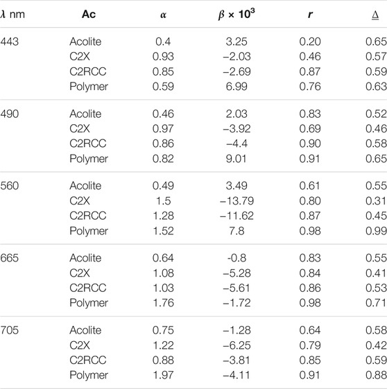
TABLE 2. Radiometric validation of atmospheric corrections applied to S2-MSI.
It is noticeable from Table 2 that Acolite and Polymer produced the least accurate results with
For the application to S3-OLCI, only the C2RCC and C2RCC-alternative were available. The results (Figure 3) show that C2RCC-alternative has a slightly better fit than its older version. More quantitative goodness-of-fit measures are presented in Table 3. Both approaches for atmospheric correction did not produce a good fit to measured spectra with very low values of correlation coefficient and large
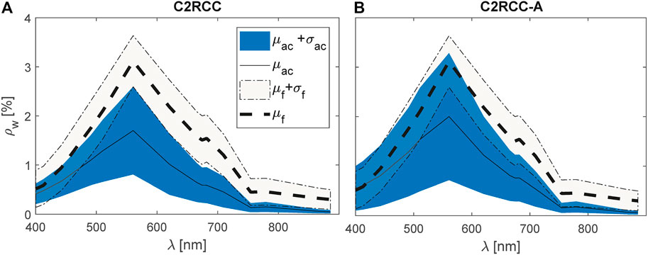
FIGURE 3. Summary of the results from applying atmospheric correction to S3-OLCI using (A) C2RCC and (B) C2RCC-A. Solid lines depict average values, whereas shaded areas represent the variability as standard deviation. The subscripts, ac,f refer to atmosphere correction and field spectra, respectively.

TABLE 3. Radiometric validation of atmospheric corrections applied to S3-OLCI.
5.2 Validation of Satellite-Derived Water Quality Variables
Figure 4 shows water quality matchups in the (±1) of the satellite overpass. This figure shows that continuous in-situ measurements contain many fluctuations that are either undetected or averaged by satellite observations. These fluctuations are large to the point that average values of satellite derivations fall outside the variability range (defined as μx ± σx) of in-situ measurements. Particularly, matchups of Chl-a values (Figure 4B,D) show larger discrepancy than the matchups of SPM (Figure 4A,C). The semivariograms of in-situ measurements are computed from the standardized anomalies and shown in Figure 5.
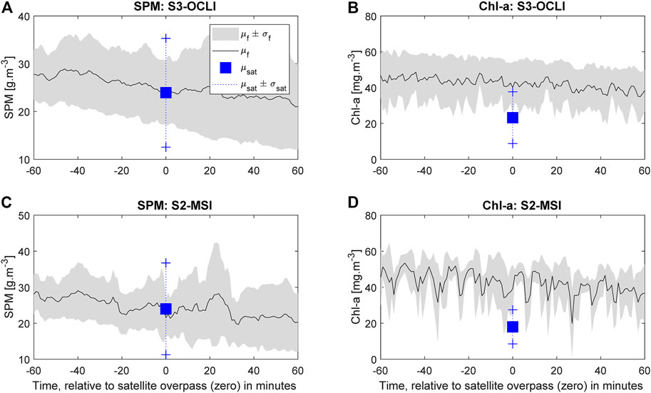
FIGURE 4. Average values and variabilities of the matchup data for S3-OLCI (A) and (B) and for S2-MSI (C) and (D). Solid lines depict average values, whereas shaded areas represent the variability as standard deviation. The subscripts, f and sat, refer to in-situ measurements and satellite-derived values.
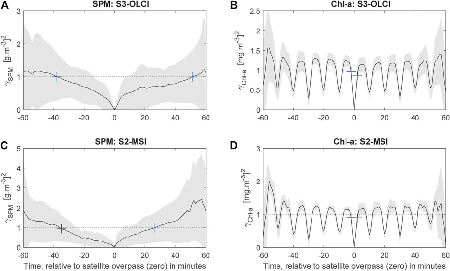
FIGURE 5. Semivariograms of in-situ measurements around the satellite overpass for S3-OLCI (A), (B) and S2-MSI (C), (D). Solid lines depict average values, whereas shaded areas represent the variability as ± standard deviation. The dotted line represents the similarity condition of Eq. 8 set to one for illustration.
To further analyze the data, we applied the extended triple collocation technique (Stoffelen, 1998; McColl et al., 2014) on the standardized anomalies of these data (see Table 4).
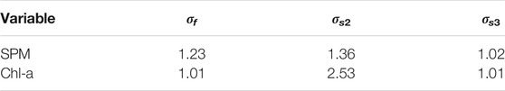
TABLE 4. Results of the triple-collocation technique applied to standardized anomalies of field measurements and satellite derived concentrations of SPM and Chl-a. With σ being the standard deviation, and the subscripts, f, s2, and s3 representing filed, S2-MSI, and S3-OLCI data, respectively.
The results in Table 4 show that the uncertainty of in-situ measurement within the ± hour of satellite overpass is comparable to the uncertainties in satellite-derived water quality products. This observation is also confirmed when analyzing the semivariograms. The semivariogram shows non-stationary and cyclic processes, particularly for Chl-a measurements, with a cycle of about 10 min. As the sensors of RWS are well maintained and periodically calibrated, this time variability could be explained by the inertial subrange (Kolmogorov et al., 1991), where phytoplankton is affected by fluctuations at a small-scale ranging from seconds to minutes. Blauw et al. (2018) measured Chl-a at 12- and 30-min intervals and found substantial hourly variations, and explained it by vertical mixing and horizontal transport of different water masses. Franks (2005) showed high patchiness (in Figure 4) of one snapshot in time of phytoplankton fluorescence taken with an imaging fluorometer. However, further research is needed to investigate this small temporal variability of Chl-a in the study area. On the other hand, SPM also shows a cyclic pattern but on a larger temporal scale of a few hours, roughly corresponding to the tidal cycle of the Ems Dollard (Blauw et al., 2012). The analysis here will be, however, focused on using the semivariograms to identify the optimal in-situ matchups. For each in-situ matchup of 120 data points, sets of similar measurements are identified by first computing the semivariograms and second applying the similarity condition of Eq. 8 using the following iterative procedure:
(i) Starting at the first data point (at t = − 60), compute the semivariogram using Eq. 4;
(ii) Initialize rx,y (either −0.995 or use the computed correlation) and compute the condition in Eq. 8;
(iii) Subset all data points that satisfy Eq. 8 and compute their median or mean.
(iv) Perform steps i to iii on all in-situ matchup and compute rx,y;
(v) Go to Step ii and replace rx,y and iterate until its value does not change significantly.
(vi) Exclude the data points that satisfy the similarity condition (say m) and move the cursor to the next data point m + 1;
(vii) Repeat Steps i to vi starting from m + 1.
Steps ii to v converge very rapidly with a maximum of eight iterations regardless of the starting value. Only sequential measurements were grouped in this similarity check. In other words, the first ms sequential data points that stratified the similarity condition were grouped. Another condition was required to guarantee that the data recorded is 5 min (i.e., five data points) or more, namely ms ≥ 5. The whole procedure, Steps i to vii, produces data records without overlap, i.e., independent, each representing a similar set of measurements. Therefore, each in-situ matchup has a different number of records. Data records with a correlation coefficient r < 0.15 were excluded from the calculation. Finally, the unbiased validation procedure of Section 2.4 is applied to the values of weighted averages Xm.
The proposed approach is compared to the standard procedure of averaging measurements within the 2-h span of satellite overpass and presented in Table 5 for S2-MSI and Table 6 for S3-OLCI.
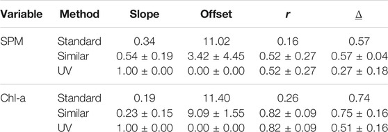
TABLE 5. Validation of S2-MSI derivations. Similar (μ ± σ) is obtained from sets of independent records of similar measurements. UV is obtained after the application of unbiased validation.
From Tables 5, 6 and Figure 6 it is apparent that using the similarity conditions of Section 2.3 to group in-situ measurements, with iterative estimation of rx,y, has improved the overall fit and produced useful information on the ranges of goodness-of-fit measures (slope, intercept, correlation coefficient, and
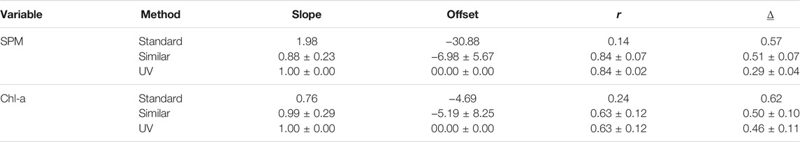
TABLE 6. Validation of S3-OLCI satellite derivations. Similar (μ ± σ) is obtained from sets of independent records of similar measurements. UV is obtained after the application of unbiased validation.
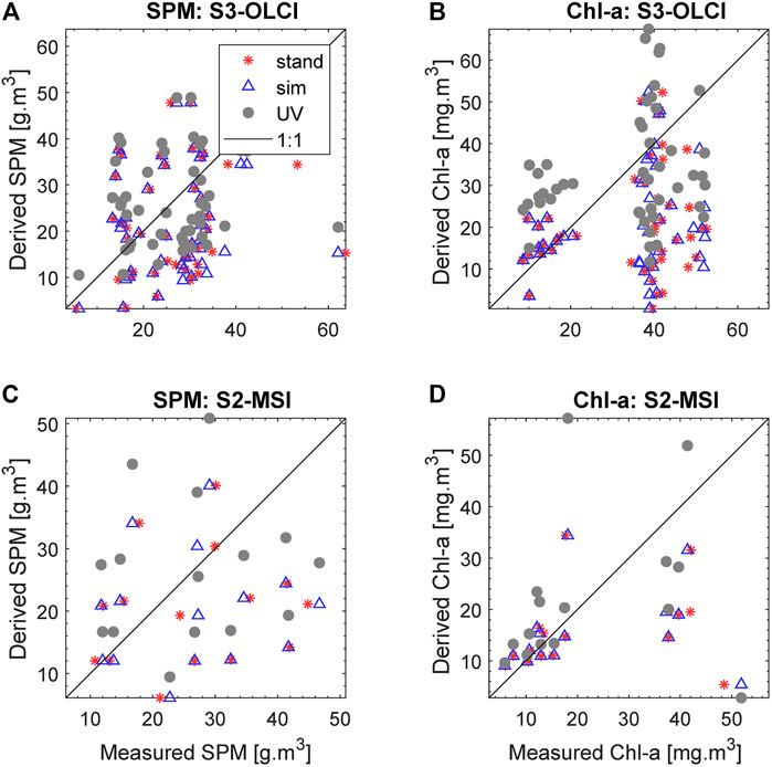
FIGURE 6. The results of the standard approach (Stand, red stars), after selecting similar measurements (Sim, blue triangles) and unbiased validation (UV, gray circles) applied to similar measurements for SPM (A,C) and Chl-a (B,D) derived from S3-OLCI (A,B) and S2-MSI (C,D).
6 Discussion
6.1 Method and Results
This study has presented a validation procedure for water quality products derived from the Sentinel missions in estuarine waters. Validation of S2-MSI and S3-OLCI products was carried out using continuous records of suspended sediment (SPM) and Chl-a measured in Ems Dollard Estuary by the Department of Public Works and Water Management (RWS) in the Netherlands. However, proximity remote sensing observations were used from the Texel station to verify the quality of atmospheric correction. From the four tested atmosphere correction approaches, C2X produced S2-MSI spectra close to measured values in magnitude and shape. For S3-OLCI, two models were available, with the augmented version of C2RCC producing slightly better results consistent with recent findings. For example, Mograne et al. (2019) compared five atmospheric correction methods for S3-OLCI over optically complex waters and found that C2RCC-A is better suited for turbid water. Toming et al. (2017) showed that C2RCC is suitable for atmospheric correction of S3-OLCI but not for deriving water quality variables. Warren et al. (2019) compared six algorithms for retrieving water-leaving reflectance from S2-MSI observations and found that all algorithms have high uncertainties, with Polymer and C2RCC achieving the lowest mean absolute differences of 40–60% in blue/green bands. Verification of atmospheric correction, although indicated radiometric accuracy, were performed far from the Ems Dollard and should, therefore, be taken with caution (Pahlevan et al., 2017; Crout et al., 2019).
In-situ data showed high variability and data points matching the satellite overpass did not correspond with satellite-derived values. This could be explained by the fact that although surface processes are related to underwater processes, this relationship is not always evident (e.g., linear/logarithmic depth profile or stratification). In this case, in-situ and satellite measurements are likely observing different processes. For example, Groetsch et al. (2014) showed that the stratification largely caused the mismatch between in-situ and satellite-derived Chl-a values during cyanobacterial blooms. Valdés and Lomas (2017) showed that turbulence of patches of water constituents are in the order of centimeters and minutes on the spatiotemporal scale, which does not correspond with satellite observations (hundred meters and snapshots). The Ems Dollard Estuary has fine-scale lateral spatial variability at fine-scale (
Each in-situ matchup consisted of 2 h measurements (one per minute), resulting in 120 data points around the satellite overpass. The semivariogram was applied to identify similar measurements: sequential and fall within a range of variability defined by the semivariogram. In applying the semivariogram and similarity condition, a different number of records for each in-situ matchup were produced with each record representing a similar set of measurements and is independent of the other records. The semivariogram was applied without exclusion to investigate the effect of records’ overlapping, i.e., staring at t = 5 and moving with an interval of 5, 23 data records for each in-situ matchup were produced. These records have some overlap, i.e., a record i could contain parts i − 1 and i + 1 records. The results, not shown here, are similar to those presented in Tables 5, 6 but with lower variability, which the overlap of the data records could explain.
The semivariogram and the similarity condition were also applied to point t = 0 around the satellite overpass but did not provide additional information as it was comparable to the standard approach. Remembering that in-situ measuring devices record fluctuations that are not necessarily observed by the satellite, and then following the principle of insufficient reason (Jaynes, 1957), any measurement, within the ±1 h of satellite overpass, could be a candidate point for selecting the optimal in-situ matchup. Using satellite estimates as background information, the concept of optimal interpolation, commonly used to grid satellite data, could be employed. We used the Cressman weights (Cressman, 1959) to produce a weighted average Xm from these m records of similar measurements:
The proposed validation procedure incorporates the variability of in-situ measurements and satellite observations (the ratio σx/σy) to estimate the accuracy of satellite-derived water quality products. Due to this incorporation, the bias will vanish (therefore, the name unbiased validation) and the validation metrics (slope, intercept, correlation, and root-mean-square deviation) will improve. Our results correspond with the recent work of McKinna et al. (2021), in which they have shown that incorporating model and observation uncertainties will improve the validation metrics. In our work, the variability of in-situ measurement σx is on a point-scale and includes two scales: 2 h (around the satellite overpass) and the time-averaged over the matchup data points. Whereas the variability of satellite observations, σy, is on a pixel scale (it includes spatial variability) and contains the time-averaged over the matchup pixels. Taking the ratio σx/σy will largely remove time-averaged over the matchup sets and leave the spatial (pixel scale) and temporal (2 h span) variability. Therefore, incorporating the ratio, σx/σy, in the validation will largely account for the spatial and temporal mismatch, yielding the underlying derivation-uncertainty.
6.2 Derivation Models
The Gons (Gons, 1999) and Nechad (Nechad et al., 2010) models were used in this study to respectively derive Chl-a and SPM from satellite data. Although more advanced models do exist (Pitarch and Vanhellemont, 2021; Werdell et al., 2018; Salama and Verhoef, 2015; Budhiman et al., 2012), they are not as robust as the models used in this study. Gons and Nechad models were validated by recent (Neil et al., 2019, for Chl-a of Gons) and earlier studies (Kari et al., 2017; Gons et al., 2008, for SPM and Chl-a, respectively) and were, therefore, used in this study as off shelf models. For example, Neil et al. (2019) have compared 48 models to retrieve Chl-a from satellite observations. The Gons model (Gons, 1999), with its original parameterizations, provided very good estimates of Chl-a with a score of 11 out of 14 (Neil et al., 2019, Figure 6, the model H). Although the uncertainties of SPM and Chl-a derived from S2-MSI are more significant than those of S3-OLCI (5 vs. 6), the fine resolution of S2-MSI reveals spatial features that are not apparent in S3-OLCI. The unbiased validation approach provides uncertainty measures that better reflect the intrinsic accuracy of the derivation models in the Ems Dollard. For example, the Nechad model has an inherent uncertainty of about 40% in deriving SPM, whereas the Gons model has less than 35% of uncertainties in the derived values of Chl-a. This information, on models’ accuracies, corresponds very well with the considered range of concentrations, previous work (e.g., Salama et al., 2011), and the values obtained from the sensitivity analyses of these models. For comparison, we employ the algebraic method (based on derivatives) to compute the model’s response to variations in its coefficients. For the Nechad model, a variation of ±15% in water leaving reflectance ρw and model’s coefficients yielded ±20% and ±30% of error in SPM when derived from S3-OLCI and S2-MSI, respectively. On the other hand, for the Gons model, the same variation in ρw and its coefficients (specific inherent absorption coefficient of Chl-a) resulted in ±40% of errors in Chl-a values when derived from S3-OLCI or S2-MSI.
6.3 Limitations
This paper dealt with matchup data points between satellite observations from two sensors and measurements from a fixed station in a mesotidal estuary. Tidal circulation generally dominates the dynamics of SPM and Chl-a concentrations in the Ems Dollard. We used the findings of Schulz et al. (2020) to avoid stratification and filtered the data to include matchups during the flood cycle (high water level). However, the measurements of Schulz et al. (2020) were for 1 day and at locations to the southeast of the Eemshaven. In this respect, their results and findings may not apply to the Eemshaven site. Comparing the measured values (averaged over 120 min around the satellite overpass, not shown here) to water level did not reveal an apparent effect of the tide on the concentrations of SPM and Chl-a. We recognize that analyzing the impact of the tidal cycle on the uncertainties in satellite estimations is of prime importance but deemed out-of-scope for this study. For such an analysis to be appropriate, it should consider more stations and include the effect of vertical mixing in a 3D hydrodynamic setup.
In addition, the study showed that performance of standard algorithms (Gons, 1999; Nechad et al., 2010) was not suited to the highly turbid and optically complex water of the Ems Dollard (as shown in the first row of Tables 5, 6). For optically complex waters, additional skills are required. For example, calibrating the model’s coefficients with regional data (Salama et al., 2012), or classifying the water and for each identified type apply the model with the least uncertainty (Moore et al., 2014).
Nonetheless, the data analysis of this study has revealed the complexity of validating satellite products of water quality in mesotidal estuary. The study raised another concern related to the depth of the inertial subrange in Eemshaven. Although inertial subrange could explain the small-scale cyclic pattern in Chl-a measurements, we did not verify this process. These limitations, however, do not preclude the utility of the suggested technique as it may also remove part of the tidal effects by incorporating the variability of in-situ measurements.
7 Conclusion
The mismatch, in time and space, between satellite-pixel and point field measurements is a significant challenge facing the accuracy assessment of satellite products of water quality. Comparing in-situ data measured on a small footprint with satellite value derived on a pixel-scale is only meaningful when this mismatch is reduced.
The objective of this study was to devise a method to validate satellite derivations of water quality with continuous in-situ measurements in estuarine waters. The main challenges in this validation exercise were: the high variability of in-situ records, 120 values for each matchup, and discrepancies related to uncertainties other than the derivation-uncertainty. The first challenge was addressed by identifying the similarity between in-situ measurements using their semivariogram. The second challenge was addressed by incorporating the variabilities of field measurements and satellite observations in the validation procedure. The proposed approach has produced zero bias and improved the validation metrics (slope, intercept, correlation, and root-mean-square deviation). When compared to traditional validation procedures, the proposed method has improved the overall fit and produced valuable information on the ranges of goodness-of-fit measures (slope, intercept, correlation coefficient, and normalized root-mean-square deviation). The correlation coefficient between measured and derived SPM concentrations has improved from 0.16 to 0.52 for S2-MSI and 0.14 to 0.84 for S3-OLCI. For the Chl-a matchup, the improvement was from 0.26 to 0.82 and from 0.14 to 0.63 for S2-MSI and S3-OLCI, respectively. The uncertainty in the derived SPM and Chl-a concentrations was reduced by 30 and 23% for S2-SMI and by 28 and 16% for S3-OLCI. The high correlation and reduced uncertainty signify that the matchup pairs are observing the same fluctuations in the measured variable. These new goodness-of-fit measures correspond to the results of the performed sensitivity analysis, previous literature, and reflect the inherent accuracy of the applied derivation model.
The presented work is not limited to the realm of ocean color but can be used to validate satellite retrievals on land. For example, the method is applicable to validate active-passive microwave products of soil moisture or thermal-infrared products of land and sea surface temperatures. The proposed technique ensures the consistency of accuracy’s estimates of satellite retrievals when validated with semi-continuous field measurements.
Data Availability Statement
Publicly available datasets were analyzed in this study. This data can be found here: Water quality data were provided by the Department of Public Works and Water Management (Rijkswaterstaat, RWS). Radiometric data were provided by the Netherlands Institute for Sea Research, NIOZ. Accordingly, RWS and NIOZ should be contacted for data access and use. Earth observation data are freely available from the Copernicus data archive system of the European Space Agency.
Author Contributions
MS: Conceptualization, methodology, coding, analysis, visualization, writing—original draft. LS: Software development, data curation, investigation, and visualization. KP: Investigation, data management and curation, writing—reviewing. SP: Investigation, analysis, writing—reviewing. ML: Project administration, funding acquisition, writing—reviewing.
Funding
This work was carried out as part of the Helder Blik op Troebel Estuarium’ (HBOTE) project funded by the Netherlands Space Office under the Small Business Innovation Research (SBIR) program on Satellite Use for Monitoring of Water Quality Variables grant number: SBIRRWS21.
Conflict of Interest
LS, SP, ML, and KP were employed by Water Insight.
The remaining author declares that the research was conducted in the absence of any commercial or financial relationships that could be construed as a potential conflict of interest.
Publisher’s Note
All claims expressed in this article are solely those of the authors and do not necessarily represent those of their affiliated organizations, or those of the publisher, the editors and the reviewers. Any product that may be evaluated in this article, or claim that may be made by its manufacturer, is not guaranteed or endorsed by the publisher.
Acknowledgments
The authors are thankful to the Netherlands Space Office for funding this research, the European Space Agency for providing free access to the Copernicus data archive system, the Department of Public Works and Water Management (Rijkswaterstaat, RWS), and the Netherlands Institute for Sea Research, NIOZ for providing water quality, water level, and radiometric data. The authors are grateful for the constructive feedback received from reviewers and for the fruitful discussions with Rogier van der Velde from the ITC Faculty, University of Twente. The authors thank reviewers for their constructive feedback. In particular, the suggestion of flagging the data according to possible stratification caused by the tidal cycle.
References
Åhlin, M., Engberg, A., Dryden, A., and Reid-Jamond, A. (2014). Geographic Information — Calibration and Validation of Remote Sensing Imagery Sensors and Data — Part 1: Optical Sensors.
Anderson, K., Ryan, B., Sonntag, W., Kavvada, A., and Friedl, L. (2017). Earth Observation in Service of the 2030 Agenda for Sustainable Development. Geo. Spat. Inf. Sci. 20 (2), 77–96. doi:10.1080/10095020.2017.1333230
Arabi, B., Salama, M. S., Wernand, M. R., and Verhoef, W. (2018). Remote Sensing of Water Constituent Concentrations Using Time Series of In-Situ Hyperspectral Measurements in the Wadden Sea. Remote Sensing Environ. 216, 154–170. doi:10.1016/j.rse.2018.06.040
Arabi, B., Salama, M., Wernand, M., and Verhoef, W. (2016). MOD2SEA: A Coupled Atmosphere-Hydro-Optical Model for the Retrieval of Chlorophyll-A from Remote Sensing Observations in Complex Turbid Waters. Remote Sensing 8, 722. doi:10.3390/rs8090722
Barnes, B. B., Cannizzaro, J. P., English, D. C., and Hu, C. (2019). Validation of VIIRS and MODIS Reflectance Data in Coastal and Oceanic Waters: An Assessment of Methods. Remote Sensing Environ. 220, 110–123. doi:10.1016/j.rse.2018.10.034
Benway, H. M., Lorenzoni, L., White, A. E., Fiedler, B., Levine, N. M., Nicholson, D. P., et al. (2019). Ocean Time Series Observations of Changing Marine Ecosystems: An Era of Integration, Synthesis, and Societal Applications. Front. Mar. Sci. 6 (393), 1–22. doi:10.3389/fmars.2019.00393
Bissett, P., Arnone, R., Davis, C., Dickey, T., Dye, D., Kohler, D., et al. (2004). From Meters to Kilometers: A Look at Ocean-Color Scales of Variability, Spatial Coherence, and the Need for Fine-Scale Remote Sensing in Coastal Ocean Optics. oceanog 17, 32–43. doi:10.5670/oceanog.2004.45
Blauw, A. N., Benincà, E., Laane, R. W. P. M., Greenwood, N., and Huisman, J. (2012). Dancing with the Tides: Fluctuations of Coastal Phytoplankton Orchestrated by Different Oscillatory Modes of the Tidal Cycle. PLoS ONE 7, e49319. doi:10.1371/journal.pone.0049319
Blauw, A. N., Benincà, E., Laane, R. W. P. M., Greenwood, N., and Huisman, J. (2018). Predictability and Environmental Drivers of Chlorophyll Fluctuations Vary across Different Time Scales and Regions of the north Sea. Prog. Oceanography 161, 1–18. doi:10.1016/j.pocean.2018.01.005
Bowman, A. W., and Crujeiras, R. M. (2013). Inference for Variograms. Comput. Stat. Data Anal. 66, 19–31. doi:10.1016/j.csda.2013.02.027
Brinkman, A., Riegman, R., Jacobs, P., Kuhn, S., and Meijboom, A. (2015). Ems-Dollard Primary Production Research: Full Data Report. Wageningen, Netherlands: IMARES Wageningen UR.
Brockmann, C., Doerffer, R., Peters, M., Kerstin, S., Embacher, S., and Ruescas, A. (2016). “Evolution of the C2rcc Neural Network for sentinel 2 and 3 for the Retrieval of Ocean Colour Products in normal and Extreme Optically Complex Waters,” in Proceedings of Living Planet Symposium, Prague, Czech Republic, August 2016 (Frascati, Italy: ESA Special Publication).
Budhiman, S., Suhyb Salama, M., Vekerdy, Z., and Verhoef, W. (2012). Deriving Optical Properties of Mahakam Delta Coastal Waters, Indonesia Using In Situ Measurements and Ocean Color Model Inversion. ISPRS J. Photogrammetry Remote Sensing 68, 157–169. doi:10.1016/j.isprsjprs.2012.01.008
Campbell, J. W. (1995). The Log-Normal Distribution as a Model for Bio-Optical Variability in the Sea. J. Geophys. Res. 100, 254. doi:10.1029/95jc00458
Colijn, F. (1982). Light Absorption in the Waters of the Ems-Dollard Estuary and its Consequences for the Growth of Phytoplankton and Microphytobenthos. Neth. J. Sea Res. 15, 196–216. doi:10.1016/0077-7579(82)90004-7
Compton, T. J., Holthuijsen, S., Mulder, M., van Arkel, M., Schaars, L. K., Koolhaas, A., et al. (2017). Shifting Baselines in the Ems Dollard Estuary: A Comparison across Three Decades Reveals Changing Benthic Communities. J. Sea Res. 127, 119–132. doi:10.1016/j.seares.2017.06.014
Cressman, G. P. (1959). An Operational Objective Analysis System. Mon. Wea. Rev. 87, 367–374. doi:10.1175/1520-0493(1959)087<0367:aooas>2.0.co;2
Crout, R. L., Ladner, S., Lawson, A., Martinolich, P., and Bowers, J. (2018). “Calibration and Validation of Multiple Ocean Color Sensors,” in Proceeding of the OCEANS 2018 MTS/IEEE Charleston, OCEAN 2018, Charleston, SC, USA, October 22–25, 2018 (New York: Institute of Electrical and Electronics Engineers Inc.). doi:10.1109/OCEANS.2018.8604863
de Jonge, V. N., Schuttelaars, H. M., van Beusekom, J. E. E., Talke, S. A., and de Swart, H. E. (2014). The Influence of Channel Deepening on Estuarine Turbidity Levels and Dynamics, as Exemplified by the Ems Estuary. Estuarine, Coastal Shelf Sci. 139, 46–59. doi:10.1016/j.ecss.2013.12.030
Draper, C. S., Walker, J. P., Steinle, P. J., de Jeu, R. A. M., and Holmes, T. R. H. (2009). An Evaluation of AMSR-E Derived Soil Moisture over Australia. Remote Sensing Environ. 113, 703–710. doi:10.1016/j.rse.2008.11.011
Evers-King, H., Martinez-Vicente, V., Brewin, R. J. W., Dall'Olmo, G., Hickman, A. E., Jackson, T., et al. (2017). Validation and Intercomparison of Ocean Color Algorithms for Estimating Particulate Organic Carbon in the Oceans. Front. Mar. Sci. 4, 251. doi:10.3389/fmars.2017.00251
Franks, P. (2005). Plankton Patchiness, Turbulent Transport and Spatial Spectra. Mar. Ecol. Prog. Ser. 294, 295–309. doi:10.3354/meps294295
Frouin, R. J., Franz, B. A., Ibrahim, A., Knobelspiesse, K., Ahmad, Z., Cairns, B., et al. (2019). Atmospheric Correction of Satellite Ocean-Color Imagery during the PACE Era. Front. Earth Sci. 7, 145. doi:10.3389/feart.2019.00145
Gons, H. J., Auer, M. T., and Effler, S. W. (2008). MERIS Satellite Chlorophyll Mapping of Oligotrophic and Eutrophic Waters in the Laurentian Great Lakes. Remote Sensing Environ. 112, 4098–4106. doi:10.1016/j.rse.2007.06.029
Gons, H. J. (1999). Optical Teledetection of Chlorophyll a in Turbid Inland Waters. Environ. Sci. Technol. 33, 1127–1132. doi:10.1021/es9809657
Gordon, H., and Morel, A. (1983). Remote Assessment of Ocean Color for Interpretation of Satellite Visible Imagery: A Review. Springer-Verlag.
Groetsch, P. M. M., Simis, S. G. H., Eleveld, M. A., and Peters, S. W. M. (2014). Cyanobacterial Bloom Detection Based on Coherence between Ferrybox Observations. J. Mar. Syst. 140, 50–58. doi:10.1016/j.jmarsys.2014.05.015
Groetsch, P. M. M., Simis, S. G. H., Eleveld, M. A., and Peters, S. W. M. (2016). Spring Blooms in the Baltic Sea Have Weakened but Lengthened from 2000 to 2014. Biogeosciences 13, 4959–4973. doi:10.5194/bg-13-4959-2016
Groom, S., Sathyendranath, S., Ban, Y., Bernard, S., Brewin, R., Brotas, V., et al. (2019). Satellite Ocean Colour: Current Status and Future Perspective. Front. Mar. Sci. 6, 485. doi:10.3389/fmars.2019.00485
Harding, L. W., Magnuson, A., and Mallonee, M. E. (2005). SeaWiFS Retrievals of Chlorophyll in Chesapeake Bay and the Mid-Atlantic Bight. Estuarine, Coastal Shelf Sci. 62, 75–94. doi:10.1016/j.ecss.2004.08.011
Hieronymi, M., Müller, D., and Doerffer, R. (2017). The OLCI Neural Network Swarm (ONNS): A Bio-Geo-Optical Algorithm for Open Ocean and Coastal Waters. Front. Mar. Sci. 4 (140), 1– 18. doi:10.3389/fmars.2017.00140
Hommersom, A., Peters, S., Wernand, M. R., and de Boer, J. (2009). Spatial and Temporal Variability in Bio-Optical Properties of the Wadden Sea. Estuarine, Coastal Shelf Sci. 83, 360–370. doi:10.1016/j.ecss.2009.03.042
IOCCG (2006). Remote Sensing Of Inherent Optical Properties: Fundamentals, Tests Of Algorithms, and Applications. Tech. Rep. Reports of the International Ocean-Colour Coordinating Group, No. 5. Editors Z-P. Lee (Dartmouth, NS: International Ocean-Colour Coordinating Group), 126. doi:10.25607/OBP-96
IOCCG (2019). Uncertainties in Ocean Colour Remote Sensing. Reports of the International Ocean-Colour Coordinating Group, No. 18. Editors F. Mélin (Dartmouth, NS: International Ocean-Colour Coordinating Group), 164.
Jaynes, E. T. (1957). Information Theory and Statistical Mechanics. Phys. Rev. 106, 620–630. doi:10.1103/physrev.106.620
Jonge, V. N. d. (1983). Relations between Annual Dredging Activities, Suspended Matter Concentrations, and the Development of the Tidal Regime in the Ems Estuary. Can. J. Fish. Aquat. Sci. 40, s289–s300. doi:10.1139/f83-290
Kari, E., Kratzer, S., Beltrán-Abaunza, J. M., Harvey, E. T., and Vaičiūtė, D. (2017). Retrieval of Suspended Particulate Matter from Turbidity - Model Development, Validation, and Application to MERIS Data over the Baltic Sea. Int. J. Remote Sensing 38, 1983–2003. doi:10.1080/01431161.2016.1230289
Kirk, J. T. O. (1994). Light and Photosynthesis in Aquatic Ecosystems. 2 edn. Cambridge: Cambridge University Press. doi:10.1017/CBO9780511623370
Kolmogorov, A. N., Levin, V., Hunt, J. C. R., Phillips, O. M., and Williams, D. (1991). The Local Structure of Turbulence in Incompressible Viscous Fluid for Very Large reynolds Numbers. Proc. R. Soc. Lond. A. 434, 9–13. doi:10.1098/rspa.1991.0075
McColl, K. A., Vogelzang, J., Konings, A. G., Entekhabi, D., Piles, M., and Stoffelen, A. (2014). Extended Triple Collocation: Estimating Errors and Correlation Coefficients with Respect to an Unknown Target. Geophys. Res. Lett. 41, 6229–6236. doi:10.1002/2014GL061322
McKinna, L. I. W., Cetinić, I., and Werdell, P. J. (2021). Development and Validation of an Empirical Ocean Color Algorithm with Uncertainties: A Case Study with the Particulate Backscattering Coefficient. J. Geophys. Res. Oceans 126, e2021JC017231. doi:10.1029/2021JC017231
Mobley, C. D., Gentili, B., Gordon, H. R., Jin, Z., Kattawar, G. W., Morel, A., et al. (1993). Comparison of Numerical Models for Computing Underwater Light fields. Appl. Opt. 32, 7484–7504. doi:10.1364/ao.32.007484
Mograne, M., Jamet, C., Loisel, H., Vantrepotte, V., Mériaux, X., and Cauvin, A. (2019). Evaluation of Five Atmospheric Correction Algorithms over French Optically-Complex Waters for the Sentinel-3A OLCI Ocean Color Sensor. Remote Sensing 11, 668. doi:10.3390/rs11060668
Moore, T. S., Dowell, M. D., Bradt, S., and Ruiz Verdu, A. (2014). An Optical Water Type Framework for Selecting and Blending Retrievals from Bio-Optical Algorithms in Lakes and Coastal Waters. Remote Sensing Environ. 143, 97–111. doi:10.1016/j.rse.2013.11.021
Nechad, B., Ruddick, K. G., and Park, Y. (2010). Calibration and Validation of a Generic Multisensor Algorithm for Mapping of Total Suspended Matter in Turbid Waters. Remote Sensing Environ. 114, 854–866. doi:10.1016/j.rse.2009.11.022
Nechad, B., Ruddick, K., Schroeder, T., Oubelkheir, K., Blondeau-Patissier, D., Cherukuru, N., et al. (2015). CoastColour Round Robin Data Sets: A Database to Evaluate the Performance of Algorithms for the Retrieval of Water Quality Parameters in Coastal Waters. Earth Syst. Sci. Data 7, 319–348. doi:10.5194/essd-7-319-2015
Neil, C., Spyrakos, E., Hunter, P. D., and Tyler, A. N. (2019). A Global Approach for Chlorophyll-A Retrieval across Optically Complex Inland Waters Based on Optical Water Types. Remote Sensing Environ. 229, 159–178. doi:10.1016/j.rse.2019.04.027
Oke, P. R., and Sakov, P. (2008). Representation Error of Oceanic Observations for Data Assimilation. J. Atmos. Oceanic Tech. 25, 1004–1017. doi:10.1175/2007JTECHO558.1
Pahlevan, N., Sarkar, S., Franz, B. A., Balasubramanian, S. V., and He, J. (2017). Sentinel-2 MultiSpectral Instrument (MSI) Data Processing for Aquatic Science Applications: Demonstrations and Validations. Remote Sensing Environ. 201, 47–56. doi:10.1016/j.rse.2017.08.033
Papenmeier, S., Schrottke, K., Bartholomä, A., and Flemming, B. W. (2013). Sedimentological and Rheological Properties of the Water-Solid Bed Interface in the Weser and Ems Estuaries, North Sea, Germany: Implications for Fluid Mud Classification. J. Coastal Res. 289, 797–808. doi:10.2112/JCOASTRES-D-11-00144.1
Pierik, H. J. (2019). GIS Dataset Historical Bathymetry and Resistant Layers in the Ems-Dollard Estuary. The Hague: DANS. doi:10.17026/dans-x8w-wzsj
Pitarch, J., and Vanhellemont, Q. (2021). The QAA-RGB: A Universal Three-Band Absorption and Backscattering Retrieval Algorithm for High Resolution Satellite Sensors. Development and Implementation in ACOLITE. Remote Sensing Environ. 265, 112667. doi:10.1016/j.rse.2021.112667
Salama, M. S., Mélin, F., and Van der Velde, R. (2011). Ensemble Uncertainty of Inherent Optical Properties. Opt. Express 19, 16772. doi:10.1364/OE.19.016772
Salama, M. S., and Shen, F. (2010). Stochastic Inversion of Ocean Color Data Using the Cross-Entropy Method. Opt. Express 18, 479–499. doi:10.1364/OE.18.000479
Salama, M. S., and Stein, A. (2009). Error Decomposition and Estimation of Inherent Optical Properties. Appl. Opt. 48, 4947–4962. doi:10.1364/AO.48.004947
Salama, M. S., and Su, Z. (2010). Bayesian Model for Matching the Radiometric Measurements of Aerospace and Field Ocean Color Sensors. Sensors 10, 7561–7575. doi:10.3390/s100807561
Salama, M. S., and Su, Z. (2011). Resolving the Subscale Spatial Variability of Apparent and Inherent Optical Properties in Ocean Color Match-Up Sites. IEEE Trans. Geosci. Remote Sensing 49, 2612–2622. doi:10.1109/TGRS.2011.2104966
Salama, M. S., Van der Velde, R., van der Woerd, H. J., Kromkamp, J. C., Philippart, C. J. M., Joseph, A. T., et al. (2012). Technical Note: Calibration and Validation of Geophysical Observation Models. Biogeosciences 9, 2195–2201. doi:10.5194/bg-9-2195-2012
Salama, M. S., and Verhoef, W. (2015). Two-stream Remote Sensing Model for Water Quality Mapping: 2SeaColor. Remote Sensing Environ. 157, 111–122. doi:10.1016/j.rse.2014.07.022
Schulz, K., Burchard, H., Mohrholz, V., Holtermann, P., Schuttelaars, H. M., Becker, M., et al. (2020). Intratidal and Spatial Variability over a Slope in the Ems Estuary: Robust Along-Channel SPM Transport versus Episodic Events. Estuarine, Coastal Shelf Sci. 243, 106902. doi:10.1016/j.ecss.2020.106902
Seegers, B. N., Stumpf, R. P., Schaeffer, B. A., Loftin, K. A., and Werdell, P. J. (2018). Performance Metrics for the Assessment of Satellite Data Products: an Ocean Color Case Study. Opt. Express 26, 7404. doi:10.1364/oe.26.007404
Staats, N., de Deckere, E., Kornman, B., van der Lee, W., Termaat, R., Terwindt, J., et al. (2001). Observations on Suspended Particulate Matter (SPM) and Microalgae in the Dollard Estuary, the netherlands: Importance of Late winter Ice Cover of the Intertidal Flats. Estuarine, Coastal Shelf Sci. 53, 297–306. doi:10.1006/ecss.2001.0764
Steinmetz, F., Deschamps, P.-Y., and Ramon, D. (2011). Atmospheric Correction in Presence of Sun Glint: Application to MERIS. Opt. Express 19, 9783–9800. doi:10.1364/OE.19.009783
Stoffelen, A. (1998). Toward the True Near-Surface Wind Speed: Error Modeling and Calibration Using Triple Collocation. J. Geophys. Res. Oceans 103, 7755–7766. doi:10.1029/97JC03180
Taylor, K. E. (2001). Summarizing Multiple Aspects of Model Performance in a Single Diagram. J. Geophys. Res. Atmospheres 106, 7183–7192. doi:10.1029/2000jd900719
Toming, K., Kutser, T., Uiboupin, R., Arikas, A., Vahter, K., and Paavel, B. (2017). Mapping Water Quality Parameters with Sentinel-3 Ocean and Land Colour Instrument Imagery in the Baltic Sea. Remote Sensing 9, 1070. doi:10.3390/rs9101070
Valdés, L., and Lomas, M. W. (2017). New Light for Ship-Based Time Series,” in what Are Marine Ecological Time Series Telling Us about the Ocean. Paris: IOC-UNESCO.
van der Velde, R., Colliander, A., Pezij, M., Benninga, H.-J. F., Bindlish, R., Chan, S. K., et al. (2019). Validation of SMAP L2 Passive-Only Soil Moisture Products Using In Situ Measurements Collected in Twente, The Netherlands. Hydrol. Earth Syst. Sci. 25, 473–495. doi:10.5194/HESS-2019-471
van Maren, D. S., Oost, A. P., Wang, Z. B., and Vos, P. C. (2016). The Effect of Land Reclamations and Sediment Extraction on the Suspended Sediment Concentration in the Ems Estuary. Mar. Geology. 376, 147–157. doi:10.1016/j.margeo.2016.03.007
van Maren, D. S., van Kessel, T., Cronin, K., and Sittoni, L. (2015a). The Impact of Channel Deepening and Dredging on Estuarine Sediment Concentration. Continental Shelf Res. 95, 1–14. doi:10.1016/j.csr.2014.12.010
van Maren, D. S., Winterwerp, J. C., and Vroom, J. (2015b). Fine Sediment Transport into the Hyper-Turbid Lower Ems River: the Role of Channel Deepening and Sediment-Induced Drag Reduction. Ocean Dyn. 65, 589–605. doi:10.1007/s10236-015-0821-2
Vanhellemont, Q., and Ruddick, K. (2015). Advantages of High Quality SWIR Bands for Ocean Colour Processing: Examples from Landsat-8. Remote Sensing Environ. 161, 89–106. doi:10.1016/j.rse.2015.02.007
Vanhellemont, Q., and Ruddick, K. (2014). Turbid Wakes Associated with Offshore Wind Turbines Observed with Landsat 8. Remote Sensing Environ. 145, 105–115. doi:10.1016/j.rse.2014.01.009
Warren, M. A., Simis, S. G., Martinez-Vicente, V., Poser, K., Bresciani, M., Alikas, K., et al. (2019). Assessment of Atmospheric Correction Algorithms for the Sentinel-2A MultiSpectral Imager over Coastal and Inland Waters. Remote Sensing Environ. 225, 267–289. doi:10.1016/j.rse.2019.03.018
Werdell, P. J., McKinna, L. I. W., Boss, E., Ackleson, S. G., Craig, S. E., Gregg, W. W., et al. (2018). An Overview of Approaches and Challenges for Retrieving marine Inherent Optical Properties from Ocean Color Remote Sensing. Prog. Oceanography 160, 186–212. doi:10.1016/j.pocean.2018.01.001
York, D. (1966). Least-squares Fitting of a Straight Line. Can. J. Phys. 44, 1079–1086. doi:10.1139/P66-090
Appendix
Proof 1
Here we will show that the uncertainty Δd Eq. 13 resulting from the transformed values
Rearranging the inequality in Eq. A1:
The inequality in Eq. A3, and thus Δtot > Δd, is always satisfied as long as σy > σx.
Proof 2
The proof that αII = 1 and βII = 0 for
Remembering that
Keywords: validation, water quality, sentinel-2 (MSI), sentinel-3 (OLCI), estuarine waters
Citation: Salama MS, Spaias L, Poser K, Peters S and Laanen M (2022) Validation of Sentinel-2 (MSI) and Sentinel-3 (OLCI) Water Quality Products in Turbid Estuaries Using Fixed Monitoring Stations. Front. Remote Sens. 2:808287. doi: 10.3389/frsen.2021.808287
Received: 03 November 2021; Accepted: 16 December 2021;
Published: 04 February 2022.
Edited by:
Jianwei Wei, Center for Satellite Applications and Research (STAR), United StatesReviewed by:
Ana Laura Delgado, CONICET Instituto Argentino de Oceanografía (IADO), ArgentinaRonghua Ma, Nanjing Institute of Geography and Limnology (CAS), China
Copyright © 2022 Salama, Spaias, Poser, Peters and Laanen. This is an open-access article distributed under the terms of the Creative Commons Attribution License (CC BY). The use, distribution or reproduction in other forums is permitted, provided the original author(s) and the copyright owner(s) are credited and that the original publication in this journal is cited, in accordance with accepted academic practice. No use, distribution or reproduction is permitted which does not comply with these terms.
*Correspondence: Mhd. Suhyb Salama, s.salama@utwente.nl