The variability in hydrocarbon ions (CnH−) of polymers detected by ToF-SIMS: principal component analysis on carbon density and cross-linking degree

Nie, Heng-Yong

doi:10.3389/frans.2025.1512520

ORIGINAL RESEARCH article

Front. Anal. Sci. , 26 February 2025

Sec. Surface Analysis

Volume 5 - 2025 | https://doi.org/10.3389/frans.2025.1512520

The variability in hydrocarbon ions (C_nH⁻) of polymers detected by ToF-SIMS: principal component analysis on carbon density and cross-linking degree

Heng-Yong Nie^1,2*

¹Surface Science Western, The University of Western Ontario, London, ON, Canada
²Department of Physics and Astronomy, The University of Western Ontario, London, ON, Canada

Negative hydrocarbon ions, C_nH⁻ (n = 1–10), are ubiquitous in time-of-flight secondary ion mass spectrometry, but their utility may have been overlooked. Recently, however, it has been demonstrated that the ion intensity ratio between C₆H⁻ and C₄H⁻, denoted as ρ, can differentiate the chemical structures of polymers such as polyethylene, polypropylene, polyisoprene and polystyrene, as well as depth profile the cross-linking degree of poly (methyl methacrylate). It was found that ρ increases with the carbon density of polymers. Principal component analysis (PCA), a dimensionality reduction technique, can reveal hidden data structures through exploring the relationships among the C_nH⁻ intensities for the four polymers. Assisted by the biplot approach, PCA is key to uncovering hidden data structures, from which characteristic ions may be identifiable and their relationships classifiable. The four polymers were classified by their carbon densities, which dictate the variability of C_nH⁻ intensities and are captured by the first principal component (PC1). It also became clear that PC1 is correlated with ρ. This data-driven analytical approach is imperative when differentiating chemicals with similar structures, especially when diagnostic ions are lacking. We demonstrate the usefulness of this approach by examining poly (methyl methacrylate) with different degrees of cross-linking.

1 Introduction

Time-of-flight secondary ion mass spectrometry (ToF-SIMS) (Benninghoven, 1994) is a powerful, surface-sensitive analytical technique that provides rich chemical information hidden in the secondary ions generated from the surface of the specimen bombarded by an energetic primary ion beam (Fletcher et al., 2007a; Sanni et al., 2002; Urbini et al., 2017; Chilkoti et al., 1993). The ions captured in an ion mass spectrum for any material amount to hundreds. However, the difficulties in extracting chemical information from a spectrum often limit the power of ToF-SIMS as a tool for exploring surface chemistry and identifying chemical structures of organic materials. This is perhaps one of the reasons why ToF-SIMS has been underused (Walker, 2008), despite of its potential to provide unique and rich chemical information (Vickerman and Winograd, 2015; Jones et al., 2007; Cheng et al., 2006; Shard et al., 2007; Zheng et al., 2008; Sodhi, 2004; Shard et al., 2015; Chan et al., 2014; Spool, 2004).

Principal component analysis (PCA) (Gabriel, 1971; Wold et al., 1987; Abdi and Williams, 2010; Greenacre, 2010; Jolliffe and Cadima, 2016) is a multivariate technique for dimensionality reduction. PCA transform a multivariate dataset, a matrix of m × n (where m $\geq n$ represents the observations and n the variables), into a set of new n variables called principal components (PCs). The first PC (PC1) captures the largest possible variance in the original data, while the second PC (PC2) captures the next largest possible variance, and so on (Wold et al., 1987). PCs are orthogonal to each other and are linear combinations of the n original variables, with the coefficients defining the PCs or eigenvectors. Each of the measurements against all variables in the original data projects as a single point, called a PC score, onto each of the n PCs. Therefore, PC scores have the same dimensionality as the original data, m × n. The beauty of PCA lies in the fact that if the first two or three PCs explain most of the variability in the original dataset, one can ignore the remaining PCs without losing much information. Thus, PCA is a dimensionality reduction technique; in other words, the original m × n dataset can be reduced to an m × 2 or m × 3 PC dataset, enabling visualization (Gabriel, 1971; Wold et al., 1987; Abdi and Williams, 2010; Greenacre, 2010; Jolliffe and Cadima, 2016) of multivariate data in the 2D or 3D PCA landscape. This visualization helps to discover patterns and hidden structures in the data. For example, clustering of scores in PC1 and PC2 can be used to categorize the measurements. When the PC1 and PC2 loadings are plotted as arrows starting from the origin to their (PC1, PC2) values also in the same PC1 and PC2, one obtains a biplot, which shows correlations between variables and their impacts on the scores (Gabriel, 1971; Greenacre, 2010).

Handling ToF-SIMS data involves multivariate analysis due to the presence of hundreds of ions in an ion mass spectrum. To manage this complexity, PCA has been applied to reduce the dimensionality of the multivariate data, revealing hidden information (Graham and Ratner, 2002; Tyler et al., 2007; Graham and Castner, 2012; Gajos et al., 2021; Heller et al., 2017). PCA aids in extracting hidden information from ToF-SIMS data, enhancing the interpretation of ion mass spectra (Graham and Ratner, 2002), mitigating topographic or matrix effects (Graham and Castner, 2012), exploring the orientation and conformation of proteins (Gajos et al., 2021), and understanding the aging of Li-ion batteries (Heller et al., 2017).

ToF-SIMS has proven to be a powerful technique for characterizing the surfaces and interfaces of polymeric coatings (Mei et al., 2022; Murase et al., 2020; Cristaudo et al., 2019; Shen et al., 2024). Experimental evidence indicates that no matter how chaotic the bombardment of the primary ion beam on the surface may seem, the generated secondary ions must carry certain information pertinent to the chemical structures or surface/interface chemistry (Nie, 2016; Nie, 2017; Naderi-Gohar et al., 2017). This reflects that there are ions with intrinsic relationships for a material. These relationships may be much more powerful than individual ions themselves in identifying chemical structures, leading to enhanced selectivity and specificity for ToF-SIMS. This is especially useful for materials that do not generate unique ions in ToF-SIMS, where ratios of appropriate ions might be the only way to differentiate them.

We have developed ToF-SIMS approaches to exploring relationships of hydrocarbon ions C_nH⁻, rather than treating these ubiquitous ions as stand-alone attributes (Nie, 2016). For example, the intensity ratio between C₆H⁻ and C₄H⁻, denoted as ρ, can gauge carbon densities of polymers (Nie, 2016; Nie, 2017). The term “carbon density” here refers to the number of carbon atoms are bonded to a carbon atom, which is close to the C/H ratio but can differ, as seen when comparing polyethylene (PE) with polypropylene (PP). Although the C/H ratio is the same for the monomers, PP has a higher carbon density due to its methyl group replacing one of the hydrogen atoms in PE. It was also found that ρ can access cross-linking degrees of poly (methyl methacrylate) (PMMA) (Naderi-Gohar et al., 2017). Cross-linking of organic molecules essentially involves hydrogen removal (Trebicky et al., 2014), leading to an increased carbon density.

However, PCA only states that PC1 has the largest variance among all PCs without specifying what this variance might mean in relation to, for example, the physical or chemical properties of materials under examination in ToF-SIMS data. It is up to the analyst to determine what PC1, which captures the largest variability in the original data, signifies. Therefore, interpreting PCA results is problem-oriented and requires well-defined questions, including the selection of data to examine initially.

For instance, in a previous PCA study of PE, PP, polyisoprene (PIP) and polystyrene (PS), it has been clarified that the variability of C₄H⁻ is the least among polymers with different carbon densities. This is why C₄H⁻ serves as the best reference to normalize C_nH⁻ intensities (Nie, 2016). To explore how PCA results can help understand the relationships among C_nH⁻ ions for the four polymers, we present a systematic PCA investigation on ion intensity datasets normalized by each of the ten C_nH⁻ (n = 1–10) ions and by their sum. It is worth pointing out that no ions are unique to any of the four polymers, making PCA of C_nH⁻ intensities an excellent example where more useful information is hidden in the variability of the intensities of ions rather than their identities. It will be also demonstrated that the PCA of C_nH⁻ normalized by C₄H⁻ on the four polymers capturing the variability of carbon density has applicability in studying cross-linking degrees of PMMA. This was achieved using the hyperthermal hydrogen induced cross-linking (HHIC) technology (Trebicky et al., 2014), which removes hydrogen atoms from hydrocarbon chains of the polymer via bombardment of energetic H₂ projectiles, thereby increasing its carbon density. The biplot approach (Gabriel, 1971; Greenacre, 2010) in PCA of ToF-SIMS data will be emphasized for its ability to present PCA results more efficiently.

2 Materials and methods

2.1 Materials

For the preparation of a thin film, low-density polyethylene (PE) (Aldrich, Lot # MKBT0433V) with an average molecular weight (Mw) of approximately ∼35,000 and a number-average molecular weight (Mn) of ∼7,700 was utilized. A 1.5 wt% solution of PE in toluene was spin-coated onto a silicon substrate to produce films with a thickness of approximately 50 nm. Additionally, a commercially available biaxially oriented polypropylene (PP) film, manufactured via thermal extrusion by 3M, was employed. A polyisoprene (PIP) sample was prepared by applying cis-polyisoprene, a synthetic rubber in liquid form (Aldrich, Batch # 07413MD), onto an aluminum foil. Polystyrene (PS) samples were obtained by sectioning a cross-section from a white-colored Dixie^® 6 oz cup. In a previous study, these samples were used to collect C_nH⁻ data. (Naderi-Gohar et al., 2017).

To assess reproducibility, a new experiment was conducted by directly collecting ToF-SIMS data from the surfaces of multiple polyethylene (PE) particles (Aldrich, Lot # MKBT0433V), polypropylene (PP) pellets (Aldrich, Lot # MKBX 1815V, Mw ∼12,000, Mn ∼5,000), and polystyrene (PS) pellets (Aldrich, Lot # MKBS6957V), as well as liquid polyisoprene (PIP) (Aldrich, Batch # 07413MD) deposited on aluminum foil. Additionally, a coating of a PP-PS mixture was prepared on aluminum foil using a xylene solution. The weights of the two polymers were initially set to be equal (approximately 100 mg each) in xylene. However, since the PP pellets did not fully dissolve, the actual weight ratio of PP to PS in the mixture was determined to be 2:3.

The preparation of these new samples served two primary objectives: first, to evaluate the consistency and reproducibility of ToF-SIMS measurements for these polymers, and second, to investigate whether a mixture of two polymers exhibits behavior that reflects the average of its individual components. By comparing the results from these newly prepared samples with those from previous analyses, we aimed to validate the reliability of the ToF-SIMS methodologies developed for characterizing these materials.

Thin PMMA (Sigma-Aldrich, Mw ∼97,000, Mn ∼44,700) films prepared on silicon wafers by spin-coating at 4000 rpm using a 5 wt% chloroform solution. Three of four PMMA samples were treated with HHIC for 10, 100, and 500 s for cross-linking. The HHIC experiment was performed in a custom reactor with a base pressure of 2 × 10⁻⁶ Torr. Protons were generated using an electron cyclotron resonance microwave plasma (2.45 GHz, 87.5 mT) using H₂, extracted at −100 eV, and directed into a 50 cm drift zone (2 × 10⁻³ Torr H₂ pressure). Collisions produced neutral H₂ projectiles with a kinetic energy of 5–20 eV, which were filtered by metallic grids to remove charged particles. The projectiles cleaved C–H bonds on the PMMA surface, inducing cross-linking while preserving chemical functionalities. Additional information on HHIC technology and its use in modifying thin films can be found elsewhere. (Naderi-Gohar et al., 2017; Trebicky et al., 2014).

Figure 1 displays the chemical structures of the five polymers investigated in this study, along with their corresponding carbon-to-hydrogen (C/H) ratios, calculated from their respective monomer formulas. These ratios provide a fundamental basis for comparing the compositional differences among the polymers, as detected by ToF-SIMS.

Figure 1

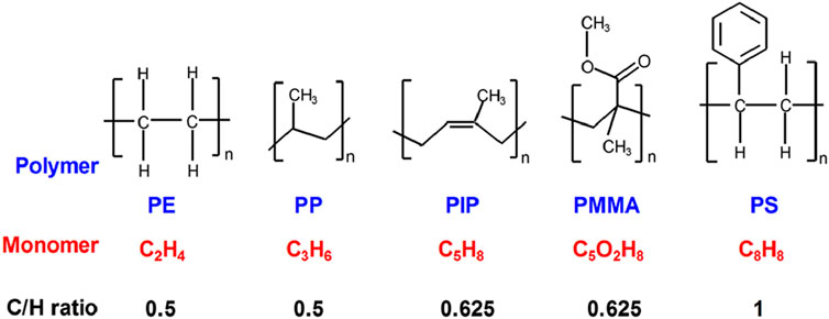
Figure 1. Chemical structures and C/H ratios of polyethylene (PE), polypropylene (PP), polyisoprene (PIP), poly (methyl methacrylate) (PMMA), and polystyrene (PS). This figure is reproduced from Nie (2017), with permission from John Wiley and Sons.

2.2 Time-of-flight secondary ion mass spectrometry (ToF-SIMS)

A ToF-SIMS IV instrument from ION-TOF (Münster, Germany), equipped with a liquid metal ion gun (LMIG), was used to collect negative secondary ion mass spectra on samples of PE, PP, PIP, PS and cross-linked PMMA generated by bombarding the surface using a pulsed 25 keV Bi₃⁺ primary ion beam at a fixed incident angle of 45° to the sample surface. The DC target current of the primary ion beam was measured at approximately 5 nA, reflecting the flux of ions generated by the liquid metal ion gun (LMIG) source and delivered to the target. For ToF-SIMS analysis, the primary ion beam was pulsed at 10 kHz, with each pulse maintained at a width of 1 ns. This pulsing mechanism achieved a target current of approximately 1 pA, which corresponds to 624 ions per pulse (commonly referred to as a “shot” in ToF-SIMS). This value was calculated based on the target current (1 pA), the elementary charge (1.602 × 10⁻¹⁹ C), and the pulse rate (10 kHz). The base pressure of the analytical chamber was on the order of 1 × 10⁻⁷ mbar.

The secondary ions were extracted by a 2-kV electric field between the sample and the extractor position perpendicular to the sample surface, imparting them with a kinetic energy of 2 keV (if singly charged). These ions then traversed a reflectron-type flight tube and ultimately reached a microchannel plate, generating a cascade of electrons. A scintillator converted these electrons into photons, which were amplified and measured by a photomultiplier tube. The detection system, comprising these three devices, effectively captured both the quantity of ions and their specific arrival times, denoted as t, as described by the following equation:

z q V = \frac{1}{2} m {(\frac{L}{t - t_{0}})}^{2}

where z represents the charge number, q is the elementary charge, V is the extraction voltage, m is the mass, L is the flight length, and t-t₀ is the flight time. The detection times of these ions were converted to mass-to-charge ratios (m/z) using ubiquitous hydrogen and hydrocarbon ions, as well as other known species when required. In practice, nearly all secondary ions detected in ToF-SIMS are singly charged (i.e., z = 1). The only exception observed by this author was calcium, which is typically detected as Ca⁺ at m/z 40 but may also appear as Ca²⁺ at m/z 20 when Ca⁺ is sufficiently abundant.

The secondary ion mass spectra were collected by rastering the primary ion beam at 128 × 128 (16,384) pixels over an area of 300 μm × 300 μm, with each pixel bombarded by one shot of the primary ion beam, followed by measurement of the secondary ions and subsequently the charge neutralization step using a low-energy electron beam. This process was done with a cycle time of 100 µs, rendering an m/z range up to 900 (Though not applicable for our experiment, measuring ions having m/z values larger than 900 requires increase the cycle time). This process was repeated 18 times, resulting in a primary ion dosage of 2 × 10¹¹ cm^-2, which was much lower than the static limit of 1 × 10¹³ cm^-2. (Fletcher et al., 2007b). The acquisition time for each spectrum was 30 s.

The spectrum was calibrated using H⁻, CH⁻ and C₄H⁻, which was sufficient for the hydrocarbon ions dealt with in this article. Generally, for higher mass ions, calibration using other known species and evaluation of assignment accuracy, calculated by (m/z value of the peak–m/z value of the assigned ion)/(m/z value of the assigned ion) and expressed by ppm, may be required. The mass resolution, calculated as the m/z value at the peak center divided by the full width half maximum of the peak, for C₂H⁻ and C₆H⁻ were 3400 and 4800, respectively. Multiple negative secondary ion mass spectra from each polymer collected and used for PCA. The measured ion intensities were corrected for the dead-time effect of the ion registration system using a Poisson correction. (Stephan et al., 1994). This adjustment is essential to account for the finite response time of the detection system, which can lead to an underestimation of ion counts at high signal rates. By applying this correction, the data more accurately reflects the true ion intensities, ensuring the reliability of subsequent analyses.

2.3 Principal component analysis (PCA)

The intensities of C_nH⁻ (n = 1–10) obtained on each of the four polymers (PE, PP, PIP and PS) were used for PCA. The data table is a m × n matrix, with m = M_total rows of measurements (ion intensities) and n = N_total columns of variables (C_nH⁻). (Nie, 2016). The total number of measurements (M_total) and the total number of variables (N_total) for one of the datasets in this study are 48 and 10, respectively. For simplicity and clarity, these values are used throughout the following description. A 48 × 10 data matrix X, with elements $x (m, C_{n} H)$ representing C_nH⁻ intensity in the m^th measurement, can be described as follows.

X = [\begin{array}{c} x (1, C_{1} H) & \dots & x (1, C_{10} H) \\ ⋮ & ⋱ & ⋮ \\ x (48, C_{1} H) & \dots & x (48, C_{10} H) \end{array}]

When the above matrix is standardized, each column is subtracted by its mean and divided by its standard deviation, resulting in each of the 10 columns having a unit variance $\sum_{m = 1}^{48} x {(m, C_{n} H)}^{2} / (48 - 1) = 1 .$ The prcomp() function (Prcomp, 2024) in R programing language (The R Project for Statistical Computing) was used to perform PCA not only on the ion intensity dataset normalized total ion intensity and the sum of all C_nH⁻ intensities, but also on the ion intensity datasets normalized by each C_nH⁻ intensity. In the latter case, there are only nine variables because the intensities of the normalizing C_nH⁻ column are all 1. Therefore, this column needs to be excluded because its variance is zero. The data matrices are standardized so that each variable has a unit variance, meaning that a 48 × 10 or a 48 × 9 data matrix has a total variance of 10 or 9, respectively.

The purpose of PCA is to project the original dataset onto a new set of coordinates, known as PCs. In this transformation, the first principal component, PC1, captures the largest variance in the original dataset. The second principal component, PC2, accounts for the largest variance of the remaining unexplained variance, and this process continues sequentially for subsequent components. The eigenvectors of X^TX, which is the covariance matrix (in our case it is the correlation matrix, as the dataset is standardized) of X, correspond to the PCs, while the eigenvalue of each eigenvector is the variance of each PC. Rather than dealing with the covariance (or correlation) matrix X^TX, singular value decomposition (SVD) of X provides the same results. Using the SVD approach, the prcomp(X) function in R utilizes the function svd(X) to return standard deviations ( $σ (P C_{k}),$ square root of variances) of PCs, PC scores and PC loadings, which are termed as sdev, x, and rotation, respectively.

Singular value decomposition of X is represented as X = USV^T, where U is the left singular matrix of size m × n, S is a diagonal matrix of size n × n containing the singular values in descending order, and V is the right singular matrix of size n × n, with V^T denoting the transpose of V. For a m × n data matrix (m = 48 measurements of variables C_nH⁻, with n = 1–10), if we denote singular values, scores and loadings of each PC (denoted as PC_k, with k = 1–10) as $d (P C_{k}), s (m, P C_{k}) \times d (P C_{k})$ and $l (P C_{k}, C_{n} H),$ respectively, then the three matrices associated with SVD of X can be expressed as follows.

U = [\begin{array}{c} s (1, P C_{1}) & \dots & s (1, P C_{10}) \\ ⋮ & ⋱ & ⋮ \\ s (48, P C_{1}) & \dots & s (48, P C_{10}) \end{array}]

S = [\begin{array}{c} d (P C_{1}) & \dots & 0 \\ ⋮ & ⋱ & ⋮ \\ 0 & \dots & d (P C_{10}) \end{array}]

V = [\begin{array}{c} l (C_{1} H, P C_{1}) & \dots & l (C_{1} H, P C_{10}) \\ ⋮ & ⋱ & ⋮ \\ l (C_{10} H, P C_{1}) & \dots & l (C_{10} H, P C_{10}) \end{array}]

The PC scores and loadings returned by x and rotation from prcomp() are US and V, respectively. Columns of US, i.e., $s (m, P C_{k}) \times d (P C_{k})$ present scores of all original measurements projected on ${P C}_{k}$ . Columns of V, $l (C_{n} H, P C_{k})$ , with n = 1 to 10, present loadings of all original variables on ${P C}_{k}$ , i.e., weights of every variable on transferring the original data points on ${P C}_{k}$ . All columns in U, V and V^T are orthogonal unit vectors. The columns in V correspond to the eigenvectors of correlation matrix of X^TX. With the singular values $d (P C_{k})$ divided by the square root of 48–1, the prcomp() function returns standard deviation, sdev, $σ (P C_{k})$ = $\frac{d (P C_{k})}{\sqrt{48 - 1}}$ for PCs from S, resulting in a diagonal matrix S′ containing ordered standard deviations $σ (P C_{k})$ , shown below.

S^{'} = [\begin{array}{c} σ (P C_{1}) & \dots & 0 \\ ⋮ & ⋱ & ⋮ \\ 0 & \dots & σ (P C_{10}) \end{array}]

What US = XV presents is that the original data points in X are projected on the new basis V, resulting in the transformed scores US. A score of a PC is shown in Equation 1, where the m^th measurements against all variables are $x (m, C_{n} H)$ , with n = 1 to 10 in our case for the 10 C_nH⁻. This set of 10 ion intensities are projected on a single $P C_{k}$ , as a single score, the m^th score $s (m, P C_{k}) \times d (P C_{k})$ .

s (m, P C_{k}) \times d (P C_{k}) = \sum_{n = 1}^{10} x (m, C_{n} H) \times l (C_{n} H, P C_{k}) (1)

On the other hand, the original data can be recovered from the scores US and loadings V via X = USV^T. For example, as shown in Equation 2, a single original C_nH⁻ intensity within the m^th measurement $x (m, C_{n} H)$ can be calculated from the m^th scores $s (m, P C_{k}) \times d (P C_{k})$ on all PCs (i.e., k = 1–10).

x (m, C_{n} H) = \sum_{k = 1}^{10} s (m, P C_{k}) \times d (P C_{k}) \times l (C_{n} H, P C_{k}) (2)

As shown in Equation 3, if we keep the first two (i.e., PC1 and PC2) and ignore the remaining PCs, then the original data is approximated as follows from their scores only on the first two PCs. However, how much the original datum is recovered depends on how good the loading vector of C_nH⁻, i.e., $l (C_{n} H, P C_{k})$ explains the scores $s (m, P C_{k}) \times d (P C_{k})$ corresponding to the original data $x (m, C_{n} H)$ .

x (m, C_{n} H) ≅ \sum_{k = 1}^{2} s (m, P C_{k}) \times d (P C_{k}) \times l (C_{n} H, P C_{k}) (3)

Therefore, as illustrated in Equations 1 and 2, PCA does not alter the original data; instead, it views the data to uncover underlying patterns or structures by focusing on their variability. The purpose of PCA is to visualize multivariate data, via dimensionality reduction, in 2D or 3D formats for easier interpretation and analysis. This is realized when dealing with the first two (as shown in Equation 3) or three PCs. We can thus visualize measurement scores and variable loadings of PC1 and PC2 as a score plot and a loading plot, respectively, which, when overlapped, form a biplot (Gabriel, 1971; Greenacre, 2010). The loading of a variable plotted in a biplot may be called the loading vector of the variable and expressed as an arrowed line from the origin of PC1 and PC2 axes to its PC1 and PC2 loadings. The biplot not only presents both the scores and loading vectors of the selected PCs, but also allows for the exploration of additional information correlating the scores, loadings, and the original data, as detailed below.

We follow the ggbiplot() (VQV, 2024) function from the ggplot2 package in R to display the scores of the 48 measurements as points and the loadings of the 10 (data normalized by total ion intensity or sum of the 10 C_nH⁻) or nine variables (data normalized by a C_nH⁻ intensity) as arrowed lines, both on the plane defined by PC1 and PC2. This function provides a correlation circle, within which all loading vectors are plotted. If a loading vector of a variable is close to the correlation circle, the variable is well explained by the two PCs. Conversely, if a loading vector is far away from the correlation circle, the variable is not explained well by the two PCs, indicating that it must be explained by other PCs.

In PCA biplots, the type that does not incorporate standard deviations into the loading vectors is referred to as the correlation biplot. In a correlation biplot, the focus is on representing the relationships between variables, which is particularly useful when the variables are on different scales or when the emphasis is on interpreting the relative contributions of variables to the PCs. In our analysis, standardization ensures that each variable contributes equally to the PCA by scaling their variances to 1. By multiplying the PC loadings, $l (C_{n} H, P C_{k})$ , by the standard deviation of the corresponding PC, $σ (P C_{k})$ , the resulting loading vector, $l (C_{n} H, P C_{k}) \times σ (P C_{k})$ , incorporates the variance explained by the PC. This scaling transforms the biplot into a covariance biplot, which reflects the absolute contributions of the variables to the variance in the dataset.

In the covariance biplot generated by ggbiplot(), the radius of the correlation circle, which is one for a standardized dataset, and the standard-deviation-incorporated loading vectors are further scaled (VQV, 2024) by multiplying a fact (e.g., 1.5) to align with the scaled scores, which is achieved by dividing $(m, P C_{k}) \times d (P C_{k})$ with $σ (P C_{k})$ . This additional scaling facilitates a more balanced visualization of the variable vectors and measurement scores. Without this adjustment, the scores are often positioned too far from the loading vectors, making the biplot less interpretable. This refinement enhances the clarity of the relationships between variables and samples in the PCA results. The ggbiplot() function also offers data ellipses for the scores associated with each of the four polymers, providing a clear and effective visual representation of the grouped scores and their distribution in the biplot. The scores of each sample are plotted with a 68% confidence level ellipse, representing one standard deviation around the mean, assuming the data are approximately normally distributed.

Specifically, scores from US and loading vectors from VS′ for the first two PCs are plotted. In this context, the projection of a pair of scores [e.g., $s (m, P C 1) and s (m, P C 2)$ ] from US onto the loading vector of a variable C_nH⁻ [ $l (C_{n} H, P C_{1}) and l (C_{n} H, P C_{2})$ ] from V approximates the ion intensity of that variable (in the original dataset) $x (m, C_{n} H)$ , as shown below.

x (m, C_{n} H) ≅ \frac{\sum_{k = 1}^{2} s (m, P C_{k}) \times d (P C_{k}) \times l (C_{n} H, P C_{k})}{\sqrt{\sum_{k = 1}^{2} {[l (C_{n} H, P C_{k}) \times σ (P C_{k})]}^{2}}} (4)

The cosine of the angle (or the correlation) between the loading vectors of two variables C_xH⁻ and C_yH⁻ from VS′ approximates their correlation in the original dataset, as shown below.

\frac{1}{47} \sum_{m = 1}^{48} x (m, C_{x} H) \times x (m, C_{y} H) ≅ \sum_{k = 1}^{2} l (C_{x} H, P C_{k}) \times σ (P C_{k}) \times l (C_{y} H, P C_{k}) \times σ (P C_{k}) (5)

The PCA results (i.e., sdev, x, and rotation) were saved from prcomp() and ellipses data of each polymer were obtained using the ellipse (Ellipse, 2024) package. These data are used to plot covariance biplots, using Microsoft Excel, in this article for the first two PCs. The scores are divided and the loading vectors multiplied by the standard deviation, respectively. These biplots offer comprehensive insights, including measurement scores, variable loadings, relationships between scores and loadings, as well as the underlying implications (Equation 4) and correlations (Equation 5) within the original data.

3 Results and discussion

Table 1 presents the normalized intensities of negative hydrocarbon ions, specifically C_nH⁻ (where n ranges from 1 to 10), calculated as a ratio to the total ion intensity for each measurement. This normalization ensures that the data are comparable across samples, reducing variability due to instrumental or experimental conditions. The normalized intensities will be standardized using the prcomp() function in R for PCA, a multivariate statistical technique employed to uncover patterns and relationships within the dataset. PCA reduces the dimensionality of the data while preserving the most significant variance, enabling the differentiation of polymer samples based on the variability of the C_nH⁻ ions.

Table 1

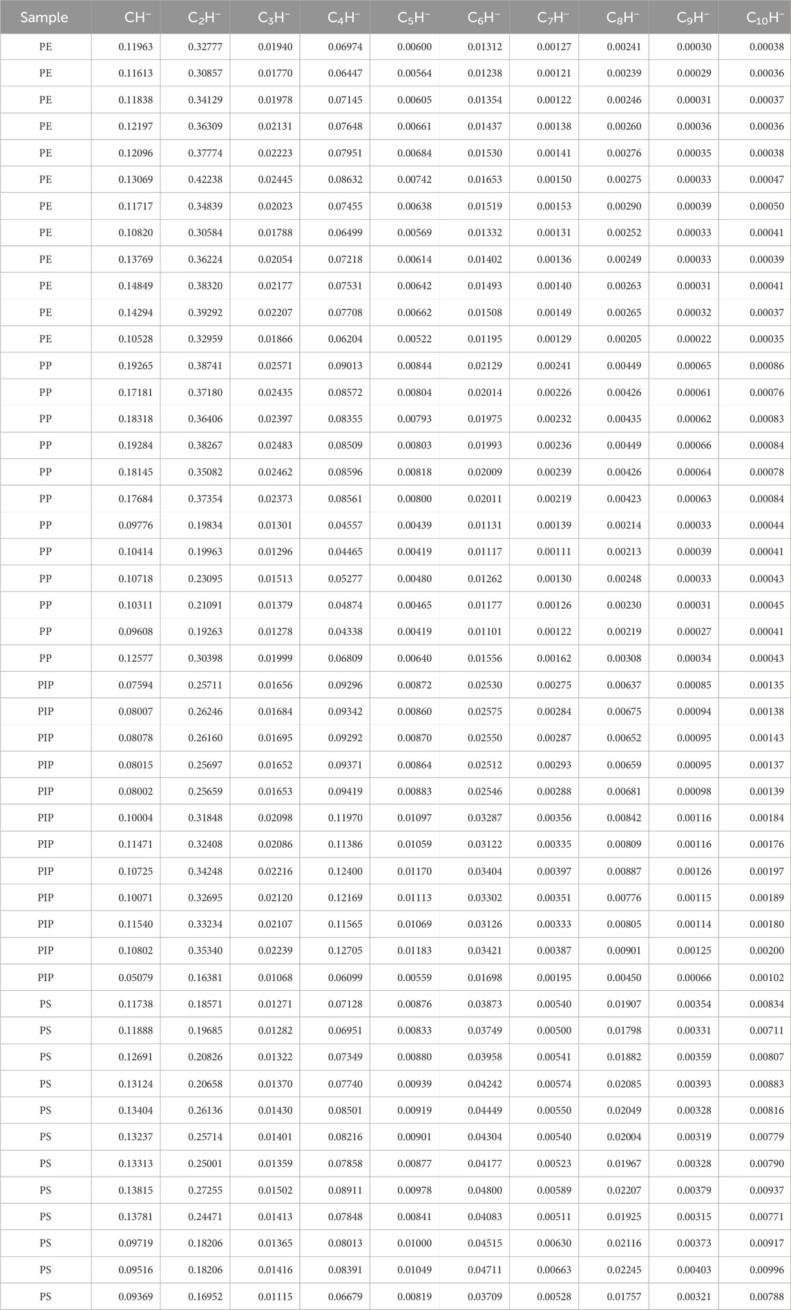
Table 1. Intensity data of C_nH⁻ ions, normalized to the total ion intensity, for 12 measurements each of polyethylene (PE), polypropylene (PP), polyisoprene (PIP), and polystyrene (PS). Data for 39 out of the 48 measurements are reproduced from Table 1 in Nie (2017), with permission from John Wiley and Sons.

Table 2 shows the variances of PC1, PC2, and PC3, as well as the explained percentage of variance of PC1 and cumulative explained variance for PC two and PC3, determined by the PCA of 12 datasets with ion intensities in each measurement normalized to their total ion intensity (Table 1), the intensities of each C_nH⁻, and the sum of the intensities of the 10 C_nH⁻. The lowest cumulative variance explained by the first two and three PCs is 87.3% and 98.4%, respectively, which is the case for the dataset normalized by the total ion intensity for each of the 48 measurements. Other normalizations resulted in higher cumulative percentages for the first two and three PCs.

Table 2

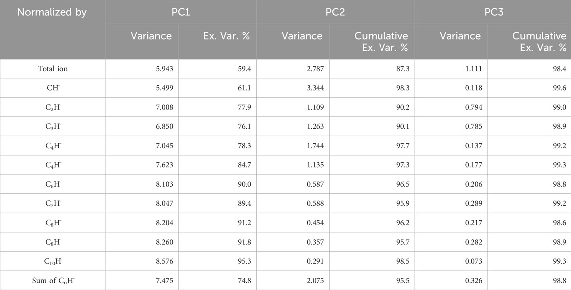
Table 2. Variance of PC1 to PC3, along with the percentage of explained variance for PC1 and the cumulative explained variance for PC2 and PC3, calculated for each of the 12 datasets normalized by (1) the total ion intensity, (2) the intensity of individual C_nH¯ ions, and (3) the sum of the intensities of the 10 C_nH⁻ ions. The ion intensity data were obtained from measurements on polyethylene (PE), polypropylene (PP), polyisoprene (PIP), and polystyrene (PS).

Because the first two PCs explained the vast majority of the variance across all datasets, we present the PCA results only for PC1 and PC2. However, we emphasize that, in principle, this decision is provisional and contingent on the confirmation of sufficient cumulative variance explained by these components. In our analysis, the high cumulative variance—ranging from 87.3% to over 98.5% for the first two PCs—justifies the sufficiency of retaining only PC1 and PC2 for our specific datasets. Furthermore, we examined the higher PCs but found no significant contributions from them. This approach ensures that our methodology is data-driven and adaptable to different contexts.

Figure 2A shows scaled covariance biplot for the PCA results for the ion intensity dataset normalized by total ion intensity (Table 1), which is further standardized before PCA. We also normalized the dataset by each of the 10 C_nH⁻ ion intensities, generating PCA results shown in Figures 2B–F, 3A–E for n = 1 to 10, respectively. Finally, Figure 3F presents the covariance biplot for PCA results of the ion intensity dataset normalized by the sum of the 10 C_nH⁻ intensities. The PCA results in Figures 2, 3 are visualized in biplots plotted using results of the first two PC measurement scores, variable loadings and standard deviations calculated via prcomp() in R, displaying overlapped plots of scores (points) divided and loadings (arrowed lines) multiplied by standard deviation, respectively. The scaling applied to the scores, loading vectors, and the correlation circle ensures a more balanced and interpretable visualization of the PCA results, as elaborated in the methods section.

Figure 2

Figure 2. Principal component analysis (PCA) results, with 68% confidence level ellipses, for polyethylene (PE), polypropylene (PP), polyisoprene (PIP), and polystyrene (PS), displayed as scaled covariance biplots (i.e., with the PCA scores divided by their standard deviation and the loading vectors multiplied by their standard deviation). The analysis is based on six ion intensity datasets normalized by total ion intensity (A) and by C_nH⁻ intensity with n = 1 (B), 2 (C), 3 (D), 4 (E) and 5 (F), respectively. The variances explained by the first two principal components (PCs) for the datasets are indicated in the labels for PC1 (x-axis) and PC2 (y-axis). The correlation circle and loading vectors are scaled up by a factor of 1.5 for a more balanced and visually interpretable biplot. The normalizing C_nH⁻ ion is excluded from each dataset, as all its measurements for the four polymers are normalized to 1. The scores of PC1 and PC2 for the four polymers are represented as points, while the loading vectors (arrowed lines) of C_nH⁻ ions are labeled by their respective n for clarity. The results shown in (A, E) are reproduced from Figure 5 and Figure 7, respectively, Nie (2017), with permission from John Wiley and Sons.

Figure 3

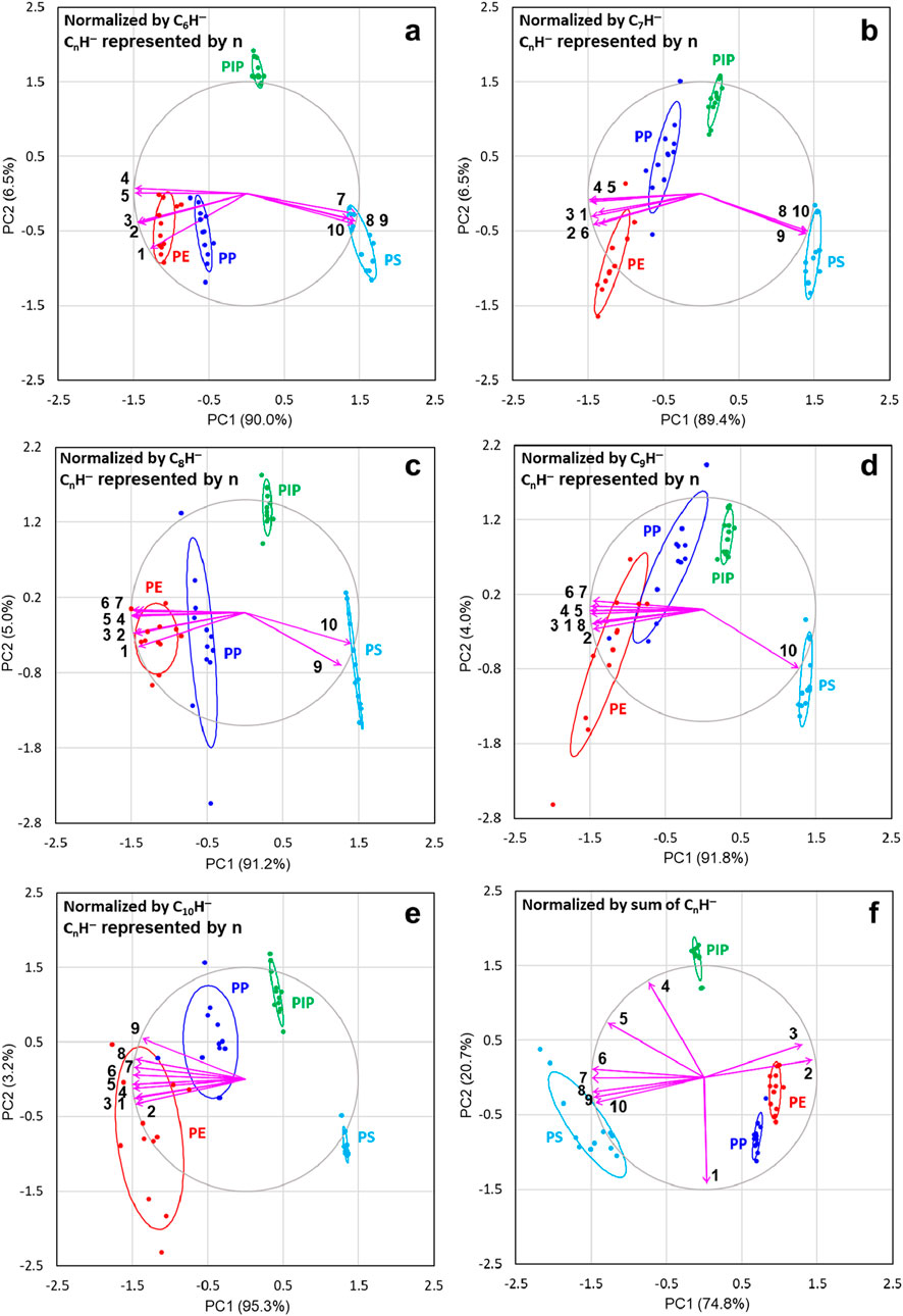
Figure 3. Principal component analysis (PCA) results, with 68% confidence level ellipses, for polyethylene (PE), polypropylene (PP), polyisoprene (PIP), and polystyrene (PS), displayed as scaled covariance biplots (i.e., with the PCA scores divided by their standard deviation and the loading vectors multiplied by their standard deviation). The analysis is based on six ion intensity datasets normalized by C_nH⁻ intensity with n = 6 (A), 7 (B), 8 (C), 9 (D) and 10 (E), respectively, as well as by the sum of the intensities of the 10 C_nH⁻ ions (F), with n = 1 to 10. The variances explained by the first two principal components (PCs) for the datasets are indicated in the labels for PC1 (x-axis) and PC2 (y-axis). The correlation circle and loading vectors are scaled up by a factor of 1.5 for a more balanced and visually interpretable biplot. The normalizing C_nH⁻ ion is excluded from each dataset, as all its measurements for the four polymers are normalized to 1. The scores of PC1 and PC2 for the four polymers are represented as points, while the loading vectors (arrowed lines) of C_nH⁻ ions are labeled by their respective n for clarity.

As shown in Figure 2A, the first two PCs explain 87.3% of the total variance of the original ion intensities normalized by total ion intensity, where the total variance is 10 (contributed by the 10 variables each with unit variance). Therefore, PCA leads to dimensionality reduction, that is, the two new variables (PCs) can describe the total variance of 10 of the original datasets with only 12.7% of the total variance unexplained. The first two PCs for CH⁻ (Figure 2B), C₂H⁻ (Figure 2C), C₃H⁻ (Figure 2D), C₄H⁻ (Figure 2E) and C₅H⁻ (Figure 2F) normalization explain 98.3%, 90.2%, 90.1%, 97.7% and 97.3% of the total variance, respectively. As shown in Figures 3A–E, the first two PCs for datasets normalized by the remaining C_nH⁻ explain more than 95% of the total variance. Figure 3F demonstrates that normalization by the sum of the C_nH⁻ is effective, as the scores for each polymer cluster are well separated from each other and the first two PCs explain 95.5% of the total variance.

Therefore, PCA allows the visualization of the relationships between measurements and between variables, as well as between these two groups in the first two PCs. For example, as shown in Figure 2A, the scores for the four polymers are clustered, with rather large variations for PE, PP and PIP on PC2. Clearly, PCA can differentiate the polymers via the variability in their ion intensities. This is a useful analytical approach because the ion mass spectra of these polymers are quite similar. More precisely, there are no unique ions to any of the four polymers. In this situation, one relies on the variability of ions, rather than their identities, to differentiate the polymers.

A biplot is also capable of visualizing correlations between variables and contributions of variables to scores. If the angle between the loading vectors of two variables is close to 0°, 180° or 90°, then the two variables are positively correlated, negatively correlated or uncorrelated, respectively. As shown in Figure 1A, C₆H⁻ to C₁₀H⁻ are highly correlated because angles between their loading vectors are small. For example, the angle between the loading vectors of C₆H⁻ and C₇H⁻, shown in Figure 2A, is 8.24°, as estimated from the correlation of 0.989478808. This value is derived from the correlation between the loading vectors on PC1 and PC2, with the standard deviations $σ (P C_{1})$ and $σ (P C_{2})$ incorporated in V, as shown on the right-hand side of Equation 5. This is very close to the correlation of 0.986733778 (corresponding to an angle of 9.24°) between C₆H⁻ and C₇H⁻ in the original dataset, calculated using the left-hand side of Equation 5. The loading plot is crucial for visualizing relationships, more precisely, the correlations, among all variables.

As shown in Figure 2A, the contributions of C₆H⁻ to C₁₀H⁻ to the scores of PS are significant, as their loading vectors point towards these scores. C₂H⁻ and C₃H⁻ are positively correlated as their loading vectors overlap. These two ions contribute to the scores of PP and PE. The loading vectors of CH⁻ and C₅H⁻ are less relevant to other ions. The loading vector of C₄H⁻ is approximately in the middle between those of the two groups of ions (i.e., C₆H⁻ to C₁₀H⁻ vs C₂H⁻ and C₃H⁻), indicating that it is not heavily correlated to either group.

As previously reported, our PCA results clarified that polymers with larger and smaller carbon densities favor the generation of larger and smaller C_nH⁻ ions, respectively (Nie, 2016; Nie, 2017). As a medium C_nH⁻ ion, C₄H⁻ contributes more than other C_nH⁻ ions to scores of PIP, which is the polymer with a medium carbon density. These experimental measurements are the underlying mechanism for success in using C₄H⁻ as the reference ion to access carbon densities of polymers and cross-linking degrees of PMMA (Naderi-Gohar et al., 2017).

From the covariance biplot, one can roughly estimate each original datum $x (m, C_{n} H)$ from the projection of a corresponding score determined by $s (m, P C_{1})$ and $s (m, P C_{2})$ onto the loading vector of a variable C_nH⁻. For example, for the results shown in Figure 2A, the projection of a score at $s (48, P C_{1}) = - 3.470661351$ and $s (48, P C_{2}) = 1.8242691$ onto the loading vector defined by $l (C_{10} H, P C_{1}) \times σ (P C_{1}) = - 0.963385438$ and $l (C_{10} H, P C_{2}) \times σ (P C_{2}) = 0.061623353$ is $1.490513115$ , as calculated using Equation 4, which closely approximates the original datum $x (48, C_{10} H) = 1.540468817$ , which corresponds to the standardized value of the C₁₀H⁻ intensity from the PS measurement listed at the bottom of Table 1 (i.e., 0.00788).

Figure 2B shows the biplot for the dataset normalized by CH⁻. Compared to Figure 2A, scores and loading vectors rotate roughly 180°, which is not important since only the clustering of scores and their relationship with the loading vectors provide useful information. The most notable change is a significant reduction in scattering of PC2 scores for PP and PIP. The loading vector of C₄H⁻ explains the scores of PIP extremely well. Loading vectors of C₂H⁻ and C₃H⁻ are slightly further away from the scores of PE and PP. The major contributors to scores of PS are C₈H⁻ to C₁₀H⁻.

As shown in Figure 2C, when normalized by C₂H⁻, the scores of PS become more scattered. The most contributing ion to the scores of PIP is now C₃H⁻. The contributing ions to the scores of PS are C₆H⁻ to C₁₀H⁻. Although the loading vector of CH⁻ overlaps with that of C₁₀H⁻, it is not considered a contributor to the scores of PS because it is short (i.e., far away from the correlation circle), suggesting that this variable is not well explained by PC1 and PC2.

For the C₃H⁻ normalization case shown in Figure 2D, C₆H⁻ to C₁₀H⁻ contribute the most to scores of PS, with C₁H⁻, C₄H⁻ and C₅H⁻ making considerable contributions as well. On the other hand, there are no loading vectors pointing to the PE, PP and PIP. Like what is shown in Figure 2C, the scores of PS spread on PC2. Therefore, from Figures 2B–D, it is evident that using smaller ions CH⁻ to C₃H⁻ to normalize the ion intensity dataset removes contributing ions to the scores of the two lower carbon density polymers, PE and PP. Additionally, there are no contributing ions to the scores of the medium carbon density polymer PIP when C₃H⁻ is used for normalization.

As shown in Figure 2E, when C₄H⁻ is used for normalization, the relationships between loading vectors change significantly compared to those shown in Figures 2B–D. Another observation from the PCA results in Figure 2E is that the scatter in scores for PP and PIP is significantly reduced compared to their counterparts normalized to total ion intensity, as shown in Figure 2A. As shown in Figures 2F, 3A–E, the loading vectors of C₅H⁻ to C₁₀H⁻ almost overlap and point to the scores of PS, while the overlapped loading vectors of C₂H⁻ and C₃H⁻ point to the scores of PE and PP. These results are quite similar to those in Figure 2A, where C₆H⁻ to C₁₀H⁻ are contributing ions to the scores of PS. However, with normalization using C₄H⁻, C₅H⁻ is more relevant to the scores of PS than when the ion intensity dataset is normalized by total ion intensity. Similar to Figure 2A, C₂H⁻ and C₃H⁻ are the two contributing ions to the scores of PE and PP.

It is worth mentioning that the angles between the loading vector of CH⁻ and those of C₆H⁻ to C₁₀H⁻ in both Figures 2A, E are close to 90°, indicating that CH⁻ is not correlated with these larger C_nH⁻ ions. There are no loading vectors pointing to the PIP scores in Figure 2E, as the contributing ion, C₄H⁻, is used to normalize the dataset and therefore no longer contributes to the variance in the newly normalized dataset. As discussed above and elsewhere, (Nie, 2017), normalization using C₄H⁻ serves to classify contributing ions more elegantly and remove information irrelevant to the chemical structures, resulting in less scattered scores for most of the polymers.

Figure 2F shows that when C₅H⁻ is used for normalization, the loading vector of C₄H⁻ turns towards the scores of PE and PP. This suggests that C₄H⁻ contributes more to the scores of PE and PP than in any of the cases normalized by a C_nH⁻ ion smaller than C₄H⁻. The loading vectors of the rest of C_nH⁻ (excluding C₅H⁻) ions are similar to those in the C₄H⁻ normalization case.

As shown in Figures 3A–E, using a C_nH⁻ ion (n = 6–10) to normalize the ion intensity dataset causes the loading vectors of all ions smaller than the normalizing ion C_nH⁻ to turn towards the scores of PE and PP. When C₁₀H⁻ is used for normalization, as shown in Figure 3E, all ions contribute to PE and PP. We observed that when larger C_nH⁻ ions are used for normalization, the scores of lower carbon density polymers, i.e., PE and PP, become more scattered, as shown in Figures 3D, E. Finally, Figure 3F presents the biplot for the dataset normalized by the sum of the 10 C_nH⁻ ions. This normalization effectively separates the scores of the four polymers and clearly illustrates the contributions of the C_nH⁻ ions to the scores, which are largely similar to those observed in the dataset normalized by total ion intensity (Figure 2A). An additional advantage of this normalization by the sum of the 10 C_nH⁻ intensities, compared to normalization by total ion intensity, is the significantly reduced scatter in the scores of PE, PP, and PIP.

By comparing all PCA results in Figures 2, 3 for the 12 datasets normalized by the total ion intensity, the intensities of C_nH⁻ with n = 1 to 10 and the sum of the intensities of the 10 ions, it becomes clear that C₄H⁻ is the best reference ion. This is because it maintains the correlations between ions almost the same as when normalization is done using total ion intensity, while removing variability irrelevant to the chemical structures of the polymers. It is evident in Figures 2, 3 that normalization with other C_nH⁻ significantly changes the correlation of some ions. This highlights that certain ions are better than others in revealing the chemical structures of the materials under investigation. Our PCA results exemplify how PCA provides clues to uncover more useful chemical structures or information hidden in the data.

Another observation from the PCA results, where ion intensities were normalized by various C_nH⁻ ions, is that the PC1 scores exhibit a consistent trend across the four polymers, irrespective of the specific C_nH⁻ ion used for normalization. This consistency is clearly illustrated in Figures 2B–F, 3A–E. Specifically, the scores of PE, PP, PIP, and PS align with increasing carbon density. As shown in Figures 2A, 3F, this trend is also true in the case where the total ion intensity and the sum of the 10 C_nH⁻ intensities are used for normalization, respectively. It is thus clear that the PC1 scores of the ion intensity data of the four polymers, regardless of how the intensities of the C_nH⁻ ions are normalized, capture the variability dictated by the carbon density of the polymers. This may lead to correlation between PC1 scores and ρ, the intensity ratio between C₆H⁻ and C₄H⁻, which has been proved to be a measure of the carbon density of polymers. (Nie, 2016; Nie, 2017).

To examine the relationship between PC1 scores and ρ, as well as between PC2 scores and ρ, we plot in Figure 4 the PC1 and PC2 scores for the 10 ion intensity datasets, normalized by each of the ten C_nH⁻ (n = 1–10) ions, as a function of ρ. As can be determined from the intensities of C₆H⁻ and C₄H⁻ in Table 1, the values of ρ are 19.4% ± 0.6%, 23.9% ± 0.8%, 27.3% ± 0.3%, and 54.1% ± 1.5% for PE, PP, PIP, and PS, respectively. Each PCA score point obtained for each intensity dataset is an average over the scores of a polymer, with both the standard deviations of the scores and ρ plotted. The four points for the four polymers in each dataset are connected by a line for clarity.

Figure 4

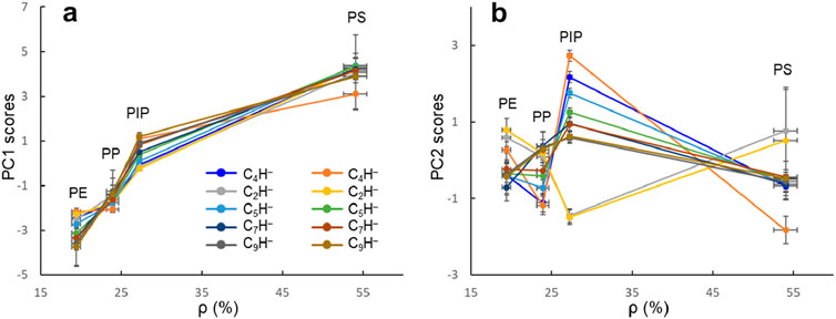
Figure 4. PC1 (A) and PC2 (B) scores as a function of ρ (the intensity ratio between C₆H⁻ and C₄H⁻) for polyethylene (PE), polypropylene (PP), polyisoprene (PIP), and polystyrene (PS). The ten datasets are each normalized by a C_nH⁻ (n = 1–10) as indicated in (A).

As shown in Figure 4A, although the PC one scores for the four polymers vary depending on the normalizing ion, the trend that PC1 scores increase with ρ is evident. We discovered that PC1 scores and ρ are related, regardless of the ion used normalize the intensity dataset. This observation confirms that both ρ and PC1 scores reflect carbon density of the polymers. Notably, for polymers lacking unique ions in their negative ion mass spectra, this data-driven analytical approach is effective and can quantitatively differentiate the polymers.

Principal component analysis provides opportunities to reveal underlying structures in the data. This is advantageous because data collected may not explicitly reflect the information one seeks. In the case demonstrated in this article, the secondary ion mass spectra provide information on ions and their intensities measured from polymers, rather than anything explicitly pointing to their carbon density. While ρ is a measure of carbon density (Nie, 2016) of polymers, PC1 scores appear to capture the trend of carbon density of the polymers. In other words, without PCA, one may not be able to realize the connection between the carbon density (the structural property of polymers) and the variability of the C_nH⁻ intensities collected using ToF-SIMS.

Polymers, especially polymeric coatings, are commonly cross-linked to meet requirements on mechanical strength and thermal stability. (Chen et al., 2020; Mayumi et al., 2021; Ceylan et al., 2023; Li and Gau, 2020). Cross-linking can be viewed as a process involving hydrogen loss, leading to increased carbon densities. Therefore, the ToF-SIMS approach for gauging carbon density in polymers should be applicable for assessing the degree of cross-linking of polymers. We compared cross-linked PMMA with PE, PP, PIP, and PS to validate the criterion of ρ correlated with the cross-linking degrees of PMMA. Table 3 presents the C_nH⁻ intensities normalized by the total ion intensity for each of the 48 measurement for the PMMA samples. As calculated from the ion intensities of C₆H⁻ and C₄H⁻ in Table 3, ρ for the control is 32.2% ± 1.0%. The values of ρ for cross-linked PMMA films treated with HHIC for 0, 100, and 500 s increase to 44.7% ± 1.1%, 55.1% ± 1.1%, and 64.7% ± 2.2%, respectively.

Table 3

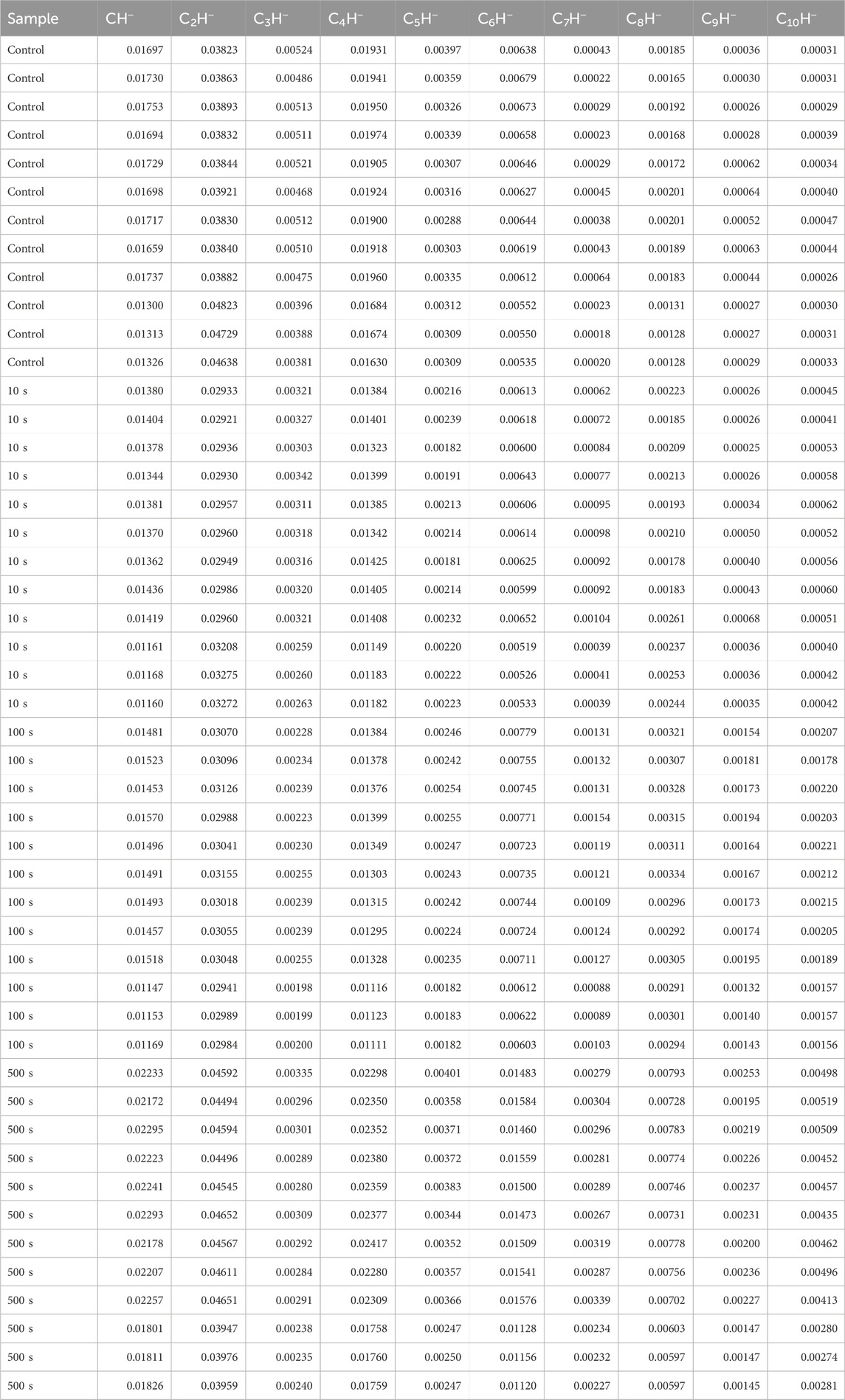
Table 3. Intensity data of C_nH⁻ ions, normalized to the total ion intensity, for a pristine poly (methyl methacrylate) (PMMA) film (control) coated on a Si wafer, and PMMA films subjected to HHIC treatment for 10, 100, and 500 s to induce cross-linking.

Principal component analysis is conducted by combining the ion intensity dataset for PMMA in Table 3 and the ion intensity dataset for PE, PP, PIP, and PS in Table 1. Figure 5 shows the biplot of the PCA results of C_nH⁻ normalized by C₄H⁻ for PE, PS, PIP and PS, as well as the pristine (control) and cross-linked PMMA films obtained by HHIC treatments for different periods. Together, PC1 and PC2 explain 87.3% of the total variance. The clustering of the four polymers largely remains the same as shown in Figure 2E, regardless of the addition of the PMMA data to the dataset for PCA. As indicated by the inserted box in Figure 5, the clustering of the scores of the pristine PMMA and cross-linked PMMA align with direction indicating the increase of carbon density, as defined by the clustering of the scores of PE, PS, PIP and PS. For the heavily cross-linked PMMA films treated with HHIC (Trebicky et al., 2014) for 100 and 500 s, the contributing ions are C₆H⁻ to C₁₀H⁻. The correlation of the scores on PC1 with the carbon densities of the polymers and the cross-linked PMMA films is evident. This provides a new approach to assessing the cross-linking degree of polymers, which is an important advancement for extremely thin polymer films, where conventional techniques (Hirschl et al., 2013; Bergmann et al., 2023) to characterize their cross-linking degrees are difficult or impossible.

Figure 5

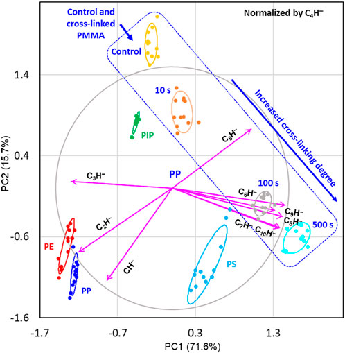
Figure 5. Principal component analysis (PCA) results, with 68% confidence level ellipses, for polyethylene (PE), polypropylene (PP), polyisoprene (PIP), and polystyrene (PS), as well as pristine (control) and cross-linked poly (methyl methacrylate) (PMMA), displayed as scaled covariance biplots (i.e., with the PCA scores divided by their standard deviation and the loading vectors multiplied by their standard deviation). The cross-linked PMMA films were obtained by hyperthermal hydrogen bombardment for 10, 100 and 500 s. The ion intensities of the nine C_nH⁻ ions (n = 1 to 3 and 5–10) are normalized by the intensity of the C₄H⁻ ion. The variances explained by the first two principal components (PCs) for the dataset are indicated in the labels for PC1 (x-axis) and PC2 (y-axis). The correlation circle and loading vectors are scaled up by a factor of 1.5 for a more balanced and visually interpretable biplot. The normalizing C₄H⁻ ion is excluded from the dataset, as all its measurements for the four polymers are normalized to 1. The scores of PC1 and PC2 for the samples are represented as points, while the loading vectors (arrowed lines) are labeled by C_nH⁻. The scores of the PMMA samples are indicated by the inserted box.

Therefore, our ToF-SIMS approach offers a novel method for examining the cross-linking degree of the surface of polymer coatings. Giving the versatile applications of PMMA, both as a coating material (Naderi-Gohar et al., 2017; Trebicky et al., 2014) and as a matrix (Ceylan et al., 2023; Li and Gau, 2020; Hosseinioun et al., 2019; Liu et al., 2023) for polymer composites, ToF-SIMS emerges as a highly versatile analytical technique. It not only enables probing surface chemistry of the polymer, but also serves as a chemically selective technique for elucidating their chemical characteristics, particularly in terms of carbon density.

To evaluate the robustness of ρ as a measure of carbon densities in polymers and the reproducibility of the PCA approach for classifying polymers based on their negative ions (C_nH⁻) detected by ToF-SIMS, we conducted additional experiments. These included ToF-SIMS measurements on multiple particles of PP, multiple pellets of PP and PS, a thick paste of PIP on aluminum foil, and a film of a PP-PS mixture (2:3 by weight) prepared from their xylene solution on aluminum foil. These experiments were designed to verify the consistency of differentiating polymers using their carbon densities, as evaluated by ρ, and their clustering in PC1 and PC2 scores. Additionally, the PP-PS mixture was used to assess whether it could reflect the averaged contributions of its component polymers. Table 4 presents the C_nH⁻ intensities, normalized by the total ion intensity, for each of the 48 measurements of the four polymers, along with 12 measurements of the PP-PS mixture.

Table 4

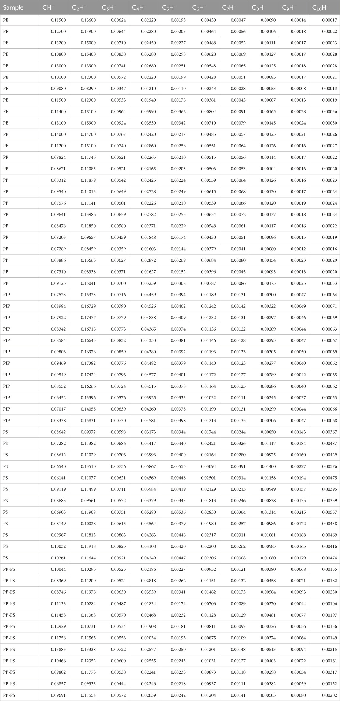
Table 4. Intensity data of C_nH⁻ ions from a new experiment, normalized to the total ion intensity, for 12 measurements each of polyethylene (PE), polypropylene (PP), polyisoprene (PIP), polystyrene (PS), and a PP-PS mixture.

Figure 6A illustrates ρ, the ion intensity ratio between C₆H⁻ and C₄H⁻, derived from Tables 1, 4 for two sets of experiments conducted approximately 10 years apart. The ρ values for PE, PP, PIP, and PS from both experiments exhibit striking consistency: 19.4% ± 0.6% vs 19.8% ± 0.5% for PE, 23.9% ± 0.8% vs 23.4% ± 0.6% for PP, 27.3% ± 0.3% vs 26.4% ± 0.9% for PIP, and 54.1% ± 1.5% vs 54.2% ± 0.8% for PS. The close agreement between the ρ values from these independent experiments—despite differences in the sources of PP (a commercial film vs pure pellet) and PS (a commercial cup vs pure pellet)—highlights the robustness of ρ as a reliable metric for estimating the carbon densities of polymers. This consistency further reinforces the utility of ρ in characterizing polymer structures across varying experimental conditions and extended timeframes, demonstrating its applicability as a stable and reproducible analytical tool.

Figure 6

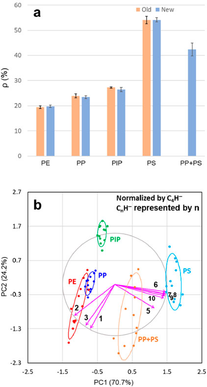
Figure 6. Comparison of ion intensity ratio between C₆H⁻ and C₄H⁻, denoted as ρ, between the old and new experiments (A). Shown in (B) are new-experiment principal component analysis (PCA) results, with 68% confidence level ellipses, for polyethylene (PE), polypropylene (PP), polyisoprene (PIP), and polystyrene (PS), as well as a PP-PS mixture, displayed as scaled covariance biplots (i.e., with the PCA scores divided by their standard deviation and the loading vectors multiplied by their standard deviation). The ion intensities of the nine C_nH⁻ ions (n = 1 to 3 and 5–10) are normalized by the intensity of the C₄H⁻ ion. The variances explained by the first two principal components (PCs) for the dataset are indicated in the labels for PC1 (x-axis) and PC2 (y-axis). The correlation circle and loading vectors are scaled up by a factor of 1.5 for a more balanced and visually interpretable biplot. The normalizing C₄H⁻ ion is excluded from the dataset, as all its measurements for the four polymers are normalized to 1. The scores of PC1 and PC2 for the samples are represented as points, while the loading vectors (arrowed lines) of CnH¯ ions are labeled by their respective n for clarity.

Additionally, as shown in Figure 6A, the PP-PS mixture exhibits a ρ value of 42.4% ± 2.6%, which closely aligns with the calculated value of 41.9%. This calculated value is derived from the measured ρ values of PP (23.4%) and PS (54.2%) and their weight ratio (2:3). The agreement between the experimental and calculated ρ values highlights the applicability of the ρ approach for estimating the carbon densities of polymer mixtures. This finding underscores the versatility of ρ as a reliable metric, not only for individual polymers but also for complex systems such as polymer blends, further validating its utility in characterizing carbon densities across a range of material compositions.

The primary limitation in estimating ρ stems from potential interferences with the C₆H⁻ intensity, which can be influenced by the presence of species with overlapping or closely matching m/z values. For example, ions such as C₃H₂OF⁻, SiC₂H₅O⁻, C₂H₃NO₂¯, and C₃H₅O₂¯ can inflate the measured C₆H⁻ intensity, thereby introducing uncertainties in the determination of ρ. Of course, this and any other interferences affecting the intensities of C_nH⁻ ions will lead to their overestimation, ultimately compromising the accuracy and reliability of the PCA results.

The PCA results of the new experiment dataset, normalized by the C₄H⁻ intensity, are presented in Figure 6B as a scaled covariance biplot for PE, PP, PIP, PS, and the PP-PS mixture. The five samples are well-separated in the PC1 and PC2 landscape, demonstrating clear differentiation among the polymers. Notably, the scores of the PP-PS mixture are positioned between those of PP and PS, reflecting the averaging effect of the two component polymers in their PCA results. This observation highlights how the mixture’s properties are intermediate to its individual constituents.

When compared to the PCA results for the old dataset shown in Figure 2E, the PCA results for new dataset in Figure 6B exhibits a roughly similar pattern. However, unlike ρ, which provides a quantitative measure of carbon densities in polymers, PCA scores primarily reveal trends related to ρ rather than offering direct quantification. The primary role of PCA is to separate polymers based on their distinct variabilities in the intensities of C_nH⁻ ions. This PCA-enabled ToF-SIMS analytical approach demonstrates high effectiveness in the PC1 and PC2 landscape for differentiating polymers and, potentially, their mixtures. The utility of the PCA approach lies in capturing the inherent variability in ion intensities, enabling the classification and identification of polymers and complex blends.

In addition to PCA, methods like partial least squares (PLS) regression and multivariate curve resolution (MCR) can be applied to ToF-SIMS data, (Hook et al., 2015), each suited to different analytical goals. PCA excels in dimensionality reduction and pattern recognition, as shown by the first two PCs capturing most of the variance in our datasets, making it ideal for exploratory analysis and polymer differentiation based on carbon density. PLS, in contrast, is better for predictive modeling, linking spectral data to specific properties, but requires well-defined response variables. (Sun et al., 2024). MCR is particularly useful for resolving complex mixtures by deconvoluting overlapping spectral contributions, though it often needs prior knowledge or constraints. (Gallagher et al., 2004). While PCA is robust for exploratory tasks, PLS and MCR offer complementary strengths for quantitative analysis and mixture resolution, respectively. The choice of method therefore depends on the analytical objectives.

4 Conclusion

Principal component analysis (PCA) of negative hydrocarbon ions C_nH⁻ (n = 1–10) for polyethylene (PE), polypropylene (PP), polyisoprene (PIP), and polystyrene (PS), a PP-PS mixture, and poly (methyl methacrylate) (PMMA) revealed that the first principal component, PC1, captures carbon density, regardless of whether the sum of C_nH⁻ intensities, the total ion intensity or which C_nH⁻ intensity is used for normalization. However, the correlations between different ions show significant variations depending on the normalizing C_nH⁻, revealing that some hydrocarbon ions are more useful than others in reflecting carbon density. C₄H⁻ proved to be the best reference ion to normalize other hydrocarbon ions, due to its relatively low variability for polymers with different carbon densities. The intensity ratio between C₆H⁻ and C₄H⁻, ρ, was correlated to the variability of hydrocarbon C_nH⁻ for PE, PP, PIP, PS, and a PP-PS mixture, as well as PMMA cross-linked to different degrees. Our ToF-SIMS results confirmed that the measure of carbon density is directly related to the cross-linking degree of PMMA.

Our two experiments, conducted approximately 10 years apart, confirmed the reproducibility of ρ in quantifying the carbon densities of PE, PP, PIP, and PS, as demonstrated by their combined values of 19.6% ± 0.5%, 23.8% ± 0.9%, 26.8% ± 0.8%, and 54.1% ± 1.14%, respectively. This comparative analysis further highlighted the effectiveness of the covariance biplot of PCA results for classifying polymers based on their carbon densities. We emphasize that the secondary ion mass spectra were acquired using a 25 keV Bi₃⁺ primary ion beam, and the intensities of the C_nH⁻ ions were Poisson-corrected to account for the dead-time effect of the detector.

The implication of our results is that for a group of materials, their different chemical structures may be hidden within the data, likely manifested in their variability. PCA of ToF-SIMS data offers opportunities to uncover clues that can classify and differentiate even subtle differences in the chemical structures of the materials being compared. Our findings are expected to significantly impact the identification of different molecules or materials with chemical structures that yield similar secondary ions. In situations where diagnostic ions are lacking, one needs to rely on the variability of ion intensities to find clues for exploring the origins of the ions of interest.

Data availability statement

The original contributions presented in the study are included in the article/supplementary material, further inquiries can be directed to the corresponding author.

Author contributions

HYN: Conceptualization, Data curation, Formal Analysis, Funding acquisition, Investigation, Methodology, Project administration, Resources, Validation, Visualization, Writing–original draft, Writing–review and editing.

Funding

The author(s) declare that no financial support was received for the research, authorship, and/or publication of this article.

Conflict of interest

The author declares that the research was conducted in the absence of any commercial or financial relationships that could be construed as a potential conflict of interest.

Generative AI statement

The author(s) declare that no Generative AI was used in the creation of this manuscript.

Publisher’s note

All claims expressed in this article are solely those of the authors and do not necessarily represent those of their affiliated organizations, or those of the publisher, the editors and the reviewers. Any product that may be evaluated in this article, or claim that may be made by its manufacturer, is not guaranteed or endorsed by the publisher.

References

Abdi, H., and Williams, L. J. (2010). Principal component analysis. WIREs Comput. Stat. 2, 433–459. doi:10.1002/wics.101