 Pan Zhang1
 Hanlin Wang1
 Weicong Ren1
 Qing Lu2Chenxi Li3
 Ge Chen4Shilei Zhang5Jiayu Tao6
 Ying Li7
 Di Wu8*Zeng Wang9*
- 1Department of Psychology, Hebei Normal University, Shijiazhuang, China
- 2Library, Hebei Medical University, Shijiazhuang, China
- 3School of Nursing, Yueyang Vocational Technical College, Yueyang, China
- 4College of Art and Design, Zhengzhou University of Light Industry, Zhengzhou, China
- 5Huihua College, Hebei Normal University, Shijiazhuang, China
- 6Department of Psychology, Chengde Medical University, Chengde, China
- 7Department of Psychiatry, Beijing Children’s Hospital, Capital Medical University, National Center for Children Healthy, Beijing, China
- 8Military Medical Psychology School, Air Force Medical University, Xi’an, China
- 9Department of Psychology, Hebei Medical University, Shijiazhuang, China
Binocular summation is generally defined as the superiority of binocular over monocular performance. Here, we investigated how external noise modulates the effect of binocular summation on the contrast sensitivity function (CSF) and clarified the corresponding mechanisms with a perceptual template model (PTM). The contrast sensitivity (CS) over 10 spatial frequencies and three external noise levels was assessed under one binocular and two monocular viewing conditions. The binocular summation ratio (BSR) was calculated by dividing the area under the log CSF (AULCSF), or the CS of using both eyes, by that of only using the “good eye” (BSRG) or the “bad eye” (BSRB), respectively. We found that: (1) based on the AULCSF, the BSRB was higher than the BSRG; (2) based on the AULCSF, the BSR was more pronounced under zero-noise than under low-noise conditions, but the BSR was not higher than 1 under high-noise conditions due to a large individual difference; (3) based on the CS, with increasing spatial frequencies, the BSRB steadily increased; (4) both decreased internal additive noise and an improved perceptual template accounted for the gain in binocular summation. These results help us better understand the features of binocular CS and shed light on the clinical studies on populations with monocular CS loss.
Introduction
The phenomenon that visual performance when using both eyes is better than using a single eye is called binocular gain or binocular summation. This advantage of the binocular viewing condition may be explained by the probability summation and/or neural summation of the signals from the two eyes (Campbell and Green, 1965; Blake and Fox, 1973). For example, both binocular summation and inhibition in the striate cortex have been confirmed by single-cell recording experiments (Crawford and Cool, 1970; Li and Creutzfeldt, 1984; Ohzawa and Freeman, 1986).
As a fundamental feature of visual function, contrast sensitivity (CS) reflects the ability to detect luminance differences between adjacent areas (Campbell, 1983; Pelli and Bex, 2013). Contrast sensitivity provides useful information, which may not be obtained from a traditional visual acuity test (Rubin et al., 1997). Thus, this study mainly focused on binocular CS summation. It has been demonstrated that the extent of binocular CS gain depends on many factors. For example, Home found that subjects produce greater binocular gain when processing low contrast stimuli than when processing high contrast stimuli (Home, 1978). Targets at high spatial frequencies result in greater binocular gain than those at low spatial frequencies (Pardhan, 1996), and increasing eccentricity impairs the binocular gain (Pardhan, 1997; Alberti and Bex, 2018). In addition, older adults often exhibit a low efficiency of binocular summation compared with young adults (Pardhan, 1997).
Previous studies have found that the monocular CS difference can strongly modulate binocular summation (Pardhan and Gilchrist, 1990a,b). Specifically, when the CS in two eyes is equal, maximum binocular gain occurs. In contrast, the binocular gain gradually becomes weak as the monocular CS difference increases. Binocular CS is lower than monocular CS after monocular CS difference beyond a critical degree, which is called binocular inhibition, and this phenomenon has been confirmed in clinical populations with amblyopia and patients with unilateral cataract (Pardhan and Elliott, 1991).
This study investigated whether the summation of binocular CS is modulated by spatial frequency and external noise. The contrast sensitivity function (CSF) is a curve that denotes the relationship between CS and spatial frequency, and it characterizes the fundamentals of spatial vision. Furthermore, the CSF has great applications in both basic and clinical research studies. However, a traditional CSF assessment requires a huge number of trials, which limits its applications. Fortunately, within a Bayesian framework, scientists have created the quick CSF (qCSF) algorithm, which could precisely and accurately estimate the whole CSF with fewer trials (Lesmes et al., 2010). The qCSF algorithm has been further validated in many studies (Hou et al., 2010, 2015; Zhang et al., 2018; Xi et al., 2020; Yan et al., 2020). In this study, the qCSF method was used to investigate the binocular CS gain over extensive spatial frequencies within a short time.
Little is known about how binocular gain varies in noisy environments. In real life, it is quite common to detect a target in a noisy background, e.g., identifying a pedestrian during foggy weather. On one hand, adding various levels of external noise helps researchers better understand the features of the CSF. On the other hand, with the external noise method, a perceptual template model (PTM) can clarify the intrinsic limitations of human perception by measuring the CS at different external noise levels (Lu and Dosher, 2008). The PTM decomposes the limitations of perception into the following three independent factors: (1) internal additive noise, which is equal to amplifying both signal and noise from input stimuli; (2) perceptual template, which changes the ability of external noise exclusion; (3) internal multiplicative noise, which follows Weber’s law (Dosher and Lu, 1998). The PTM has been successfully used to explain how luminance changes visual function (Li et al., 2015) and the improvements induced by reward and perceptual learning (Dosher and Lu, 1998; Zhang et al., 2018). As such, the combination of the external noise method and the PTM is an ideal tool for understanding the features and mechanisms of binocular summation.
Therefore, this study has two aims: (1) to examine whether and how the binocular summation of CS is modulated by spatial frequency and external noise; (2) to determine the corresponding mechanisms with the PTM.
Materials and Methods
Participants
Nine participants (18–23 years of age) with normal or corrected-to-normal vision were recruited. Before the experiment, the participants signed consent forms. The Ethical Review Committee of Hebei Normal University approved the procedure of this study, which also followed the Declaration of Helsinki.
Laboratory Apparatus
A luminance-calibrated cathode-ray tube (CRT) monitor (Dell monitor, resolution 1280 × 1024; 85 Hz) was used to display the stimuli. The monitor was controlled by MATLAB with the Psychophysics Toolbox (Pelli, 1997). The subjects put their heads on a chin rest and sat 171 cm from the screen comfortably. The background luminance was 34.7 cd/m2.
Stimuli
The targets were vertical gratings that were displayed in the central visual field. The gratings were at 10 spatial frequencies (0.5, 0.67, 1, 1.33, 2, 2.67, 4, 5.33, 8, and 16 cpd) and three external noise levels [μ = 0 and σ∈ (0, 0.12, and 0.24)]. The cycle was constant (N = 3). Thus, the spatial frequencies of the gratings were inversely proportional to their sizes. To blur the edge, each grating was covered with a truncated Gaussian envelope. The sizes of the noise images and gratings (before the envelope) were identical. The number of noise elements in each image was set as a fixed number (15 × 15) so the noise images could produce the same spectrum energy as the gratings under every spatial frequency condition (Chen et al., 2014).
Procedure
An illustration of a typical trial is shown in Figure 1. Each trial was initialized by a fixation cross and lasted 100 ms. Then, two intervals, divided by a 500-ms blank, were presented in the center of the monitor. Under zero-noise conditions, each interval included two frames of blanks, one frame of blank or grating, and another two frames of blanks. Under noise conditions, the two front and back blanks were replaced by noise images. Each frame lasted 35.3 ms, and each noise image was randomly sampled from the same noise distribution. In addition, these images differed across trials, intervals, and frames. The subjects were asked to report which interval included grating by pressing the buttons of a game controller. A brief beep was presented after each response regardless of correctness.
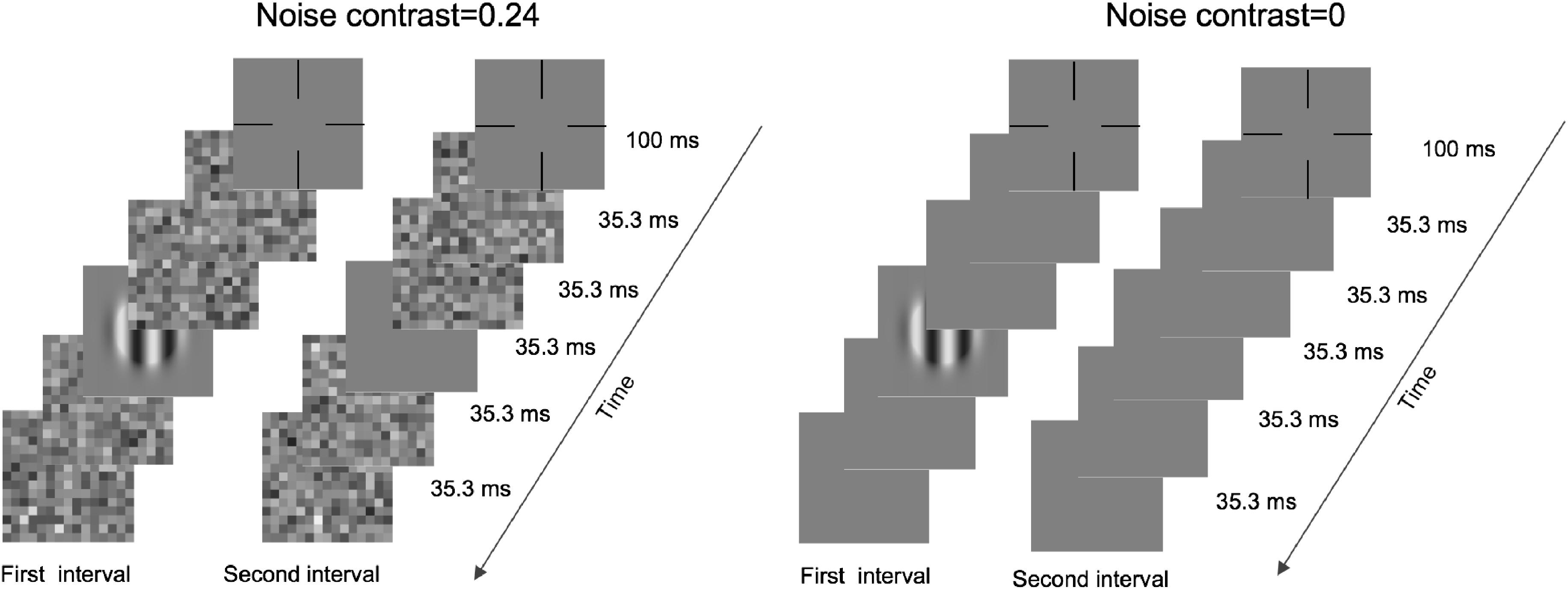
Figure 1. Illustration of a typical trial under high- (left) and zero- (right) noise conditions.
Design
The whole CSF test consisted of three noise levels (0, 0.12, and 0.24) and 10 spatial frequency conditions, which were measured by the qCSF procedure (Hou et al., 2010). The qCSF procedure was developed based on two critical assumptions as follows: (1) an individual CSF can be well fitted by a model with four parameters; (2) the slopes of psychometric functions do not depend on spatial frequency or external noise intensity (Rohaly and Owsley, 1993; Strasburger, 2001; Watson and Ahumada, 2005; Chen et al., 2014). The three noise levels were randomly mixed between trials. Each noise condition included 100 trials. The test sequences of two monocular conditions and one binocular condition were counterbalanced between subjects. For monocular testing, the non-tested eye was covered with an opaque occluder. To better evaluate the binocular gain, we computed the area under the log CSF (AULCSF, in log10 units), which served as the index of CS across all spatial frequencies (Koop et al., 1996; Zhang et al., 2018; Wu et al., 2020, 2021). For each subject, eyes with larger and smaller AULCSF were defined as good and bad eyes, respectively. The binocular summation ratio (BSR) was computed by the performance (AULCSF or CS) in the binocular condition divided by that of good (BSRG) or bad (BSRB) eyes.
Perceptual Template Model Model Analysis
In the PTM, the performance of a subject was calculated using the following equation:
where d′ denotes the performance; the equivalent internal additive and multiplicative noise is expressed by Nadd and Nmul, respectively; Next indicates the contrast of external noise; γ denotes the non-linearity of the system; β is the perceptual template gain; c presents the signal contrast. To model the effect of binocular summation on CS, Aa, Af, and Am were added in front of Nadd, Next, and Nmul, respectively. Under monocular conditions, Aa, Af, and Am were all set to 1. Because the slope was found to be constant between the binocular and any one of the two monocular conditions (see detailed analysis in Supplementary Information), the multiplicative noise was assumed to be constant and independent of the viewing condition. Thus, we removed Am from Equation 1 and only set Aa and Af free (Xu et al., 2006; Zhang et al., 2018). In addition, under different spatial frequency conditions, Na and β varied, but Nm and γ did not. In summary, two potential factors were considered to explain the binocular gain on CS: lower internal additive noise and a better perceptual template (the ability of the external noise filter). The full model assumed that binocular summation decreased internal additive noise and improved the perceptual template. The reduced model 1 assumed that binocular summation only decreased internal additive noise, and the reduced model 2 assumed that binocular summation only improved the perceptual template. The most reduced model assumed no changes in the parameters. The goodness of fit was calculated as follows:
where r2 is the index of the goodness of fit; and yi denote the predicted and original values, respectively; represents the mean of all original values. To select the best model, we performed an F-test to compare the r2 of the four models (Huang et al., 2010). The best-fitting model was the one that was statistically better than any reduced model but not significantly worse than the full model.
Results
The CSF at the three noise levels when using the good eye, the bad eye, and both eyes are plotted in Figure 2. A visual inspection suggested that the binocular CS was much better than any monocular CS, especially when external noise was absent. To briefly compare the CS between monocular and binocular conditions, the AULCSF is plotted (Figure 3). The AULCSF of the good eye (GE), bad eye (BE), and two eyes (TE) for the conditions was as follows: 6.527 ± 0.147, 5.842 ± 0.211, and 7.478 ± 0.15 (log10 unit, mean ± SE) under zero-noise conditions, respectively; 3.872 ± 0.328, 3.414 ± 0.288, and 4.212 ± 0.252 under low-noise conditions, respectively; 2.621 ± 0.254, 2.402 ± 0.226, and 2.815 ± 0.204 under high-noise conditions, respectively. A repeated measure ANOVA was conducted on the AULCSF with the eye and noise conditions as within-subject factors. The main effects of the eye and noise conditions and the interaction effect among them were all significant [F(2, 16) = 3.693, p < 0.001; F(2, 16) = 251.135, p < 0.001; F(4, 32) = 98.259, p < 0.001]. A simple-effect analysis revealed that: (1) when no noise was present, the AULCSF was largest in TE, followed by GE and BE (all, p < 0.05); (2) when low noise was present, the AULCSF was also largest in TE, followed by GE and in BE (all, p < 0.05); (3) when high noise was present, only the difference in the AULCSF between TE and BE reached marginal significance (p = 0.078). In summary, significant binocular CS dominance was observed, especially when zero or low noise was present.
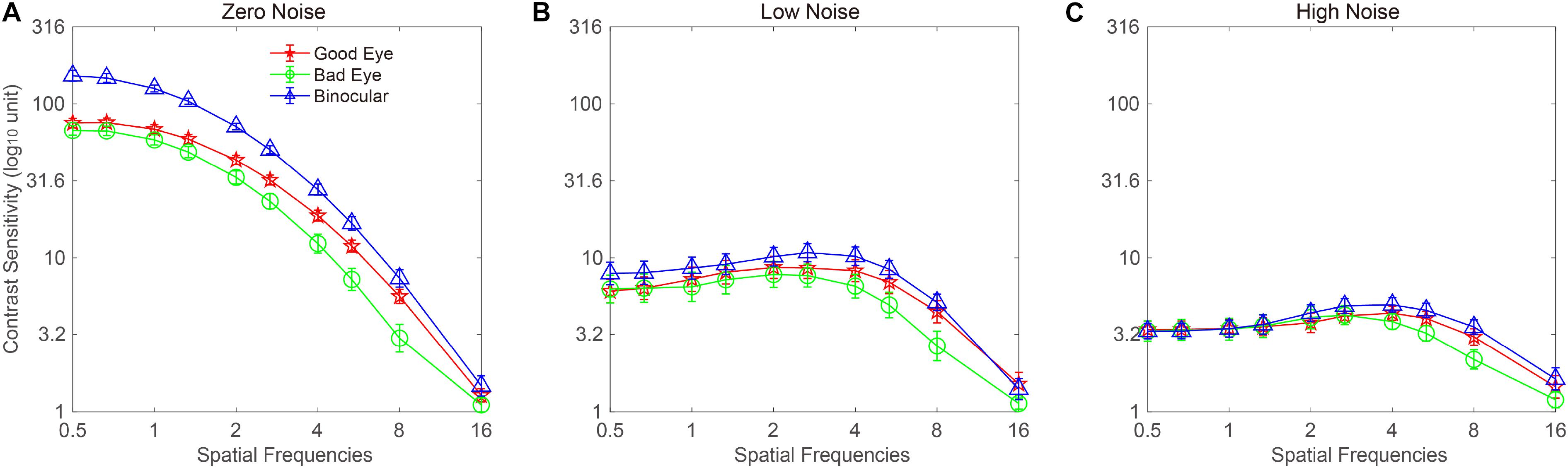
Figure 2. Monocular and binocular contrast sensitivity functions (CSFs) at (A) zero-, (B) low-, and (C) high-noise levels, respectively. Red lines with pentagram symbols, green lines with circle symbols, and blue lines with triangles denote contrast sensitivity (CS) when using the good eye (GE), bad eye (BE), and two eyes (TE), respectively. Data were averaged across subjects. The error bar denotes SE.
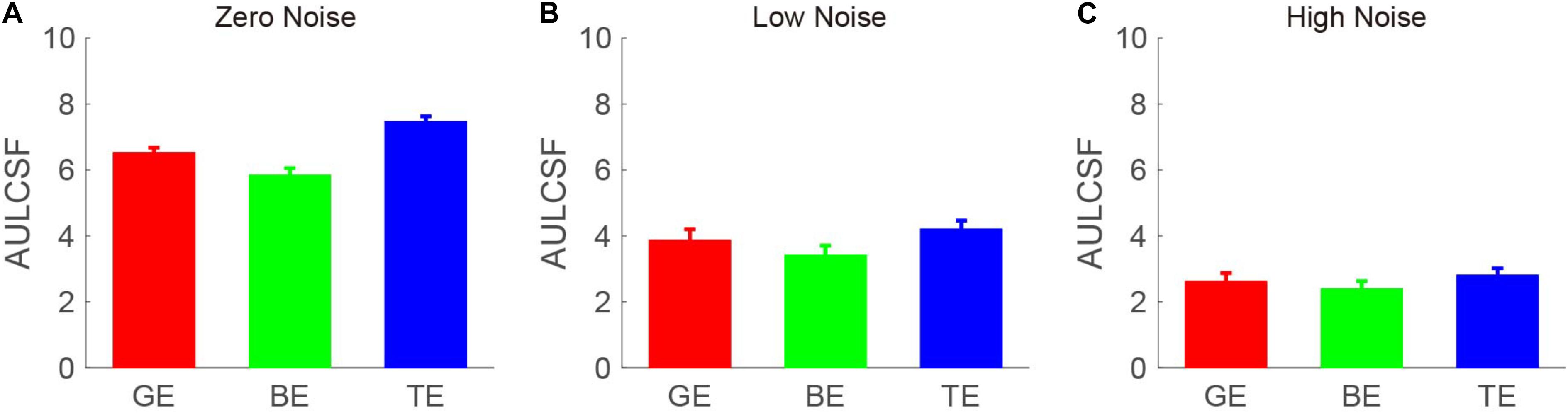
Figure 3. Area under the log CSF (AULCSF) (log10 units) under (A) zero-, (B) low-, and (C) high- (C) noise conditions. Red, green, and blue bars denote the data from GE, BE, and TE, respectively. The error bar denotes SE.
The BSR was computed by dividing the binocular AULCSF by the AULCSF of the “good eye” (BSRG) or “bad eye” (BSRB), respectively (Figure 4). The BSRG under zero-, low-, and high-noise conditions was 1.147 ± 0.018, 1.118 ± 0.047, and 1.131 ± 0.087, respectively. In contrast, the BSRB under zero-, low-, and high-noise conditions was 1.29 ± 0.040, 1.265 ± 0.075, and 1.228 ± 0.101, respectively. On average, the BSRB was greater than the BSRG across different noise conditions (1.261 ± 0.052 vs. 1.132 ± 0.045). To provide statistical results, a repeated ANOVA was performed on the summation ratios with the standard eye (good vs. bad) and noise conditions (zero, low, and high) as within-subject factors. The main effect of the standard eye conditions was significant, indicating that the summation ratio was significantly higher when the bad eye was considered as the standard eye [F(1, 8) = 6.485, p < 0.001]. However, the main effect of noise conditions and the interaction effect between standard eye and noise conditions failed to reach significance [F(2, 16) = 0.175, p = 0.841; F(2, 16) = 0.192, p = 0.827].
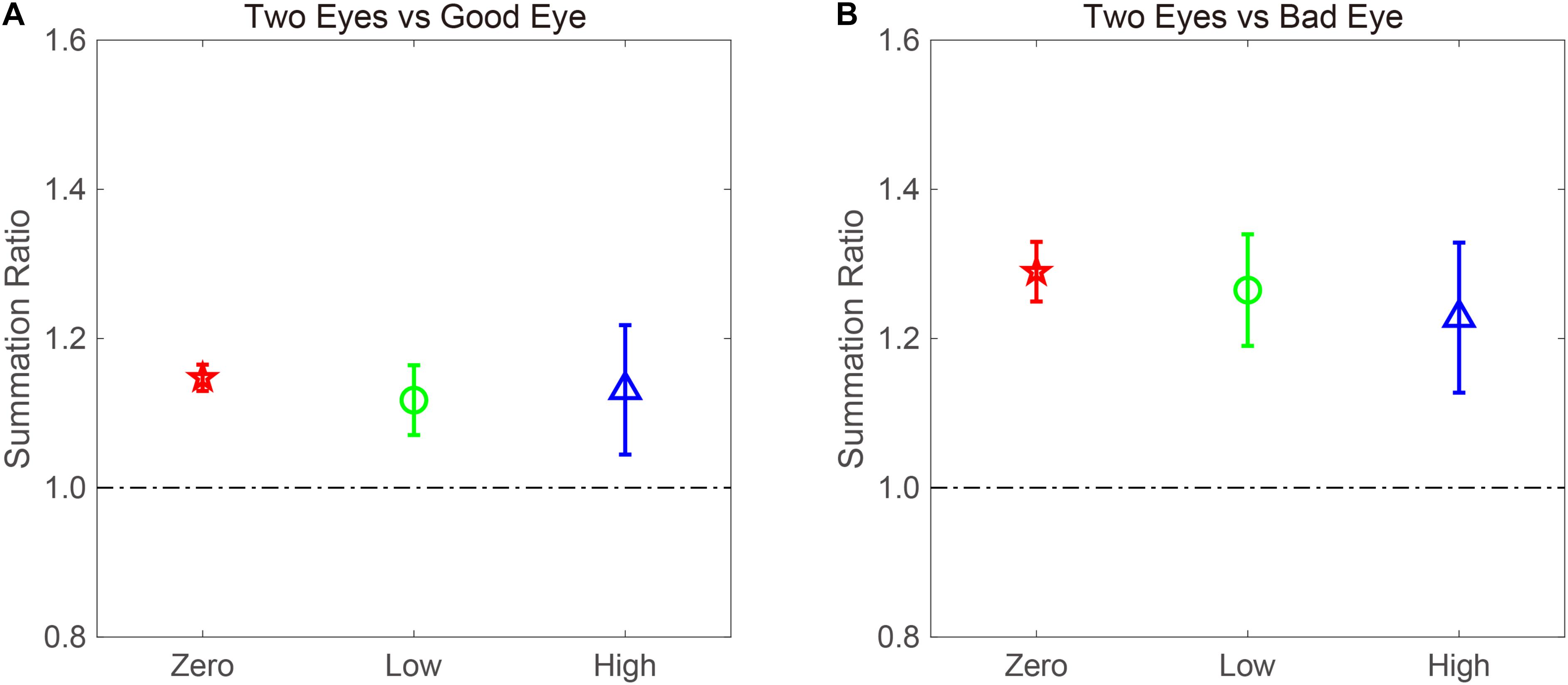
Figure 4. AULCSF-based binocular summation ratios (BSRs) when the (A) good and (B) bad eyes were considered as the standard eyes, respectively. Red, green, and blue colors denote the zero-, low-, and high-noise conditions, respectively. The error bar denotes SE.
Traditionally, a BSR with a value greater than 1 denotes binocular gain. However, if the BSR is smaller than 1, binocular loss or inhibition is indicated. Thus, it is quite necessary to confirm whether summation ratios were significantly different from 1. When the good eye was considered as the standard eye, a repeated analysis was conducted on the summation ratios to verify the difference between the three noise conditions and 1. We found that the main effect was marginally significant [F(3, 24) = 2.45, p = 0.088]. Least significant difference (LSD) test revealed that the summation ratios under zero- and low-noise conditions were significantly greater than 1 (all, p < 0.05), but that there was no difference between high-noise conditions and 1 (p = 0.169). When the bad eye was considered as the standard eye, the same analysis was conducted, and the results were similar. That is, the summation ratios under zero- and low-noise conditions were significantly greater than 1 (all, p < 0.05), but the difference between high-noise conditions and 1 reached marginal significance (p = 0.053). These findings suggested that external noise modulates the extent of binocular summation.
To examine whether the binocular summation effect is dependent on spatial frequency, we plotted the CS-based BSR vs. a spatial frequency curve (Figure 5). When calculating the summation ratio, 16 cpd may produce some extreme values, because CS could not be measured at a specific external noise level on some subjects. To exclude the influence of extreme values on the data analysis, the data at 16 cpd were not included. For the remaining data, we averaged the CS in different noise conditions and across subjects. The BSR when the good eye was considered as the standard eye is plotted in Figure 5A. A visual inspection suggested that the BSR under zero- and low-noise conditions was greater than 1 at all spatial frequencies. On average, the BSRs were 1.143 ± 0.003 and 1.098 ± 0.009 across spatial frequencies under zero- and low-noise conditions, respectively. In contrast, the BSR under high-noise conditions was only 1.056 ± 0.02 across spatial frequencies. However, the pattern in the high-noise condition suggested that binocular summation gain only existed at high spatial frequencies. Indeed, the BSRs were 0.996 ± 0.011 and 1.104 ± 0.009, at low (<2 cpd) and high (≥2 cpd) spatial frequencies, respectively.
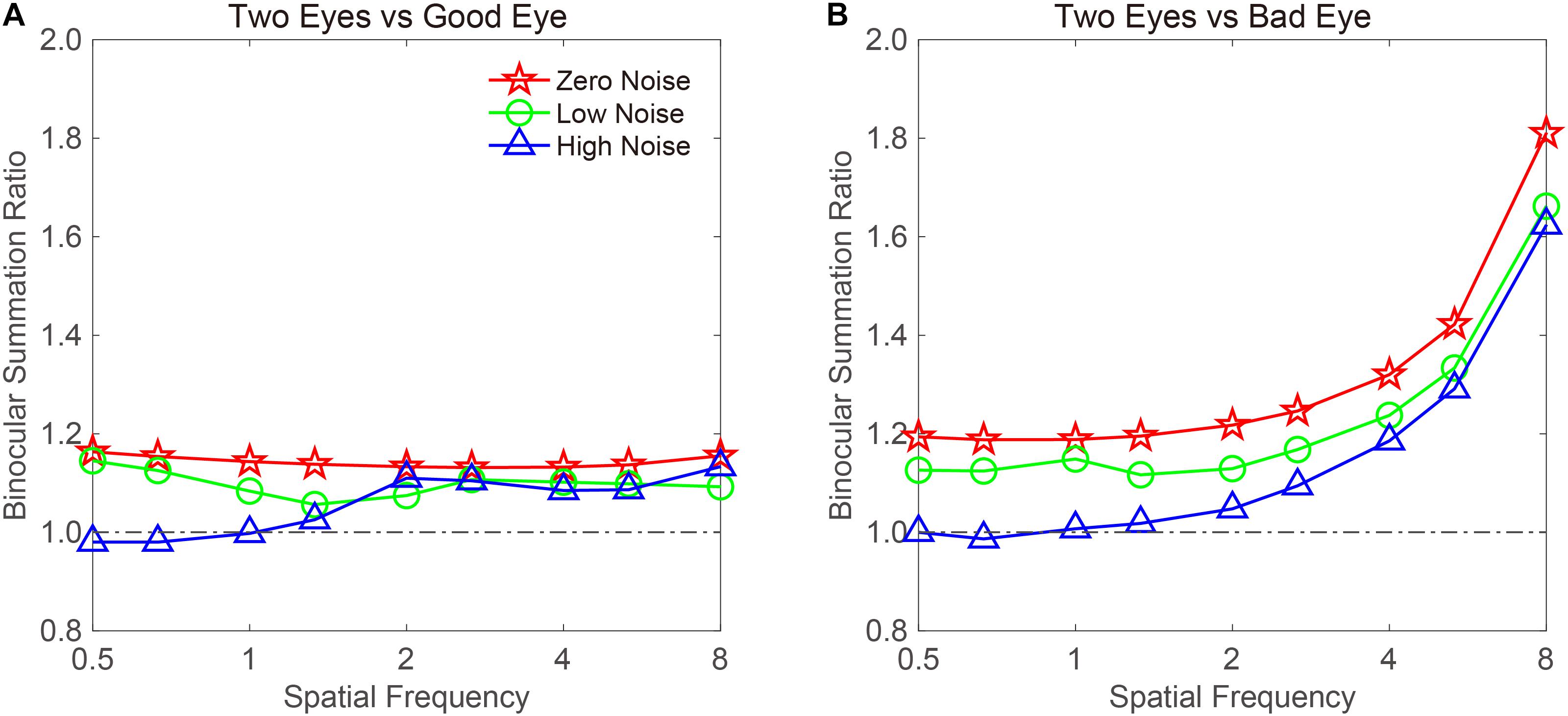
Figure 5. CS-based BSRs vs. a spatial frequency curve. Data were plotted when the (A) good or (B) bad eye was considered as the standard eye, respectively. Red, green, and blue colors denote the zero-, low-, and high-noise conditions, respectively.
When the bad eye was considered as the standard eye, the BSR vs. the spatial frequency curve was plotted (Figure 5B). The BSR curve started horizontally at low spatial frequencies and then increased with spatial frequency. Under zero-noise conditions, the BSRs were 1.191 ± 0.002 and 1.403 ± 0.108 at low (<2 cpd) and high (≥2 cpd) spatial frequencies, respectively. Under low-noise conditions, the BSRs were 1.129 ± 0.007 and 1.306 ± 0.096 at low (<2 cpd) and high (≥2 cpd) spatial frequencies, respectively. Under high-noise conditions, the BSRs were 1.003 ± 0.007 and 1.249 ± 0.103 at low (<2 cpd) and high (≥2 cpd) spatial frequencies, respectively. These findings indicated that the BSR is highly dependent on spatial frequency, but high noise decreases it.
To illustrate the mechanisms of binocular summation, the data were first averaged across subjects and then fitted with the PTM. The model with the least parameters while maintaining the significant effect of the binocular summation according to Equation 2 was selected as the best-fitting model. When the good eye was considered as the standard eye, the r2 of the full, reduced Model 1, reduced Model 2, and most reduced model was 96.3, 95, 87.2, and 86.8%, respectively. The full model was selected as the best-fitting model because it r2 was significantly higher than that of the reduced models (all, p < 0.05). On average, the Aa and Af in the full model were 0.572 ± 0.059 and 0.912 ± 0.034, respectively, across all spatial frequencies (Figure 6A). When the bad eye was considered as the standard eye, the r2of the full, reduced Model 1, reduced Model 2, and most reduced model was 95.4, 78, 76.3, and 71.2%, respectively. The full model was selected as the best-fitting model because it r2 was significantly higher than that of the reduced models (all, p < 0.05). On average, the Aa and Af in the full model were 0.34 ± 0.073 and 0.625 ± 0.055, respectively, across all spatial frequencies (Figure 6B). These results suggested that both decreased internal additive noise and the improved perceptual template contribute to the binocular summation.
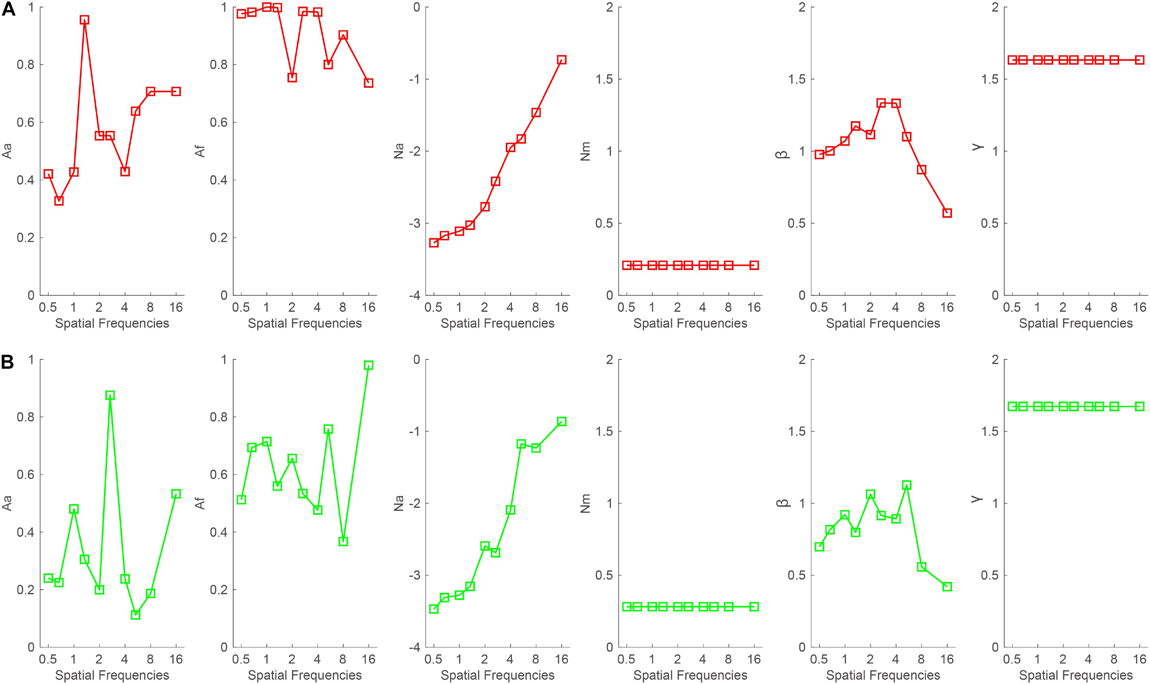
Figure 6. Aa, Af, Na, Nm, β, and γ as a function of spatial frequencies when the (A) good or (B) bad eye was considered as the standard eye, respectively.
Discussion
In this study, we explored the effect of external noise and spatial frequency on binocular CS summation and determined the corresponding mechanisms with a PTM. The binocular gain was observed, but its extent was strongly dependent on the standard eye, spatial frequency, and external noise conditions. The PTM analysis suggested that the internal additive noise was reduced and that the perceptual template was promoted under binocular viewing conditions.
The spatial frequency-dependent binocular summation gain has been investigated by previous studies, but our experimental design still provided significant innovation. First, the CSF was accessed through the qCSF method with high precision and efficiency (Lesmes et al., 2010). Approximately 500–1,000 trials are required by the traditional CSF measurement to produce a reasonable precision, which is time-consuming (Harvey, 1986). Thus, the qCSF method not only saves working time but also reduces fatigue in subjects. Second, due to the limitation of the traditional CSF assessment, some researchers only measured two spatial frequencies (Pardhan, 1996). In contrast, the CS over 10 spatial frequencies was obtained with the qCSF method. Thus, a clear pattern of the BSR vs. the spatial frequency curve was observed, and the binocular summation gain was evaluated by both CS and AULCSF.
The external noise level-dependent BSR was another highlight of this study. First, based on the AULCSF, the BSR was greatest under zero-noise conditions, followed by low-noise and high-noise conditions. In addition, with high external noise, there was a greater individual difference in the BSR. Second, based on the CS, the BSRB increased with spatial frequencies regardless of external noise levels. In contrast, the BSRG was dependent on a spatial frequency only when high external noise was present.
Binocular summation ratios have been investigated by many studies (Frisén and Lindblom, 1988; Pardhan, 1996, 1997; Thylefors and Havelius, 2014). In most of these studies, the BSR is between 0 and 100%, largely depending on which visual task is studied. The BSRs in this study were lower than those determined with the contrast detection task. For example, when considering the good eye as the standard eye, the BSR in our study was 1.19 and 1.2 at 1 and 5.3 cpd, respectively. In contrast, Pardhan (1996) reported that the BSR was 1.45 and 2.26 at 1 and 5.3 cpd, respectively. This difference may be due to different experimental settings, e.g., stimuli size, duration time, and screen luminance. Pardhan and Shahia did not report the details of their duration time. The duration time in the current study was 33.3 ms, which was short. Thus, it will be quite interesting to examine the effect of duration time on the BSR in the future.
With the help of the PTM, we found that lower internal noise and a better perceptual template characterized the binocular summation gain. In addition, when the bad eye was considered as the standard eye, the changes in internal noise and perceptual template were much more pronounced than those when the good eye was considered the standard eye. These results were expected because the extent of the binocular gain was much greater when the bad eye was considered as the standard eye. Interestingly, the extent of the changes in internal noise was greater than that in the perceptual template, implying that the changes in internal noise are the dominant mechanism.
In this study, the grating size was varied with spatial frequencies. Although there may be a concern that CS is attributed to grating size instead of spatial frequency, there is evidence to suggest otherwise. First, Pelli and Bex suggested that the use of a fixed number of sinewave cycles is much better because neurons in the visual cortex are roughly spatial scale-invariant (Pelli and Bex, 2013). Second, when fixing the grating size, increasing spatial frequency may induce additional processes, e.g., spatial summation (Jamar and Koenderink, 1983). Third, the stimuli with fixed cycles have been used in many previous studies (Xu et al., 2006; Chen et al., 2014; Hou et al., 2015; Li et al., 2015; Zheng et al., 2018, 2019; Yan et al., 2020). Furthermore, fixing the cycles of grating maintains the spectral relationship between the signal and external noise remained identical under all the spatial frequency conditions. Thus, these studies suggest that the present experimental setting is rigorous.
The improvement of the binocular summation gain is an interesting research topic. A previous study has found that patients with large interocular CS differences, such as amblyopia (Pardhan and Whitaker, 2000), produced a low efficiency of binocular summation. The improvement in the visual function of the amblyopic eye by perceptual learning (Huang et al., 2008; Xie and Yu, 2018) or transcranial direct current stimulation (Ding et al., 2016) has been demonstrated. However, it is still unknown whether or how much the efficiency of binocular summation could be restored. The qCSF method with multiple external noise levels has great implications for the recovery of patients with ocular conditions, especially when they participate in a visual task in an extreme environment, e.g., external noise.
Data Availability Statement
The original contributions presented in the study are included in the article/Supplementary Material, further inquiries can be directed to the corresponding author/s.
Ethics Statement
The studies involving human participants were reviewed and approved by the Ethical Review Committee of Hebei Normal University. The patients/participants provided their written informed consent to participate in this study.
Author Contributions
PZ, DW, and ZW designed the experiment and wrote the manuscript. PZ collected and analyzed the data. PZ, DW, HW, WR, QL, GC, CL, JT, SZ, and YL revised the manuscript. All authors contributed to the article and approved the submitted version.
Funding
This work was supported by the Social Science Foundation of Hebei Province (HB20JY020 and HB14JY031 to ZW), Natural Science Foundation of Hebei Province (C2012205046 to ZW and C2021205005 to PZ), and University-Level Scientific Research Project in CDMC (202113 to JT).
Conflict of Interest
The authors declare that the research was conducted in the absence of any commercial or financial relationships that could be construed as a potential conflict of interest.
Publisher’s Note
All claims expressed in this article are solely those of the authors and do not necessarily represent those of their affiliated organizations, or those of the publisher, the editors and the reviewers. Any product that may be evaluated in this article, or claim that may be made by its manufacturer, is not guaranteed or endorsed by the publisher.
Supplementary Material
The Supplementary Material for this article can be found online at: https://www.frontiersin.org/articles/10.3389/fpsyg.2021.740759/full#supplementary-material
References
Alberti, C., and Bex, P. (2018). Binocular contrast summation and inhibition depends on spatial frequency, eccentricity and binocular disparity. Ophthalmic Physiol. Opt. 38, 525–537. doi: 10.1111/opo.12581
Blake, R., and Fox, R. (1973). The psychophysical inquiry into binocular summation. Percept. Psychophys. 14, 161–185. doi: 10.3758/BF03198631
Campbell, F. W. (1983). Why do we measure contrast sensitivity? Behav. Brain Res. 10, 87–97. doi: 10.1016/0166-4328(83)90154-7
Campbell, F. W., and Green, D. G. (1965). Monocular versus binocular visual acuity. Nature 208, 191–192. doi: 10.1038/208191a0
Chen, G., Hou, F., Yan, F.-F., Zhang, P., Xi, J., Zhou, Y., et al. (2014). Noise provides new insights on contrast sensitivity function. PLoS One 9:e90579. doi: 10.1371/journal.pone.0090579
Crawford, M., and Cool, S. J. (1970). Binocular stimulation and response variability of striate cortex units in the cat. Vis. Res. 10, 1145–1153. doi: 10.1016/0042-6989(70)90031-3
Ding, Z., Li, J., Spiegel, D. P., Chen, Z., Chan, L., Luo, G., et al. (2016). The effect of transcranial direct current stimulation on contrast sensitivity and visual evoked potential amplitude in adults with amblyopia. Sci. Rep. 6:19280. doi: 10.1038/srep19280
Dosher, B. A., and Lu, Z.-L. (1998). Perceptual learning reflects external noise filtering and internal noise reduction through channel reweighting. Proc. Natl. Acad. Sci. U S A. 95, 13988–13993. doi: 10.1073/pnas.95.23.13988
Frisén, L., and Lindblom, B. (1988). Binocular summation in humans: evidence for a hierarchic model. J. Physiol. 402, 773–782. doi: 10.1113/jphysiol.1988.sp017233
Harvey, L. (1986). Efficient estimation of sensory thresholds. Behav. Res. Methods Instruments Comp. 18, 623–632. doi: 10.3758/BF03201438
Home, R. (1978). Binocular summation: a study of contrast sensitivity, visual acuity and recognition. Vis. Res. 18, 579–585. doi: 10.1016/0042-6989(78)90206-7
Hou, F., Huang, C.-B., Lesmes, L. A., Feng, L.-X., Tao, L., Zhou, Y.-F., et al. (2010). qCSF in clinical application: efficient characterization and classification of contrast sensitivity functions in amblyopia. Invest. Ophthalmol. Vis. Sci. 51, 5365–5377. doi: 10.1167/iovs.10-5468
Hou, F., Lesmes, L. A., Bex, P., Dorr, M., and Lu, Z.-L. (2015). Using 10AFC to further improve the efficiency of the quick CSF method. J. Vis. 15:2. doi: 10.1167/15.9.2
Huang, C.-B., Zhou, J., Zhou, Y., and Lu, Z.-L. (2010). Contrast and phase combination in binocular vision. PLoS One 5:e15075. doi: 10.1371/journal.pone.0015075
Huang, C.-B., Zhou, Y., and Lu, Z.-L. (2008). Broad bandwidth of perceptual learning in the visual system of adults with anisometropic amblyopia. Proc. Natl. Acad. Sci. U S A. 105, 4068–4073. doi: 10.1073/pnas.0800824105
Jamar, J., and Koenderink, J. J. (1983). Sine-wave gratings:Scale invariance and spatial integration at suprathreshold contrast. Vis. Res. 23, 805–810. doi: 10.1016/0042-6989(83)90203-1
Koop, M. R., Applegate, R., and Howland, H. C. (1996). Changes in the area under the log contrast sensitivity function (AULCSF) with myopic refractive error. Invest. Ophthalmol. Vis. Sci. 37, 1482–1482.
Lesmes, L. A., Lu, Z.-L., Baek, J., and Albright, T. D. (2010). Bayesian adaptive estimation of the contrast sensitivity function: the quick CSF method. J. Vis. 10, 17.1–21. doi: 10.1167/10.3.17
Li, C. Y., and Creutzfeldt, O. (1984). The representation of contrast and other stimulus parameters by single neurons in area 17 of the cat. Pflügers Arch. 401, 304–314. doi: 10.1007/BF00582601
Li, L., Yu, Y., and Zhou, Y. (2015). The unilateral mean luminance alters additive internal noise in normal vision. Perception 44, 1215–1224. doi: 10.1177/0301006615594907
Lu, Z.-L., and Dosher, B. A. (2008). Characterizing observers using external noise and observer models: assessing internal representations with external noise. Psychol. Rev. 115, 44–82. doi: 10.1037/0033-295X.115.1.44
Ohzawa, I., and Freeman, R. D. (1986). The binocular organization of simple cells in the cat’s visual cortex. J. Neurophysiol. 56, 243–259. doi: 10.1152/jn.1986.56.1.221
Pardhan, S. (1996). A comparison of binocular summation in young and older patients. Curr. Eye. Res. 15, 315–319.
Pardhan, S. (1997). A comparison of binocular summation in the peripheral visual field in young and older patients. Curr. Eye Res. 16, 252–255. doi: 10.1076/ceyr.16.3.252.15407
Pardhan, S., and Elliott, D. B. (1991). Clinical measurements of binocular summation and inhibition in patients with cataract. Clin. Vis. Sci. 6, 355–359.
Pardhan, S., and Gilchrist, J. (1990a). Binocular contrast sensitivity with monocular glare disability. Ophthalmic Physiol. Opt. 10, 37–39. doi: 10.1016/0275-5408(90)90128-L
Pardhan, S., and Gilchrist, J. (1990b). The effect of monocular defocus on binocular contrast sensitivity. Ophthalmic Physiol. Opt. 10, 33–36. doi: 10.1016/0275-5408(90)90127-K
Pardhan, S., and Whitaker, A. (2000). Binocular summation in the fovea and peripheral field of anisometropic amblyopes. Curr. Eye Res. 20, 35–44.
Pelli, D. G. (1997). The videotoolbox software for visual psychophysics: transforming numbers into movies. Spatial Vis. 10, 437–442. doi: 10.1163/156856897X00366
Pelli, D. G., and Bex, P. (2013). Measuring contrast sensitivity. Vis. Res. 90, 10–14. doi: 10.1016/j.visres.2013.04.015
Rohaly, A. M., and Owsley, C. (1993). Modeling the contrast-sensitivity functions of older adults. J. Opt. Soc. Am. Opt. Image Sci. 10:1591. doi: 10.1364/JOSAA.10.001591
Rubin, G. S., West, S. K., Muoz, B., Bandeen-Roche, K., and Fried, L. P. (1997). A comprehensive assessment of visual impairment in a population of older Americans. the see study. salisbury eye evaluation project. Invest. Ophthalmol. Vis. Sci. 38, 557–568.
Strasburger, H. (2001). Invariance of the psychometric function for character recognition across the visual field. Percept. Psychophys. 63, 1356–1376. doi: 10.3758/BF03194548
Thylefors, J., and Havelius, U. (2014). Two eyes are better than one—binocular summation of dark vision in healthy individuals and patients with chronic respiratory disease. Neuro-Ophthalmology 38, 113–121. doi: 10.3109/01658107.2013.879599
Watson, A. B., and Ahumada, A. J. (2005). A standard model for foveal detection of spatial contrast. J. Vis. 5, 717–740. doi: 10.1167/5.9.6
Wu, D., Liu, N., Xu, P., Sun, K., Xiao, W., and Li, C. (2020). Reduced contrast sensitivity function in central and peripheral vision by disability glare. Perception 49, 1348–1361. doi: 10.1177/0301006620967641
Wu, D., Zhou, Y., Lv, H., Liu, N., and Zhang, P. (2021). The initial visual performance modulates the effects of anodal transcranial direct current stimulation over the primary visual cortex on the contrast sensitivity function. Neuropsychologia 156:107854. doi: 10.1016/j.neuropsychologia.2021.107854
Xi, J., Zhang, P., Jia, W.-L., Chen, N., Yang, J., Wang, G.-T., et al. (2020). Multi-Stage cortical plasticity induced by visual contrast learning. Front. Neurosci. 14:555701. doi: 10.3389/fnins.2020.555701
Xie, X.-Y., and Yu, C. (2018). Double training downshifts the threshold vs. noise contrast (TvC) functions with perceptual learning and transfer. Vis. Res. 152, 3–9. doi: 10.1016/j.visres.2017.12.004
Xu, P., Lu, Z.-L., Qiu, Z., and Zhou, Y. (2006). Identify mechanisms of amblyopia in Gabor orientation identification with external noise. Vis. Res. 46, 3748–3760. doi: 10.1016/j.visres.2006.06.013
Yan, F.-F., Hou, F., Lu, H., Yang, J., Chen, L., Wu, Y., et al. (2020). Aging affects gain and internal noise in the visual system. Sci. Rep. 10:6768. doi: 10.1038/s41598-020-63053-0
Zhang, P., Hou, F., Yan, F.-F., Xi, J., Lin, B.-R., Zhao, J., et al. (2018). High reward enhances perceptual learning. J. Vis. 18:11. doi: 10.1167/18.8.11
Zheng, H., Shen, M., He, X., Cui, R., Lesmes, L. A., Lu, Z.-L., et al. (2019). Comparing spatial contrast sensitivity functions measured with digit and grating stimuli. Trans. Vis. Sci. Technol. 8:16. doi: 10.1167/tvst.8.6.16
Keywords: contrast sensitivity, binocular summation, internal additive noise, perceptual template, spatial frequency
Citation: Zhang P, Wang H, Ren W, Lu Q, Li C, Chen G, Zhang S, Tao J, Li Y, Wu D and Wang Z (2021) Lower Internal Additive Noise and Better Perceptual Template Characterize Binocular Contrast Sensitivity Summation. Front. Psychol. 12:740759. doi: 10.3389/fpsyg.2021.740759
Received: 13 July 2021; Accepted: 06 September 2021;
Published: 30 September 2021.
Edited by:
Yang Zhang, Soochow University, ChinaReviewed by:
Huazhan Yin, Hunan Normal University, ChinaLihong Chen, Liaoning Normal University, China
Copyright © 2021 Zhang, Wang, Ren, Lu, Li, Chen, Zhang, Tao, Li, Wu and Wang. This is an open-access article distributed under the terms of the Creative Commons Attribution License (CC BY). The use, distribution or reproduction in other forums is permitted, provided the original author(s) and the copyright owner(s) are credited and that the original publication in this journal is cited, in accordance with accepted academic practice. No use, distribution or reproduction is permitted which does not comply with these terms.
*Correspondence: Di Wu, d3VkaTA0MjZAb3V0bG9vay5jb20=; Zeng Wang, d2FuZ3plbmdAaGVibXUuZWR1LmNu