GNSS interference mitigation method based on deep learning

The interference environment faced by GNSS receivers is unknown, dynamic, and uncertain, making it difficult for a single interference mitigation method to address all interference threats. In this paper, we introduce an intelligent interference mitigation approach. By leveraging a deep learning network model, our method automatically selects the optimal interference mitigation technique based on the specific characteristics of the interference. This enhances the receiver’s anti-jamming performance and overall robustness. Our experimental results show that the proposed method effectively suppresses narrowband interference, pulse interference, and chirp interference, demonstrating insensitivity to interference parameters. Statistically, it outperforms traditional methods, with the proportion of the carrier-to-noise ratio (C/N₀) above a given threshold (initial C/N₀ reduced by 3 dB) increasing by over 10%.

1 Introduction

Global Navigation Satellite Systems (GNSS) provide users with positioning, velocity, and timing (PVT) services. It is the only positioning and navigation system that offers high precision, global coverage, and all-weather availability. After decades of development, GNSS has been widely and deeply applied across various sectors.

Because GNSS plays a fundamental and key role in military, commercial and civil fields, its vulnerability has also received more and more attention. As we all know, the power of the signal emitted by the navigation satellite is very weak when it reaches the ground, and GNSS users are extremely vulnerable to radio frequency interference and spoofing attacks [1, 2]. Studies have shown that [3] an interference source with a radiation power of only 1 W can render GNSS receivers within a range of approximately 15 km unable to function properly.

Radio frequency interference can be categorized into unintentional and intentional interference. Unintentional interference is generally caused by spectrum leakage or improper operation of radar or communication systems adjacent to the navigation frequency band. Intentional interference is typically used to attack an opponent’s navigation equipment or to protect one’s privacy [4]. Typical GNSS interference includes continuous wave interference, narrowband interference, pulse interference, sweep chirp interference and broadband interference [5–7]. The impact of different types of interference on GNSS receivers can be quantitatively characterized by the equivalent C/N₀ [8].

To address the threat of radio frequency interference, researchers have proposed a series of interference suppression methods. The basic principle is similar: utilizing the sparsity of interference in a certain dimension to detect and eliminate it. For example, due to the sparsity of continuous wave interference and narrowband interference in the frequency domain, Frequency Domain Pulse Blanking (FDPB) and Adaptive Filtering (AF) [9–12] have been proposed for suppression. In light of the sparsity of pulse interference in the time domain, Time Domain Pulse Blanking (TDPB) [13, 14] has been proposed for suppression. For chirp interference, it has been found that [15, 16] it also exhibits time-domain sparsity within a specific sweep frequency range, allowing it to be suppressed by setting the time-domain pulse to zero. Broadband interference is unique in that it does not exhibit sparsity in either the time or frequency domains; it must be received by an array antenna or polarized antenna to demonstrate sparsity in the spatial or polarization domain for suppression. This paper does not address broadband interference.

The interference mitigation method of radio frequency has been a topic not only in electronics but also in space and astrophysics. Among these, deep learning methods were already employed. References [17–19] investigate how to detect and identify radio-frequency interference using deep learning methods, which have achieved good results in the field of radio interferometry. However, these methods do not provide further approaches for interference cancellation or signal recovery. References [20, 21] study the use of Bayesian methods to eliminate interference and restore signals. This method performs well under the condition that the prior distribution of the data is known. However, the interference faced by GNSS receiver is unknown, dynamic, and uncertain. Moreover, under different types of interference, the data exhibit different probability distributions. Therefore, it is difficult to directly apply this method in GNSS interference mitigation. For a given type of interference, different mitigation methods yield varying suppression effects. This paper aims to design an interference mitigation method that not only identifies interference, but also automatically selects the optimal approach to suppress interference based on its characteristics, thereby enhancing the performance and robustness of the receiver. This method is referred to as the intelligent interference mitigation (IIM) method.

The innovative contributions of this paper can be summarized as follows: (a) We propose a GNSS IIM method that utilizes spectrum sensing to convert input data into spectrograms, followed by the application of a deep learning network to output the optimal interference mitigation method. (b) We present an implementation framework for the IIM method, which employs Short Time Fourier Transform (STFT) for time-frequency two-dimensional spectral sensing, with GoogLeNet chosen as the pre-trained model to build our deep learning network. (c) Finally, we conduct experiments using a data collector and a software-defined receiver (SDR) for interference mitigation and signal processing to evaluate the performance of the proposed method under various interference conditions. The results demonstrate the effectiveness of the proposed method and its ability to mitigate different types of interfering signals.

The content of this article is organized as follows: Section 2 establishes the signal model for the GNSS receiver; Section 3 introduces three typical GNSS interference mitigation methods—FDPB, AF, and TDPB—and analyzes their interference suppression effects. Section 4 proposes the basic principles and implementation framework of the GNSS IIM method. Sections 5, 6 design simulations and open-sky experiments to verify the performance of the proposed method. Finally, the main conclusions drawn from this study are presented.

2 Signal model

For the sake of simplicity, we consider the reception of a single GNSS satellite signal due to the very low cross-correlation of the pseudorandom spreading codes. The signal received by a GNSS receiver, after being amplified, down-converted, filtered, and sampled, can be expressed in complex baseband form as:

$x\left(n\right)=\sqrt{2P_s}d\left(n-{\tau }_0\right)p\left(n-{\tau }_0\right)e^{j\left(2\pi f_{0}n+{\phi }_0\right)}+\eta \left(n\right)+i\left(n\right)(1)$

Where $P_s$ is the power of the GNSS signal, $d\left(n\right)$ is the navigation information modulated in the signal, $p\left(n\right)$ is the pseudo-random code sequence, $f_0$ is the Doppler frequency shift, ${\tau }_0$ and ${\phi }_0$ are the pseudo-code phase and the carrier phase respectively, n is the time subscript. $i\left(n\right)$ is a generalized interference signal, and different interference types have different expressions [4]. $\eta \left(n\right)$ is the zero mean additive white Gaussian noise (AWGN) in the complex form. The real part and the imaginary part are independent and identically distributed. The variance is ${\sigma }^2$, which can be described by Equation 2 as follows:

${\sigma }^2=N_0{B}_{fe}(2)$

Where $N_0$ is the noise spectral density, $B_{fe}$ is the receiver front-end bandwidth.

When the receiver adopts active interference mitigation processing, the generalized interference mitigation process can be modeled by Equation 3 as follows:

$y\left(n\right)=\mathrm{{\rm H}}\left[x\left(n\right)\right](3)$

In Equation 4, $y\left(n\right)$ is the interference mitigation output, $\mathrm{{\rm H}}\left[\cdot \right]$ represents a certain mathematical transformation, different interference mitigation methods have different mathematical transformation forms, which will be introduced in detail in Section 3.

After that, the receiver further performs correlation despreading on the anti-jamming output. The goal is to estimate the Doppler frequency shift and pseudo-code phase of the GNSS signal. This process can be achieved by maximizing the ambiguity function [8]:

$\widehat{f},\widehat{\tau }=\underset{f,\tau }{\mathrm{arg\; max}}\left|C\left(f,\tau \right)\right|=\underset{f,\tau }{\mathrm{arg\; max}}\left|{\displaystyle \sum _{n=1}^M}y\left(n\right)p\left(n-\tau \right)e^{-j2\pi fn}\right|(4)$

In Equation 4, $C\left(f,\tau \right)$ is the ambiguity function, the symbol “argmax” is a mathematical notation used to describe the argument that maximizes a given function or expression. In the above equation, $\underset{f,\tau }{\mathrm{arg\; max}}\left|C\left(f,\tau \right)\right|$ are the value of $f$ and $\tau$ that make $\left|C\left(f,\tau \right)\right|$ as large as possible. $\widehat{f}$ and $\widehat{\tau }$ are the estimated values of the doppler frequency shift and pseudo-code phase, respectively. M is the length of the sampled data used for the correlation despreading processing, and the corresponding signal duration is $T=M/f_s$, where $f_s$ is the sampling rate. This formula describes the relationship between the ambiguity function and the doppler frequency shift as well as the pseudo-code phase. The value of the ambiguity function is maximized when the estimated values of the doppler frequency shift and pseudo-code phase are equal to that of the input GNSS signal.

The purpose of anti-jamming is to suppress the interfering signals and retain the useful signal to the greatest extent. The effect can be evaluated by the C/N₀ after correlation dispreading, which can be described by Equation 5 as follows:

$C/N_0=\frac{1}{T}\cdot \frac{{\left|E\left\{C\left(\widehat{f},\widehat{\tau }\right)\right\}\right|}^2}{Var\left\{C\left(\widehat{f},\widehat{\tau }\right)\right\}}(5)$

where $E\left\{\cdot \right\}$ represents the mean value and $Var\left\{\cdot \right\}$ represents the variance.

3 Traditional GNSS interference mitigation methods

Without considering special forms of receiving antennas such as array antennas or polarized antennas, conventional GNSS receivers employ three representative interference mitigation methods: FDPB, AF, or TDPB. The following sections introduce each method separately.

3.1 FDPB

The FDPB method first transforms the signal into the frequency domain through discrete Fourier transform (DFT):

$X\left(k\right)={\displaystyle \sum _{n=0}^{N-1}}x\left(n\right)e^{-j2\pi \frac{kn}{N}}(6)$

In Equation 6, $X\left(k\right)$ is the frequency spectrum after the signal is transformed to the frequency domain, and N is the length of the DFT operation. At this time, if the interference is sparse in the frequency domain, it will be pulse-like distribution. It could be mitigated by setting a threshold and removing spectral lines with amplitudes exceeding the threshold. How to set a threshold has always been a difficult problem in engineering implementation. This method requires prior information such as receiver noise power and is difficult to adapt to changes in receiver noise background.

Borio et al. [9] proposes a more robust method:

$Y\left(k\right)=\frac{X\left(k\right)}{\left|X\left(k\right)\right|}(7)$

In Equation 7, $Y\left(k\right)$ is the spectrum after the interference spectrum line is eliminated. This method is a threshold-free method and does not depend on any prior information.

Finally, the interference eliminated spectrum is transformed back from the frequency domain to the time domain through inverse discrete Fourier transform (IDFT) to obtain interference mitigation output, which can be described by Equation 8:

$y\left(n\right)=\frac{1}{N}{\displaystyle \sum _{k=0}^{N-1}}Y\left(k\right)e^{j2\pi \frac{kn}{N}}(8)$

3.2 AF

AF can be achieved using finite impulse response (FIR) or infinite impulse response (IIR) filters, which can adaptively adjust coefficients based on certain algorithms and automatically form zeros in the frequency band where interference occurs, thereby achieving interference suppression. Considering that FIR filters are more robust than IIR filters, this paper adopts adaptive FIR filters.

Assuming the length of the FIR filter is L, the signal filtered by the FIR filter can be described as [11]:

$y\left(n\right)={\displaystyle \sum _{k=0}^{L-1}}x\left(n-k\right)h^{\left(n\right)}\left(L-k\right)(9)$

In Equation 9, $h^{\left(n\right)}\left(k\right)$ is the kth coefficient of FIR filter at time n. This formula describes the response of the signal x(n) after passing through an FIR digital filter.

The coefficients of the FIR filter can be updated using the Normalized Least-Mean-Square (NLMS) algorithm [11]:

$h^{\left(n+1\right)}\left(k\right)=h^{\left(n\right)}\left(k\right)-\frac{\mu }{{\left|x\left(n\right)\right|}^2}x\left(n\right){\left(y\left(n\right)\right)}^{*}(10)$

In Equation 10, $\mu$ is the normalization step factor, and ${\left(\cdot \right)}^{*}$ represents the conjugate operation. The coefficients update is driven by the error which is also the output y(n). The error represents the difference between the desired output and the actual output of the filter. The NLMS algorithm adjusts the learning rate through the normalized step factor $\mu$, the value of which directly affects the convergence speed and steady-state error of the algorithm. A larger $\mu$ value can make the algorithm converge faster, but may lead to a larger steady-state error, a smaller value will make the algorithm converge more slowly, but with a smaller steady-state error. The value of $\mu$ needs to be a trade-off between convergence speed and steady-state error, in the subsequent experiments, we empirically choose 0.1 as the value for $\mu$.

3.3 TDPB

The TDPB directly processes the sampled data, and the threshold-free method is also used here. The process can be described by Equation 11 as follows [9]:

$y\left(n\right)=\frac{x\left(n\right)}{\left|x\left(n\right)\right|}(11)$

3.4 Analysis of suppression performance on different interfering signals

We have constructed a MATLAB simulation platform consisting of a signal generator and a SDR, employing the Monte Carlo simulation method to analyze the performance of interference suppression. The analysis focuses on the effectiveness of traditional anti-jamming methods against three types of interference: narrowband (continuous wave interference can be considered as a special form of narrowband interference), pulse, and chirp. The configuration of the simulation platform is illustrated in the Figure 1.

Figure 1

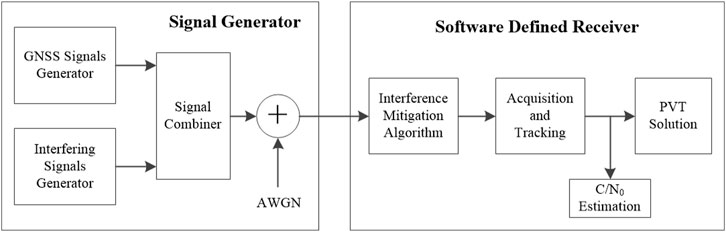
Figure 1. Simulation configuration.

The main parameter settings in the simulation are shown in the table below.

3.4.1 Narrowband interference suppression performance

Set the narrowband interference bandwidth to be randomly distributed between 0 and 4 MHz (20% signal bandwidth), simulate narrowband interference with different bandwidths, and use three methods of FDPB, AF, and TDPB for interference mitigation processing. Conduct 500 Monte Carlo experiments, obtain 500 samples, and statistically analyze the output C/N₀. The results are as follows:

Figure 2A shows the C/N₀ results of the first 30 experiments in 500 Monte Carlo simulations. It can be seen that the interference suppression performance of the AF algorithm is similar to that of the FDPB algorithm. The C/N₀ obtained by the AF algorithm is slightly higher than that of the FDPB algorithm in most cases, but also slightly lower than that of the FDPB algorithm in a few samples. The TDPB algorithm has a poor suppression effect on narrowband interference, and its output C/N₀ is generally lower than 30 dB Hz. Figure 2B shows the statistical results of 500 Monte Carlo experiments, with the horizontal axis representing the C/N₀ threshold and the vertical axis representing the proportion of experiments with a C/N₀ exceeding the given threshold to the total number of experiments. Figure 2B statistically illustrates that the AF algorithm has the best suppression effect on narrowband interference, followed by the FDPB algorithm and the TDPB algorithm.

Figure 2

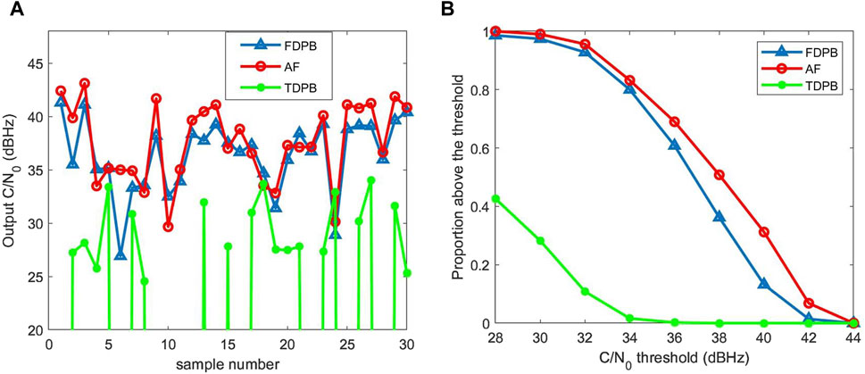
Figure 2. Comparison of narrowband interference suppression performance. (A) C/N₀ results of the first 30 experiments. (B) Statistical results of C/N₀ of 500 experiments.

3.4.2 Pulse interference suppression performance

The pulse repetition period of pulse interference is randomly distributed between 0.04 and 1 ms, and the duty cycle is randomly distributed between 0 and 0.4 (Gaussian band-limited noise modulated within pulse signals). The bandwidth covers the entire front-end bandwidth of the receiver (20 MHz). The Monte Carlo experimental results are shown in Figure 3, indicating that statistically speaking, the TDPB algorithm has the best performance for pulse interference, followed by the FDPB algorithm, and the AF algorithm has the worst performance.

Figure 3

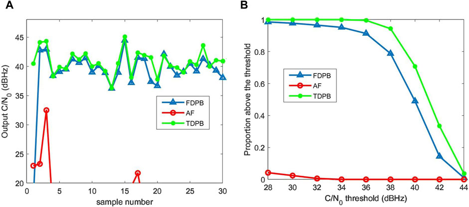
Figure 3. Comparison of pulse interference suppression performance. (A) C/N₀ results of the first 30 experiments. (B) Statistical results of C/N₀ of 500 experiments.

3.4.3 Chirp interference suppression performance

The sweep bandwidth of the chirp interference is randomly distributed between 4 and 20 MHz, and the sweep period is randomly distributed between 0.01 and 1 ms. The Monte Carlo experimental results are shown in Figure 4. At this time, statistically speaking, the TDPB algorithm has the worst performance. When the C/N₀ threshold is less than 42 dB Hz, the FDPB algorithm performs better than the AF algorithm, but when the C/N₀ threshold is greater than 42 dB Hz, the AF algorithm performs better than the FDPB algorithm.

Figure 4

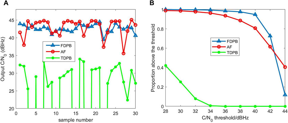
Figure 4. Comparison of chirp interference suppression performance. (A) C/N₀ results of the first 30 experiments. (B) Statistical results of C/N₀ of 500 experiments.

From the above analysis, it can be seen that for different types of interference, the optimal interference mitigation method in a statistical sense is different. For example, the AF algorithm has the best suppression performance for narrowband interference, and the TDPB algorithm has the best suppression performance for pulse interference. On the other hand, it is not difficult to see from Figures 1A, 2A, 3A that even for the same type of interference with different interference parameters, the optimal interference mitigation method is not the same.

4 IIM method

Considering that the interference environment faced by the receiver is unknown, dynamic, and uncertain, this paper proposes an IIM method, which automatically selects the optimal method to suppress interference based on the characteristics of interference, thereby improving the interference mitigation performance and robustness of the receiver.

4.1 Basic principles

The schematic diagram of the IIM method is shown in Figure 5. The input for IIM is the digital complex baseband signal received by the GNSS antenna and processed by signal conditioning (including amplification, frequency conversion, filtering, and sampling quantization). On one hand, the IIM processing performs three types of interference mitigation processing on the signal: FDPB, AF, and TDPB; On the other hand, it performs two-dimensional spectrum perception on the input signal. The deep learning network outputs the optimal method among the three anti-jamming processing based on the two-dimensional time-frequency spectrum and controls the switch to direct the output of the optimal anti-jamming method to signal acquisition, tracking, and PVT solution processing.

Figure 5

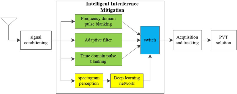
Figure 5. Block diagram of the IIM method.

Different types of interference or different parameters of the same interference will result in different time-frequency two-dimensional spectra, which means that the differences in interference types and parameters will be reflected in the time-frequency two-dimensional spectra. Therefore, a deep learning network can be constructed to automatically select the optimal interference mitigation method based on the time-frequency two-dimensional spectrum of the input signal. During the training stage, for each input sample, by traversing three interference mitigation methods, the corresponding output C/N₀ can be obtained. The interference mitigation method with the highest output C/N₀ is selected as the output (or label) of the deep learning network. After the network is trained, the network architecture and weights are fixed. During the deployment stage, the deep learning network automatically selects the optimal interference mitigation method based on the input interference type and parameters, and sends its interference mitigation output to subsequent processing through switch switching.

4.2 Implementation framework

4.2.1 Time frequency two-dimensional spectral sensing

The purpose of time-frequency two-dimensional spectrum sensing is to unfold the digital complex baseband signal after signal conditioning in the time-frequency two-dimensional plane. When there is interference, the unfolded time-frequency two-dimensional spectrum will reflect the type and parameters of interference.

This paper uses STFT to achieve time-frequency two-dimensional spectral sensing, and the process can be described by Equation 12 as follows [22]:

$S_x\left(j,k\right)={\left|{\displaystyle \sum _{n=0}^{N-1}}x\left(j\cdot P+n\right)w\left(n\right)e^{-j\frac{2\pi }{N}nk}\right|}^2(12)$

where $S_x\left(j,k\right)$ is a time-frequency two-dimensional spectral matrix, which is a non-negative real number. j and k are time serial number and frequency serial number respectively, $w\left(n\right)$ is a sliding window function with a length of N, which controls the data length and windowing type of each participation in Fourier transform, and P is the length of each sliding of the sliding window.

Figure 6 shows a sample of time-frequency two-dimensional spectra obtained for narrowband interference, pulse interference, and chirp interference. Each time-frequency image is in RGB format, with a size of 224 × 224 × 3.

Figure 6

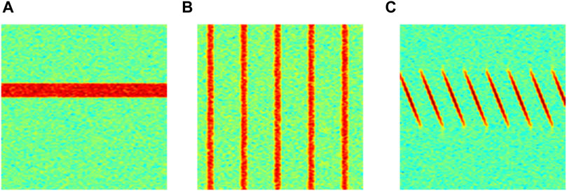
Figure 6. Time frequency two-dimensional spectra of different interference types. (A) Narrowband interference. (B) Pulse interference. (C) Chirp interference.

4.2.2 Deep learning network

Using pre-trained deep learning networks for optimal interference mitigation method selection, pre-trained network are deep learning networks that have been trained in millions of natural images and have good image feature extraction capabilities. When applied to the specialized field of GNSS IIM, only a small number of samples are needed to fine tune the pre trained network.

The selection of pre-training network should strike a balance between recognition performance (recognition accuracy) and resource consumption (recognition time). In this paper, GoogLeNet [23] is used as the pre-trained network model. GoogLeNet connects multiple well-designed Inception blocks in series with other layers (convolutional layer, fully connected layer) to form a 22-layer deep network. GoogLeNet was once one of the most effective models on ImageNet: it provides high recognition accuracy with low computational complexity.

5 Simulation analysis of IIM

Firstly, based on the simulation platform in Section 3, the Monte Carlo simulation method is used to generate sample data. The specific generation process is as follows: the signal received by the GNSS receiver is generated according to the signal model in Formula 1, and the global parameter settings are shown in Table 1. The parameters of the three types of interference are consistent with Section 3.4. 1,000 samples are generated under each interference, and a sample set containing 3,000 samples is generated in total. For each sample, by traversing three interference mitigation methods, one can obtain their respective output C/N₀. The interference mitigation method with the highest output C/N₀ is selected as the label for the sample.

Table 1

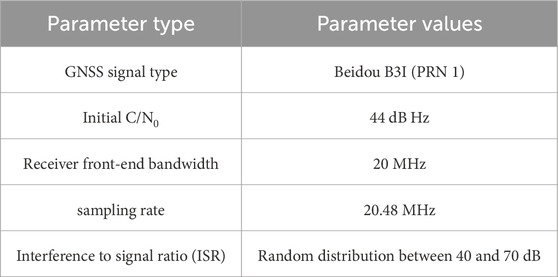
Table 1. Parameters used in simulation.

The entire sample set is divided into three parts: 2,400 samples are used as the training set (800 samples for each disturbance), 300 samples are used as the verification set (100 samples for each disturbance), and 300 samples are used as the test set (100 samples for each disturbance), so 80% of the whole sample is used for training, and 20% is used for verification and testing.

The experiment utilizes the PyTorch [24] deep learning framework to complete the model construction, training and testing. The hyperparameters of the neural network are set as follows: the optimizer selects Adam; the learning rate is set to 0.001; the batch size is set to 20; the maximum number of training epoch is set to 10; and the loss function is cross entropy loss.

Load the trained network model into the IIM method proposed in Section 4, validate it on the test set, and compare it with three traditional interference mitigation methods. The comparison results of interference mitigation performance are shown in Figure 7.

Figure 7

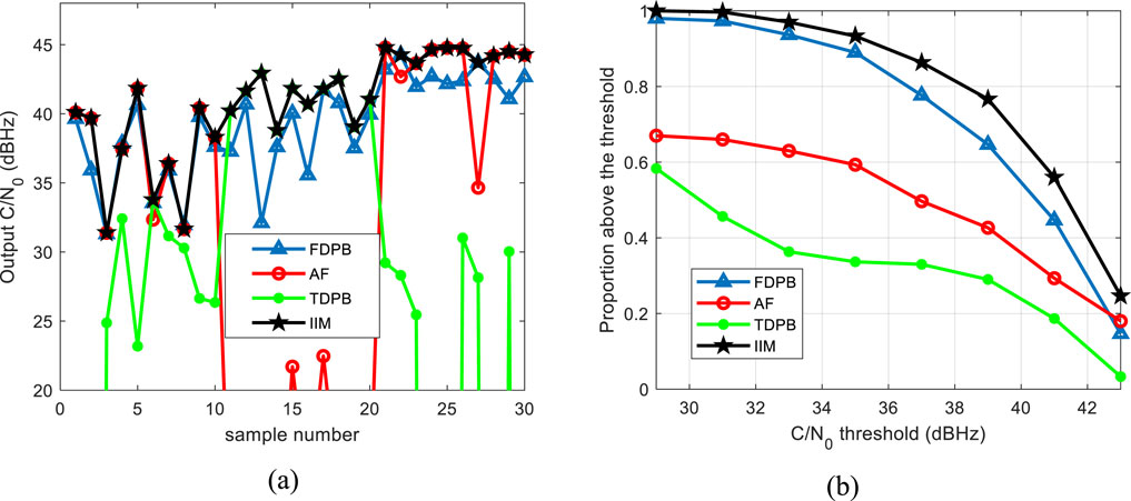
Figure 7. Comparison of interference suppression performance between proposed method and traditional methods. (A) C/N₀ results of the first 30 experiments. (B) Statistical results of C/N₀ on the entire test set.

Figure 7A shows the C/N₀ results obtained from the first 30 samples in the test set (including 10 narrowband interference, 10 pulse interference, and 10 chirp interference samples each). It can be seen that traditional interference mitigation methods have good suppression effects on one or two types of interference, but it is difficult to achieve good suppression effects on all three types of interference at the same time. However, the IIM method proposed in this paper can achieve this. Although the output C/N₀ obtained by the IIM method is not the highest on individual samples (because there is also a probability of errors in the prediction results of the network model), overall, the output C/N₀ obtained by it is the highest in most cases. Figure 7B shows the statistical results on the entire test set. It can be seen from the figure that the IIM method is the optimal interference mitigation method in a statistical sense, and the proportion of the C/N₀ above a given threshold (In engineering applications, it is generally agreed that the initial C/N₀ reduced by 3 dB is used as the threshold.) is more than 12% higher than traditional methods.

It should be particularly noted that, compared to traditional methods, IIM incorporates a spectrum sensing module and a deep learning network. The introduction of the deep learning network significantly increases the computational complexity by thousands of times. As a result, a dedicated GPU chip must be added specifically to accelerate the inference process of the deep learning model. Additionally, the inference process of the deep learning model introduces an extra processing latency of several milliseconds. The increase in computational complexity and processing latency limits the deployment of IIM in low-cost and real-time demanding GNSS receivers.

6 Open sky experiment

To further verify the proposed method, an open sky experiment is carried out. In this test, an antenna array based data collector is placed at a fixed position in the open wild for GNSS signal collection, while interfering signals are simulated and added in our SDR. This method is often used in GNSS jamming experiments [25, 26] to avoid impacting civil GNSS users. The open sky experiment configuration is shown in Figure 8.

Figure 8

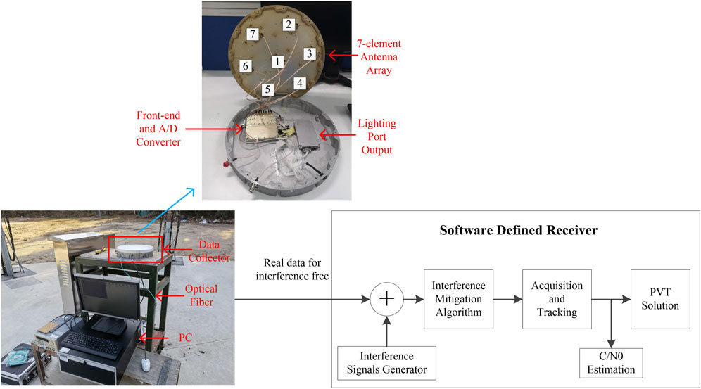
Figure 8. Open sky experiment configuration.

The data collector includes 7 antennas, a front-end, an A/D converter, and a lighting port output. It should be mentioned that only data from antenna 1 (i.e., the center antenna) is used in our experiment. The output baseband data (sampling frequency is 62/3 MHz and duration is 2,300 ms) of the data collector are stored on a personal computer (PC) and processed by the SDR.

For the SDR, firstly, interference signals are generated and added to the baseband data at 1,000 ms, the parameters of the three types of interference signals are consistent with Section 3.4. For each type of interference, 30 random samples are generated, totaling 90 samples. For each sample, the SDR is used for processing, and the performance of different interference mitigation methods is compared.

Figure 9 shows the processing results of the SDR for the B3I signal (PRN 1) under sweep chirp interference (ISR is 64.53 dB, sweep bandwidth is 16.27 MHz, and sweep period is 0.935 ms). It can be observed that before the interference is turned on (0–1000 ms), with direct pass-through processing, the output C/N₀ is around 43 dB Hz. After applying the IIM algorithm, the output C/N₀ is slightly lower than that of the direct pass-through processing, due to the insertion loss introduced by the interference mitigation processing. After the interference is turned on (1000 ms–2300 ms), the output C/N₀ of the direct pass-through processing drops rapidly, and the receiver loses track of the signal, while the output C/N₀ of the IIM algorithm remains essentially unchanged, allowing the receiver to maintain normal tracking of the signal, as seen in Figure 10.

Figure 9

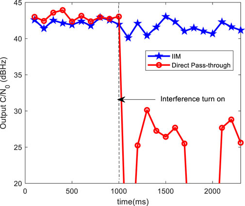
Figure 9. Output C/N₀ for IIM and direct pass-through.

Figure 10

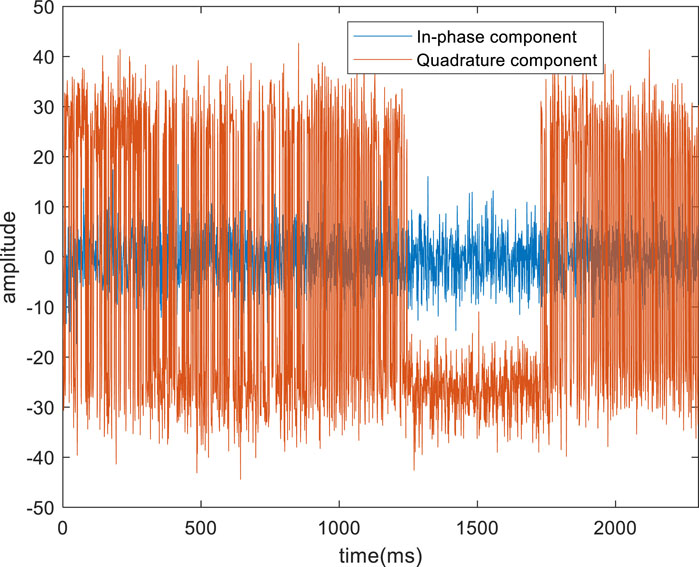
Figure 10. The in-phase and quadrature component of the prompt channel for IIM.

Figure 11 compares the time-frequency diagrams of the output signals obtained from direct pass-through and IIM. It can be seen that after applying IIM processing, the power of the chirp interference is significantly reduced, with a power level similar to that of the surrounding thermal noise, indicating that the IIM algorithm effectively suppresses the interference.

Figure 11

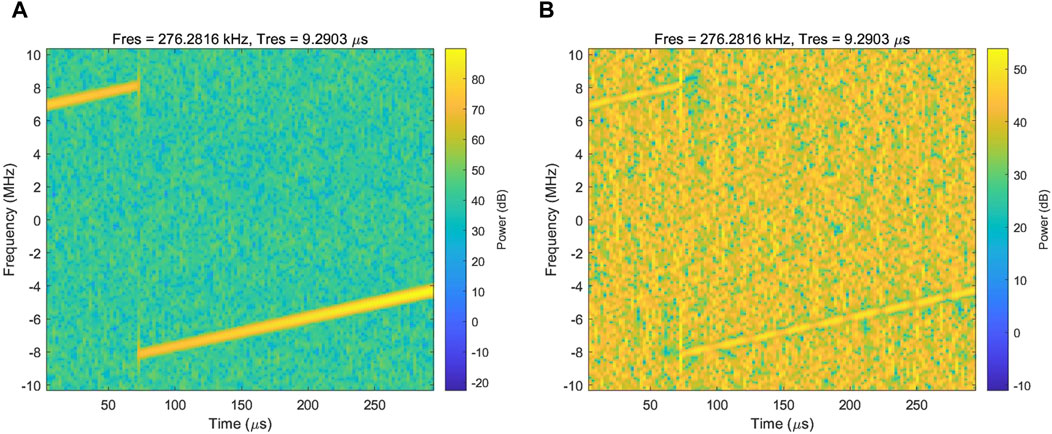
Figure 11. Interference mitigation performance for IIM. (A) Time-frequency diagrams of the output signals obtained from direct pass-through. (B) Time-frequency diagrams of the output signals obtained from IIM.

Finally, Figure 12 presents the statistical results across all 90 sample sets. For each sample, we take the average of the output C/N₀ results after the interference is turned on (with a duration of 1.3 s) as the final output C/N₀ result. It can be observed from the figure that the IIM method is statistically the optimal method, with its proportion above the threshold (initial C/N₀ minus 3 dB, i.e., 40 dB Hz) being more than 16% higher than that of traditional methods. This result is basically consistent with the outcomes derived from the simulation, with only minor differences in specific numerical values.

Figure 12

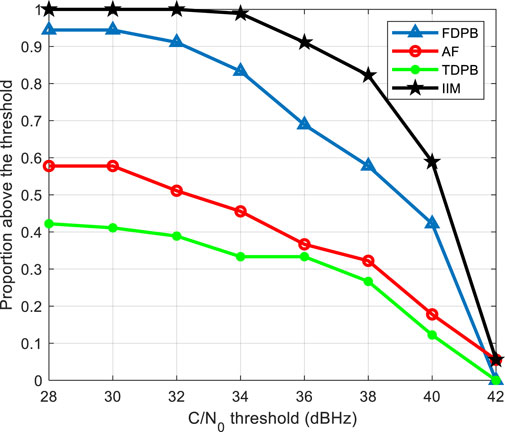
Figure 12. Comparison of interference mitigation performance.

7 Conclusion

This article examines the interference challenges encountered by GNSS receivers and introduces a deep learning-based approach for GNSS interference mitigation. The method begins by analyzing the input signal in a two-dimensional spectrogram and then employs a deep learning network to determine the optimal strategy among three interference mitigation algorithms. The selected optimal interference mitigation strategy is subsequently conveyed to the signal capture tracking and PVT calculation processes via a switching mechanism. Compared to traditional interference mitigation techniques, the method outlined in this paper is capable of adapting to various types of interference and different interference parameters, demonstrating effective suppression across a range of interference scenarios. Simulation and open-sky experimental results have confirmed the efficacy of this approach.

In conclusion, the proposed technique is a potent interference mitigation tool that can substantially broaden the operational range of GNSS receivers under interference conditions. Future enhancements could focus on reducing computational complexity and enhancing performance in scenarios with multiple concurrent interference signals.

Data availability statement

The raw data supporting the conclusions of this article will be made available by the authors, without undue reservation.

Author contributions

FC: Writing–original draft. ZL: Writing–review and editing. LH: Writing–review and editing. YX: Writing–review and editing. BR: Writing–review and editing. QZ: Writing–review and editing.

Funding

The author(s) declare that financial support was received for the research, authorship, and/or publication of this article. This research was supported in part by the Natural Science Foundation of China (NSFC), grants No. 62303475 and U20A20193.

Acknowledgments

The authors would like to thank the editors and reviewers for their efforts in supporting the publication of this paper.

Conflict of interest

The authors declare that the research was conducted in the absence of any commercial or financial relationships that could be construed as a potential conflict of interest.

Generative AI statement

The author(s) declare that no Generative AI was used in the creation of this manuscript.

Publisher’s note

All claims expressed in this article are solely those of the authors and do not necessarily represent those of their affiliated organizations, or those of the publisher, the editors and the reviewers. Any product that may be evaluated in this article, or claim that may be made by its manufacturer, is not guaranteed or endorsed by the publisher.

References

1. Ren B, Chen F, Ni S, Han C, Lu Z, Han S. Performance analysis of repeater spoofing suppression based on GNSS multi-beam receiver. Front Phys (2022) 10:970132. doi:10.3389/fphy.2022.970132

CrossRef Full Text | Google Scholar

2. Ni S, Binbin R, Chen F, Lu Z, Wang J, Ma P, et al. GNSS spoofing suppression based on multi-satellite and multi-channel array processing. Front Phys (2022) 10:905918. doi:10.3389/fphy.2022.905918

CrossRef Full Text | Google Scholar

3. Chen F. GNSS antenna array receiver interference suppression and measurement deviation compensation technology. Changsha: National University of Defense Technology (2017).

Google Scholar

4. Gao GX, Sgammini M, Lu M, Kubo N. Protecting GNSS receivers from jamming and interference. Proc IEEE (2016) 104(6):1327–38. doi:10.1109/JPROC.2016.2525938

CrossRef Full Text | Google Scholar

5. Morales Ferre R, de la Fuente A, Lohan ES. Jammer classification in GNSS bands via machine learning algorithms. Sensors (2019) 19(22):4841. doi:10.3390/s19224841

PubMed Abstract | CrossRef Full Text | Google Scholar

6. Morales Ferre R, Richter P, Falletti E, Fuente ADL, Lohan ES. A survey on coping with integral interference in satellite navigation for manned and unmanned aerial. IEEE Commun Surveys&Tutorials (2020) 22(1):249–91. doi:10.1109/COMST.2019.2949178

CrossRef Full Text | Google Scholar

7. Wang P, Cetin E, Dempster A, Wang Y, Wu S. GNSS interference detection using statistical analysis in the time frequency domain. IEEE Trans Areospace Electron Syst (2018) 54(1):416–28. doi:10.1109/TAES.2017.2760658

CrossRef Full Text | Google Scholar

8. Kaplan ED, Yanhong K. Principles and applications of GPS. 2nd ed. Beijing: Electronic Industry Press (2007).

Google Scholar

9. Borio D, Gioia C. GNSS interference mitigation: a measurement and position domain assessment. NAVIGATION: J Inst Navigation (2021) 68(1):93–114. doi:10.1002/navi.391

CrossRef Full Text | Google Scholar

10. Borio D, Camorano L, Presti LL. Two pole and multi pole notch filters: a computationally effective solution for GNSS interference de-tection and mitigation. IEEE Syst J (2008) 2(1):38–47. doi:10.1109/JSYST.2007.914780

CrossRef Full Text | Google Scholar

11. Song J, Lu Z, Xiao Z, Li B, Sun G. Optimal order of time domain adaptive filter for anti jamming navigation receiver. Remote Sensing (2021) 14(1):48. doi:10.3390/rs14010048

CrossRef Full Text | Google Scholar

12. Fan G, Huang Y, Su Y, Li J, Sun G. A reduced bias delay lock loop for adap-tive filters. Advancements Space Res (2017) 59(1):230–5. doi:10.1016/j.asr.2016.09.007

CrossRef Full Text | Google Scholar

13. Huo S, Nie J, Wang F. Block flow noise power estimation algorithm for pulse interference detection of GNSS receivers. Electronics Lett (2015) 51(19):1522–4. doi:10.1049/el.2015.1445

CrossRef Full Text | Google Scholar

14. Danielle B, Pau C. Complex signal non linearity for robust GNSS interference mitigation. IET Radar, Sonar&Navigation (2018) 12(8):900–9. doi:10.1049/iet-rsn.2017.0552

CrossRef Full Text | Google Scholar

15. Chen F, Liu Z, Huang L, Lu Z. Low complexity suppression method for fast sweep interference in satellite navigation receivers. J Natl Univ Defense Technology (2023) 45(5):105–10. doi:10.11887/j.cn.202305012

CrossRef Full Text | Google Scholar

16. Borio D. Swept GNSS jamming mitigation through pulse Blanking. In: 2016 European navigation conference (ENC). IEEE (2016). p. 1–8. doi:10.1109/EURONAV.2016.7530549

CrossRef Full Text | Google Scholar

17. Akeret J, Chang C, Lucchi A, Refregier A. Radio Frequency Interference mitigation using deep convolutional neural networks. Astron Comput (2016) 18:35–9. doi:10.1016/j.ascom.2017.01.002

CrossRef Full Text | Google Scholar

18. Alireza VS, Bassett BA, Nadeem O, Yabebal F, Chris F. Deep learning improves identification of radio frequency interference. Monthly Notices R Astronomical Soc (2020)(1) 1. doi:10.1093/mnras/staa2724

CrossRef Full Text | Google Scholar

19. Haomin S, Hui D, Feng W, Ying M, Tingting X, Oleg S, et al. A robust RFI identification for radio interferometry based on a convolutional neural network. Monthly Notices R Astronomical Soc (2022)(2) 2. doi:10.1093/mnras/stac570

CrossRef Full Text | Google Scholar

20. Kennedy F, Bull P, Wilensky MJ, Burba J, Choudhuri S. Statistical recovery of 21 cm visibilities and their power spectra with Gaussian-constrained realizations and gibbs sampling. IOP Publishing Ltd (2023). doi:10.3847/1538-4365/acc324

CrossRef Full Text | Google Scholar

21. Leeney SAK, Handley WJ, Acedo EDL. Bayesian approach to radio frequency interference mitigation. Phys Rev (2023) 108(6 Pt.A):062006. doi:10.1103/physrevd.108.062006

CrossRef Full Text | Google Scholar

22. Ouyang X, Amin MG. Short-time fourier transform receiver for nonstationary interference excision in direct sequence spread spectrum communications. IEEE Trans Signal Process (2001) 49:851–63. doi:10.1109/78.912929

CrossRef Full Text | Google Scholar

23. Szegedy C, Liu W, Jia Y, Sermanet P, Reed S, Anguelov D, et al. Going deeper with convolutions. In: Proceedings of the IEEE conference on computer vision and pattern recognition (2015). USA. 18-20 June 1996. p. 1–9.

Google Scholar

24. Paszke A, Lerer A, Killeen T, Antiga L, Yang E, Tejani A, et al. PyTorch: an imperative style, high-performance deep learning library. In: Advances in neural information processing systems 32, volume 11 of 20: 32nd conference on neural information processing systems (NeurIPS 2019). (2020) Vancouver (CA), December 8-14, 2019.

Google Scholar

25. Xie Y, Chen F, Huang L, Liu Z, Wang F. Carrier phase bias correction for GNSS space-time array processing using time-delay data. GPS Solutions (2023) 27(3):113. doi:10.1007/s10291-023-01456-y

CrossRef Full Text | Google Scholar

26. Mosavi MR, Rezaei MJ, Pashaian M, Moghaddasi MS. A fast and accurate anti-jamming system based on wavelet packet transform for GPS receivers. GPS solutions (2017) 21:415–26. doi:10.1007/s10291-016-0535-z

CrossRef Full Text | Google Scholar