Some novel exact solutions for the generalized time-space fractional coupled Hirota-Satsuma KdV equation

In this paper, two efficient methods, namely the modified $\left(G^{\prime }/G,1/G\right)$-expansion method and the ${\mathit{G}}^{\prime }/\left(b{G}^{\prime }+G+a\right)$-expansion method, are employed to obtain novel exact wave solutions for the generalized time-space fractional coupled Hirota-Satsuma KdV equation. Various types of analytical explicit solutions, including well-known bell-shape solitons, mixed solitary wave solutions, and periodic wave solutions are obtained. These solutions are of great significance for revealing the nonlinear interaction between two long waves with different dispersion effects. The two-dimensional and three-dimensional distribution maps and contour plots corresponding to partial solutions are simulated to visually display the evolution process of relevant physical quantities over time. Moreover, the potential applications of these solutions in nano/micro devices and systems, especially in MEMS (Micro-Electro-Mechanical Systems) are discussed. It is demonstrated that the methods and processes utilized have strong applicability for constructing analytical solutions of nonlinear evolution equations.

1 Introduction

As we all know, nonlinear partial differential equation models are applied to almost every corner of social life. For example, various nonlinear soliton equations can be used to describe wave phenomena in many natural sciences and engineering fields such as fluid physics, solid state physics, laser physics, astrophysics, geophysics, lattice vibration, optical fiber communication, quantum mechanics, geomechanics, oceanography, superconductivity, field theory, transportation, etc. Since fractional order nonlinear systems can describe these nonlinear processes more accurately than integer order systems, studying the solution of fractional order nonlinear systems is particularly important in the development of natural sciences, and has always been a hot topic for domestic and foreign scholars. Till now, people have given many forms of fractional derivative definitions for different situations. For example, Riemann-Liouville definition [1], Caputo definition [2], Jumaries’s definition [3], Atangana’s definition [4], Atangana-Baleanu-Riemann definition [5], conformable definition [6], Abu-Shady-Kaabar definition [7], He’s definition [8], etc. [9–15]. Each definition has its own advantages and disadvantages, for example, the Riemann-Liouville definition is to consider the derivative of the integral factor, the Caputo definition is to consider the integration of the derivative factor, the Jumaries’s definition is to consider the influence of the initial value and the He’s definition takes into account the more general problem of initial values, etc., and their efficiency varies in the process of solving some specific problems. In order to find the analytical solutions of nonlinear fractional partial differential equations, many domestic and foreign scholars have made great efforts, and the existing methods mainly include the Bäcklund transformation method [16], the homogeneous equilibrium method [17], the Riccati equation expansion method [18], the F-expansion method [19], the Jacobi elliptic function expansion method [20], the generalized expansion method [21], the Darboux transform method [22], the Lie symmetry method [23], the Adomian decomposition method [24], The homotopy perturbation method [25], the variational iterative method [26], and so on [27–29]. These methods have their own advantages and characteristics, providing powerful tools for exploring the solutions of complex nonlinear equations.

Furthermore, the applications of these solutions are not limited to traditional fields. In the era of rapid development of nano/micro technology, they have potential applications in nano/micro devices and systems, especially in MEMS (Micro-Electro-Mechanical Systems) [30]. MEMS technology combines mechanical elements, sensors, actuators, and electronics on a microscale, and understanding the behavior of fractional partial differential equations can contribute to the design, optimization, and performance improvement of MEMS devices [31]. For example, in the field of sensors, fractional order models can help analyze and predict the response of micro-sensors to various stimuli more accurately. In actuators, the solutions of fractional equations can provide insights into the dynamic behavior and control strategies [32]. Additionally, in integrated micro-systems, the understanding of fractional order phenomena can enhance the functionality and reliability of the overall system [33, 34].

The study of fractional order nonlinear partial differential equations and their solutions is not only of theoretical significance but also has practical applications in a wide range of fields, especially in the emerging field of nano/micro devices and systems such as MEMS. Our research is based on the definition of M-fractional derivative proposed by Sousa and Oliveira recently [35], this new fractional derivative definition generalizes the conformable derivative by a truncated Mittag-Leffler function of one parameter [6]. By adopting the ideas of generalized Jacobi elliptic function method [36], modified $\left(G^{\prime }/G,1/G\right)$-expansion method [38, 39] and $G^{\prime }/\left(b{G}^{\prime }+G+a\right)$-expansion method [40], using the homogeneous equilibrium principle [41] and mathematical symbolic calculation software, to study a class of generalized time-space fractional coupled Hirota-Satsuma KdV system arising in interaction of two long waves with different dispersion effects under the definition of M-fractional derivative,

$\left\{\begin{array}{l}{u}_t^{\alpha }=\frac{1}{4}{u}_{xxx}^{3\beta }+3u{u}_x^{\beta }+3{\left(-v^2+w\right)}_x^{\beta },\\ v_t^{\alpha }=-\frac{1}{2}{v}_{xxx}^{3\beta }-3u{v}_x^{\beta },\\ w_t^{\alpha }=-\frac{1}{2}{w}_{xxx}^{3\beta }-3u{w}_x^{\beta },0<\alpha ,\beta \le 1.\end{array}\right.(1)$

where ${\left(\cdot \right)}_t^{\alpha }=D_{M,t}^{{\gamma }_1,\alpha }\left(\cdot \right),{\left(\cdot \right)}_x^{\beta }=D_{M,x}^{{\gamma }_2,\beta }\left(\cdot \right),{\left(\cdot \right)}_{xxx}^{3\beta }=D_{M,x}^{{\gamma }_2,\beta }\left(D_{M,x}^{{\gamma }_2,\beta }\left(D_{M,x}^{{\gamma }_2,\beta }\left(\cdot \right)\right)\right)$ mean the M-fractional derivative [35, 39, 42, 43], $u=u\left(x,t\right),v=v\left(x,t\right),w=w\left(x,t\right).$ If we select $\alpha =1,\beta =1$, we get the well-known integer order coupled Hirota-Satsuma KdV equation. The equation is mainly used to describe the interaction between two columns of long waves with different dispersion relations [44]. Ref. [45] studies the case when $w=0$, and Ref. [46] obtains the general form when $w\ne 0$ through a matrix spectrum problem. Ref. [47] studies its elliptic sine function solution by direct expansion method. Refs. [48, 49] use the modified Riccati expansion method and the extended elliptic function expansion method to study its exact solutions in various forms. Ref. [50] studies the Darboux transformation of the equation, and the branch structure of the equation is studied by the theory of plane dynamic system in reference [51]. Under the definition of conformable fractional derivative with $\beta =1$, Ref. [52] studies the analytical solutions of system (1) by using auxiliary equation method and series expansion method, and Ref. [53] uses $\left(G^{\prime }/G\right)$ expansion method to study the solitary wave solution and trigonometric function periodic solution of system (1). Additional relevant studies on the system can be referred to Refs. [54–58]. Let’s first introduce several relevant definitions and properties.

Definition 1. For a function $f\left(t\right):[0,\infty )\to R$, We defined the M-fractional derivative operator of $f\left(t\right)$ of order $\alpha$ as [35].

$D_{M,t}^{\gamma ,\alpha }f\left(t\right)=\underset{\epsilon \to 0}{\lim }\frac{f\left(t{E}_{\gamma }\left(\epsilon t^{-\alpha }\right)\right)-f\left(t\right)}{\epsilon },\gamma \ge 0,0<\alpha \le 1.(2)$

where $E_{\gamma }\left(t\right)={\displaystyle \sum _{k=0}^{\infty }}\frac{t^k}{\mathrm{\Gamma }\left(\gamma k+1\right)}$ is a Mittag-Leffler function of parameter $\gamma$.

Property 1. The M-fractional derivative operator of $f\left(t\right)$ of order $\alpha$ have the following important properties [35, 39, 42, 43]:

(1) $D_{M,t}^{\gamma ,\alpha }f\left(t\right)=\frac{t^{-\alpha }}{\mathrm{\Gamma }\left(\gamma +1\right)}\frac{df\left(t\right)}{dt}.$

(2) $D_{M,t}^{\gamma ,\alpha }\left(af\left(t\right)+bg\left(t\right)\right)=a{D}_{M,t}^{\gamma ,\alpha }f\left(t\right)+b{D}_{M,t}^{\gamma ,\alpha }g\left(t\right),\forall a,b\in R.$

(3) $D_{M,t}^{\gamma ,\alpha }\left(f\left(t\right)g\left(t\right)\right)=f\left(t\right)D_{M,t}^{\gamma ,\alpha }g\left(t\right)+g\left(t\right)D_{M,t}^{\gamma ,\alpha }f\left(t\right).$

(4) $D_{M,t}^{\gamma ,\alpha }\left(f\left(t\right)/g\left(t\right)\right)=\left[g\left(t\right)D_{M,t}^{\gamma ,\alpha }f\left(t\right)-f\left(t\right)D_{M,t}^{\gamma ,\alpha }g\left(t\right)\right]/g^2\left(t\right).$

(5) $D_{M,t}^{\gamma ,\alpha }\left(f\circ g\right)\left(t\right)=f^{\prime }\left(g\left(t\right)\right)D_{M,t}^{\gamma ,\alpha }g\left(t\right)=\frac{t^{-\alpha }}{\mathrm{\Gamma }\left(\gamma +1\right)}{f}^{\prime }\left(g\left(t\right)\right)\frac{dg\left(t\right)}{dt}.$

Definition 2. The M-fractional derivative system (1) determined by Definition 1 and Equation 2 performs the following travelling wave transformation:

$u=u\left(x,t\right)=u\left(\xi \right),v=v\left(x,t\right)=v\left(\xi \right),w=w\left(x,t\right)=w\left(\xi \right)(3)$

$\xi =\frac{\mathrm{\Gamma }\left({\gamma }_2+1\right)}{\beta }2kx+\frac{\mathrm{\Gamma }\left({\gamma }_1+1\right)}{\alpha }C{t}^{\alpha }+{\xi }_0,{\gamma }_1,{\gamma }_2\ge 0,0<\alpha ,\beta \le 1(4)$

where $k,C$ are undetermined constants, ${\gamma }_1,{\gamma }_2{\xi }_0$ are arbitrary constants.

Substituting Equations 3, 4 into Equation 1, we obtain the following system of ordinary differential equations:

$\left\{\begin{array}{l}C{u}^{\prime }=2k^3{u}^{‴}+6ku{u}^{\prime }-12kv{v}^{\prime }+6k{w}^{\prime },\\ C{v}^{\prime }=-4k^3{v}^{‴}-6ku{v}^{\prime },\\ C{w}^{\prime }=-4k^3{w}^{‴}-6ku{w}^{\prime }.\end{array}\right.(5)$

where

$u^{\prime }=\frac{du}{d\xi },u^{‴}=\frac{d^{3}u}{d{\xi }^3},v^{\prime }=\frac{dv}{d\xi },v^{‴}=\frac{d^{3}v}{d{\xi }^3},w^{\prime }=\frac{dw}{d\xi },w^{‴}=\frac{d^{3}w}{d{\xi }^3}.$

2 Description of the two methods

2.1 The modified $\left(G^{\prime }/G,1/G\right)$-expansion method

Consider the following nonlinear M-fractional nonlinear partial differential equations:

$\left\{\begin{array}{l}{E}_1\left(u,u_t^{\alpha },u_x^{\beta },u{u}_x^{\beta },v,v_t^{\alpha },v_x^{\beta },v{v}_x^{\beta },w,w_t^{\alpha },w_x^{\beta },w{w}_x^{\beta },u{v}_x^{\beta },u{w}_x^{\beta },v{w}_x^{\beta },\cdots \right)=0,\\ E_2\left(u,u_t^{\alpha },u_x^{\beta },u{u}_x^{\beta },v,v_t^{\alpha },v_x^{\beta },v{v}_x^{\beta },w,w_t^{\alpha },w_x^{\beta },w{w}_x^{\beta },u{v}_x^{\beta },u{w}_x^{\beta },v{w}_x^{\beta },\cdots \right)=0,\\ E_3\left(u,u_t^{\alpha },u_x^{\beta },u{u}_x^{\beta },v,v_t^{\alpha },v_x^{\beta },v{v}_x^{\beta },w,w_t^{\alpha },w_x^{\beta },w{w}_x^{\beta },u{v}_x^{\beta },u{w}_x^{\beta },v{w}_x^{\beta },\cdots \right)=0.\end{array}\right.(6)$

By using the wave transformation (4), Equation 6 is converted into a nonlinear ordinary differential equations (ODE):

$\left\{\begin{array}{l}{O}_1\left(u,u^{\prime },u{u}^{\prime },v,v^{\prime },v{v}^{\prime },w,w^{\prime },w{w}^{\prime },u{v}^{\prime },u{w}^{\prime },v{w}^{\prime },\cdots \right)=0,\\ O_2\left(u,u^{\prime },u{u}^{\prime },v,v^{\prime },v{v}^{\prime },w,w^{\prime },w{w}^{\prime },u{v}^{\prime },u{w}^{\prime },v{w}^{\prime },\cdots \right)=0,\\ O_3\left(u,u^{\prime },u{u}^{\prime },v,v^{\prime },v{v}^{\prime },w,w^{\prime },w{w}^{\prime },u{v}^{\prime },u{w}^{\prime },v{w}^{\prime },\cdots \right)=0.\end{array}\right.(7)$

Assume that Equation 7 has the following solution:

$\left\{\begin{array}{l}u={\displaystyle \sum _{i=0}^M}{a}_i{\psi }^i+{\displaystyle \sum _{j=1}^M}{b}_j{\varphi }^j+{\displaystyle \sum _{i=1}^{M-1}}{c}_i{\psi }^i\varphi ,\\ v={\displaystyle \sum _{i=0}^N}{d}_i{\psi }^i+{\displaystyle \sum _{j=1}^N}{e}_j{\varphi }^j+{\displaystyle \sum _{i=1}^{N-1}}{f}_i{\psi }^i\varphi ,\\ w={\displaystyle \sum _{i=0}^P}{g}_i{\psi }^i+{\displaystyle \sum _{j=1}^P}{h}_j{\varphi }^j+{\displaystyle \sum _{i=1}^{P-1}}{l}_i{\psi }^i\varphi .\end{array}\right.(8)$

where $M,N,P$ are balance numbers, $\varphi =\varphi \left(\xi \right)=\frac{G^{\prime }}{G},\psi =\psi \left(\xi \right)=\frac{1}{G}$, $a_i,b_j,c_i,d_i,e_j,f_i,g_i,h_j,l_i$ and variable function $\xi =\xi \left(x,t\right)$ are determined later. The $G$ is a solution of the following auxiliary ODE:

$G^{″}=\epsilon G-\epsilon \mu .(9)$

where $\epsilon =\pm 1,\mu$ is an arbitrary real number. It satisfies the following constrained conditions:

${\varphi }^{\prime }=\epsilon -\epsilon \mu \psi -{\varphi }^2,{\psi }^{\prime }=-\varphi \psi ,{\varphi }^2=\epsilon -2\epsilon \mu \psi -\epsilon \left(b^2-\epsilon c^2-{\mu }^2\right){\psi }^2.(10)$

where arbitrary constants $\mu ,b,c$ satisfied the relation $c^2+b^2+{\mu }^2\ne 0.$ Equations 9, 10 admit the following solutions

Case 1: When $\epsilon =1$, we have $G=b\cosh \xi +c\sinh \xi +\mu$, thus

$\varphi =\frac{G^{\prime }}{G}=\frac{b\sinh \xi +c\cosh \xi }{b\cosh \xi +c\sinh \xi +\mu },\psi =\frac{1}{G}=\frac{1}{b\cosh \xi +c\sinh \xi +\mu }.(11)$

Case 2: When $\epsilon =-1$, we have $G=b\cos \xi +c\sin \xi +\mu$, thus

$\varphi =\frac{G^{\prime }}{G}=\frac{-b\sin \xi +c\cos \xi }{b\cos \xi +c\sin \xi +\mu },\psi =\frac{1}{G}=\frac{1}{b\cos \xi +c\sin \xi +\mu }.(12)$

Substituting Equations 8, 10 into Equation 7 and setting coefficients of ${\varphi }^i{\psi }^j\left(i=0,1,j=0,1,2,3,4,\cdots \right)$ to zero yield a set of algebraic equations (AEs) for $a_i,b_j,c_i,d_i,e_j,f_i,g_i,h_j,l_i,b,c,\mu ,k,C$. After solving the AEs and substituting each of the solutions $\varphi \left(\xi \right),\psi \left(\xi \right)$ from Equations 11, 12 along with (4) into Equation 1, we can get the analytical solutions of Equation 1.

Remark 1. Due to the arbitrariness of taking values of $b,c,\mu$, this method can encompass a lot of other methods, for example, when $\mu =0$, it includes the results of (G$\prime$/G) method and generalized (G$\prime$/G)-expansion method in Refs. [59, 60], if selecting special values of $b,c,\mu$, we can easily obtain all results of the Riccati equation method generalized in literature and the Kudryashov method generalized in Refs. [48, 61, 62]. Therefore, the method is highly applicable.

2.2 The $G^{\prime }/\left(b{G}^{\prime }+G+a\right)$-expansion method

Assume that Equation 7 has the following solution

$\left\{\begin{array}{l}u={\displaystyle \sum _{i=0}^M}{a}_i{\left(\frac{G^{\prime }}{b{G}^{\prime }+G+a}\right)}^i,\\ v={\displaystyle \sum _{i=0}^N}{b}_i{\left(\frac{G^{\prime }}{b{G}^{\prime }+G+a}\right)}^i,\\ w={\displaystyle \sum _{i=0}^P}{c}_i{\left(\frac{G^{\prime }}{b{G}^{\prime }+G+a}\right)}^i.\end{array}\right.(13)$

where $M,N,P$ are balance numbers. Parameters $a_i,b_i,c_i$ are determined later. $G=G\left(\xi \right)$ satisfies the following second-order ordinary differential equation:

$G^{″}=-\frac{\lambda }{b}{G}^{\prime }-\frac{\mu }{b^2}G-\frac{\mu }{b^2}a(14)$

Set $F=\frac{G^{\prime }}{b{G}^{\prime }+G+a}$, then $F$ satisfies

$F^{\prime }=\left(\lambda -\mu -1\right)F^2+\frac{1}{b}\left(2\mu -\lambda \right)F-\frac{1}{b^2}\mu (15)$

Equations 14, 15 admit the following solutions.

Case 1: When $\Delta ={\lambda }^2-4\mu >0$, we have the solitary wave solution

$G=-a+C_1{e}^{\frac{1}{2b}\left(-\lambda -\sqrt{\Delta }\right)\xi }+C_2{e}^{\frac{1}{2b}\left(-\lambda +\sqrt{\Delta }\right)\xi }(16)$

$F=\frac{C_1\left(\lambda +\sqrt{\Delta }\right)+C_2\left(\lambda -\sqrt{\Delta }\right)e^{\frac{\sqrt{\Delta }}{b}\xi }}{b{C}_1\left(\lambda -2+\sqrt{\Delta }\right)+b{C}_2\left(\lambda -2-\sqrt{\Delta }\right)e^{\frac{\sqrt{\Delta }}{b}\xi }}(17)$

Case 2: When $\Delta ={\lambda }^2-4\mu <0$, we have the periodic wave solution

$G=e^{-\frac{\lambda }{2b}\xi }\left(C_1\cos \left(\frac{\sqrt{-\Delta }}{2b}\xi \right)+C_2\sin \left(\frac{\sqrt{-\Delta }}{2b}\xi \right)\right)-a(18)$

$F=\frac{\left(\lambda C_1-\sqrt{-\Delta }{C}_2\right)\cos \left(\frac{\sqrt{-\Delta }}{2b}\xi \right)+\left(\lambda C_2+\sqrt{-\Delta }{C}_1\right)\sin \left(\frac{\sqrt{-\Delta }}{2b}\xi \right)}{b\left(\left(\lambda -2\right)C_1-\sqrt{-\Delta }{C}_2\right)\cos \left(\frac{\sqrt{-\Delta }}{2b}\xi \right)+b\left(\left(\lambda -2\right)C_2+\sqrt{-\Delta }{C}_1\right)\sin \left(\frac{\sqrt{-\Delta }}{2b}\xi \right)}(19)$

Case 3: When $\Delta ={\lambda }^2-4\mu =0$, we have the rational function solution

$G=C_1{e}^{-\frac{\lambda }{2b}\xi }+C_2\xi e^{-\frac{\lambda }{2b}\xi }-a(20)$

$F=\frac{2b{C}_2-\lambda C_1-\lambda C_2\xi }{2b^2{C}_2+b\left(2-\lambda \right)\left(C_1+C_2\right)\xi }(21)$

Substituting Equations 13, 15 into Equation 7 and setting coefficients of $F^i\left(i=0,1,2,3,4,\cdots \right)$ zero yield a set of AEs for $a_i,b_i,c_i,b,\lambda ,\mu ,k,C$, after solving the AEs with the aid of mathematical software, the wave solutions of Equation 1 can be obtained by these solutions and Equations 4, 16–21.

3 Exact solutions to the Hirota-Satsuma KdV equation

3.1 Solving Eq. (1) by the modified $\left(G^{\prime }/G,1/G\right)$-expansion method

From the homogeneous equilibrium principle [41], we can get $M=2,N=2,P=2$ in Equation 8. We assume that Equation 5 has solutions in the following form

$\left\{\begin{array}{l}u=a_0+a_1\psi +a_2{\psi }^2+a_3\varphi +a_4\psi \varphi +a_5{\varphi }^2,\\ v=b_0+b_1\psi +b_2{\psi }^2+b_3\varphi +b_4\psi \varphi +b_5{\varphi }^2,\\ w=c_0+c_1\psi +c_2{\psi }^2+c_3\varphi +c_4\psi \varphi +c_5{\varphi }^2.\end{array}\right.(22)$

where $a_i,b_i,c_i\left(i=0,\cdots ,5\right)$ are undetermined constants.

Substituting Equations 22, 10 into Equation 5, and setting the coefficients of ${\varphi }^i{\psi }^j(i=0,1,$$\left.j=0,1,2,3,4,\cdots \right)$ to zero yield a set of algebraic equations (AEs) for $a_i,b_i,c_i,b,c,\mu ,k,C$.

$\begin{array}{l}\psi :C\epsilon \mu a_3-2k^3{\epsilon }^2\mu a_3-6k\epsilon \mu a_0{a}_3+6k\epsilon a_1{a}_3-Cϵa_4+2k^3{\epsilon }^2{a}_4+6k\epsilon a_0{a}_4-18k{\epsilon }^2\mu a_3{a}_5+6k{\epsilon }^2{a}_4{a}_5+12k\epsilon \mu b_0{b}_3\\ -12k\epsilon b_1{b}_3-12k\epsilon b_0{b}_4+36k{\epsilon }^2\mu b_3{b}_5-12k{\epsilon }^2{b}_4{b}_5-6k\epsilon \mu c_3+6k\epsilon c_4=0,\\ \varphi \psi :-C{a}_1+2k^3\epsilon a_1+6k{a}_0{a}_1-6k\epsilon \mu a_3^2+6k\epsilon a_3{a}_4+2C\epsilon \mu a_5-4k^3{\epsilon }^2\mu a_5-12k\epsilon \mu a_0{a}_5+6k\epsilon a_1{a}_5-12k{\epsilon }^2\mu a_5^2\\ -12k{b}_0{b}_1+12k\epsilon \mu b_3^2-12k\epsilon b_3{b}_4+24k\epsilon \mu b_0{b}_5-12k\epsilon b_1{b}_5+24k{\epsilon }^2\mu b_5^2+6k{c}_1-12k\epsilon \mu c_5=0,\\ {\psi }^2:b^{2}C\epsilon a_3-c^{2}C{\epsilon }^2{a}_3-8b^2{k}^3{\epsilon }^2{a}_3+8c^2{k}^3{\epsilon }^3{a}_3-C\epsilon {\mu }^2{a}_3+14k^3{\epsilon }^2{\mu }^2{a}_3-6b^{2}k\epsilon a_0{a}_3+6c^{2}k{\epsilon }^2{a}_0{a}_3+6k\epsilon {\mu }^2{a}_0{a}_3\\ -18k\epsilon \mu a_1{a}_3+12k\epsilon a_2{a}_3+3C\epsilon \mu a_4-30k^3{\epsilon }^2\mu a_4-18k\epsilon \mu a_0{a}_4+12k\epsilon a_1{a}_4-18b^{2}k{\epsilon }^2{a}_3{a}_5+18c^{2}k{\epsilon }^3{a}_3{a}_5+54k{\epsilon }^2{\mu }^2{a}_3{a}_5\\ -42k{\epsilon }^2\mu a_4{a}_5+12b^{2}k\epsilon b_0{b}_3-12c^{2}k{\epsilon }^2{b}_0{b}_3-12k\epsilon {\mu }^2{b}_0{b}_3+36k\epsilon \mu b_1{b}_3-24k\epsilon b_2{b}_3+36k\epsilon \mu b_0{b}_4-24k\epsilon b_1{b}_4+36b^{2}k{\epsilon }^2{b}_3{b}_5\\ -36c^{2}k{\epsilon }^3{b}_3{b}_5-108k{\epsilon }^2{\mu }^2{b}_3{b}_5+84k{\epsilon }^2\mu b_4{b}_5-6b^{2}k\epsilon c_3+6c^{2}k{\epsilon }^2{c}_3+6k\epsilon {\mu }^2{c}_3-18k\epsilon \mu c_4=0,\\ \varphi {\psi }^2:-12k^3\epsilon \mu a_1+6k{a}_1^2-2C{a}_2+16k^3\epsilon a_2+12k{a}_0{a}_2-6b^{2}k\epsilon a_3^2+6c^{2}k{\epsilon }^2{a}_3^2+6k\epsilon {\mu }^2{a}_3^2-24k\epsilon \mu a_3{a}_4+6k\epsilon a_4^2\\ +2b^{2}C\epsilon a_5-2c^{2}C{\epsilon }^2{a}_5-16b^2{k}^3{\epsilon }^2{a}_5+16c^2{k}^3{\epsilon }^3{a}_5-2C\epsilon {\mu }^2{a}_5+40k^3{\epsilon }^2{\mu }^2{a}_5-12b^{2}k\epsilon a_0{a}_5+12c^{2}k{\epsilon }^2{a}_0{a}_5\\ +12k\epsilon {\mu }^2{a}_0{a}_5-24k\epsilon \mu a_1{a}_5+12k\epsilon a_2{a}_5-12b^{2}k{\epsilon }^2{a}_5^2+12c^{2}k{\epsilon }^3{a}_5^2+36k{\epsilon }^2{\mu }^2{a}_5^2-12k{b}_1^2-24k{b}_0{b}_2+12b^{2}k\epsilon b_3^2\\ -12c^{2}k{\epsilon }^2{b}_3^2-12k\epsilon {\mu }^2{b}_3^2+48k\epsilon \mu b_3{b}_4-12k\epsilon b_4^2+24b^{2}k\epsilon b_0{b}_5-24c^{2}k{\epsilon }^2{b}_0{b}_5-24k\epsilon {\mu }^2{b}_0{b}_5+48k\epsilon \mu b_1{b}_5-24k\epsilon b_2{b}_5\\ +24b^{2}k{\epsilon }^2{b}_5^2-24c^{2}k{\epsilon }^3{b}_5^2-72k{\epsilon }^2{\mu }^2{b}_5^2+12k{c}_2-12b^{2}k\epsilon c_5+12c^{2}k{\epsilon }^2{c}_5+12k\epsilon {\mu }^2{c}_5=0,\\ {\psi }^3:24b^2{k}^3{\epsilon }^2\mu a_3-24c^2{k}^3{\epsilon }^3\mu a_3-24k^3{\epsilon }^2{\mu }^3{a}_3-12b^{2}k\epsilon a_1{a}_3+12c^{2}k{\epsilon }^2{a}_1{a}_3+12k\epsilon {\mu }^2{a}_1{a}_3-30k\epsilon \mu a_2{a}_3+2b^{2}C\epsilon a_4\\ -2c^{2}C{\epsilon }^2{a}_4-40b^2{k}^3{\epsilon }^2{a}_4+40c^2{k}^3{\epsilon }^3{a}_4-2C\epsilon {\mu }^2{a}_4+100k^3{\epsilon }^2{\mu }^2{a}_4-12b^{2}k\epsilon a_0{a}_4+12c^{2}k{\epsilon }^2{a}_0{a}_4+12k\epsilon {\mu }^2{a}_0{a}_4\\ -30k\epsilon \mu a_1{a}_4+18k\epsilon a_2{a}_4+54b^{2}k{\epsilon }^2\mu a_3{a}_5-54c^{2}k{\epsilon }^3\mu a_3{a}_5-54k{\epsilon }^2{\mu }^3{a}_3{a}_5-30b^{2}k{\epsilon }^2{a}_4{a}_5+30c^{2}k{\epsilon }^3{a}_4{a}_5\\ +90k{\epsilon }^2{\mu }^2{a}_4{a}_5+24b^{2}k\epsilon b_1{b}_3-24c^{2}k{\epsilon }^2{b}_1{b}_3-24k\epsilon {\mu }^2{b}_1{b}_3+60k\epsilon \mu b_2{b}_3+24b^{2}k\epsilon b_0{b}_4-24c^{2}k{\epsilon }^2{b}_0{b}_4-24k\epsilon {\mu }^2{b}_0{b}_4\\ +60k\epsilon \mu b_1{b}_4-36k\epsilon b_2{b}_4-108b^{2}k{\epsilon }^2\mu b_3{b}_5+108c^{2}k{\epsilon }^3\mu b_3{b}_5+108k{\epsilon }^2{\mu }^3{b}_3{b}_5+60b^{2}k{\epsilon }^2{b}_4{b}_5-60c^{2}k{\epsilon }^3{b}_4{b}_5\\ -180k{\epsilon }^2{\mu }^2{b}_4{b}_5-12b^{2}k\epsilon c_4+12c^{2}k{\epsilon }^2{c}_4+12k\epsilon {\mu }^2{c}_4=0,\\ \varphi {\psi }^3:-12b^2{k}^3\epsilon a_1+12c^2{k}^3{\epsilon }^2{a}_1+12k^3\epsilon {\mu }^2{a}_1-60k^3\epsilon \mu a_2+18k{a}_1{a}_2-18b^{2}k\epsilon a_3{a}_4+18c^{2}k{\epsilon }^2{a}_3{a}_4+18k\epsilon {\mu }^2{a}_3{a}_4-18k\epsilon \mu a_4^2\\ +84b^2{k}^3{\epsilon }^2\mu a_5-84c^2{k}^3{\epsilon }^3\mu a_5-84k^3{\epsilon }^2{\mu }^3{a}_5-18b^{2}k\epsilon a_1{a}_5+18c^{2}k{\epsilon }^2{a}_1{a}_5+18k\epsilon {\mu }^2{a}_1{a}_5-36k\epsilon \mu a_2{a}_5+36b^{2}k{\epsilon }^2\mu a_5^2\\ -36c^{2}k{\epsilon }^3\mu a_5^2-36k{\epsilon }^2{\mu }^3{a}_5^2-36k{b}_1{b}_2+36b^{2}k\epsilon b_3{b}_4-36c^{2}k{\epsilon }^2{b}_3{b}_4-36k\epsilon {\mu }^2{b}_3{b}_4+36k\epsilon \mu b_4^2+36b^{2}k\epsilon b_1{b}_5-36c^{2}k{\epsilon }^2{b}_1{b}_5\\ -36k\epsilon {\mu }^2{b}_1{b}_5+72k\epsilon \mu b_2{b}_5-72b^{2}k{\epsilon }^2\mu b_5^2+72c^{2}k{\epsilon }^3\mu b_5^2+72k{\epsilon }^2{\mu }^3{b}_5^2=0,\end{array}$

$\begin{array}{l}{\psi }^4:12b^4{k}^3{\epsilon }^2{a}_3-24b^2{c}^2{k}^3{\epsilon }^3{a}_3+12c^4{k}^3{\epsilon }^4{a}_3-24b^2{k}^3{\epsilon }^2{\mu }^2{a}_3+24c^2{k}^3{\epsilon }^3{\mu }^2{a}_3+12k^3{\epsilon }^2{\mu }^4{a}_3-18b^{2}k\epsilon a_2{a}_3+18c^{2}k{\epsilon }^2{a}_2{a}_3\\ +18k\epsilon {\mu }^2{a}_2{a}_3+120b^2{k}^3{\epsilon }^2\mu a_4-120c^2{k}^3{\epsilon }^3\mu a_4-120k^3{\epsilon }^2{\mu }^3{a}_4-18b^{2}k\epsilon a_1{a}_4+18c^{2}k{\epsilon }^2{a}_1{a}_4+18k\epsilon {\mu }^2{a}_1{a}_4-42k\epsilon \mu a_2{a}_4\\ +18b^{4}k{\epsilon }^2{a}_3{a}_5-36b^2{c}^{2}k{\epsilon }^3{a}_3{a}_5+18c^{4}k{\epsilon }^4{a}_3{a}_5-36b^{2}k{\epsilon }^2{\mu }^2{a}_3{a}_5+36c^{2}k{\epsilon }^3{\mu }^2{a}_3{a}_5+18k{\epsilon }^2{\mu }^4{a}_3{a}_5+78b^{2}k{\epsilon }^2\mu a_4{a}_5\\ -78c^{2}k{\epsilon }^3\mu a_4{a}_5-78k{\epsilon }^2{\mu }^3{a}_4{a}_5+36b^{2}k\epsilon b_2{b}_3-36c^{2}k{\epsilon }^2{b}_2{b}_3-36k\epsilon {\mu }^2{b}_2{b}_3+36b^{2}k\epsilon b_1{b}_4-36c^{2}k{\epsilon }^2{b}_1{b}_4-36k\epsilon {\mu }^2{b}_1{b}_4\\ +84k\epsilon \mu b_2{b}_4-36b^{4}k{\epsilon }^2{b}_3{b}_5+72b^2{c}^{2}k{\epsilon }^3{b}_3{b}_5-36c^{4}k{\epsilon }^4{b}_3{b}_5+72b^{2}k{\epsilon }^2{\mu }^2{b}_3{b}_5-72c^{2}k{\epsilon }^3{\mu }^2{b}_3{b}_5-36k{\epsilon }^2{\mu }^4{b}_3{b}_5\\ -156b^{2}k{\epsilon }^2\mu b_4{b}_5+156c^{2}k{\epsilon }^3\mu b_4{b}_5+156k{\epsilon }^2{\mu }^3{b}_4{b}_5=0,\\ \varphi {\psi }^4:-48b^2{k}^3\epsilon a_2+48c^2{k}^3{\epsilon }^2{a}_2+48k^3\epsilon {\mu }^2{a}_2+12k{a}_2^2-12b^{2}k\epsilon a_4^2+12c^{2}k{\epsilon }^2{a}_4^2+12k\epsilon {\mu }^2{a}_4^2+48b^4{k}^3{\epsilon }^2{a}_5-96b^2{c}^2{k}^3{\epsilon }^3{a}_5\\ +48c^4{k}^3{\epsilon }^4{a}_5-96b^2{k}^3{\epsilon }^2{\mu }^2{a}_5+96c^2{k}^3{\epsilon }^3{\mu }^2{a}_5+48k^3{\epsilon }^2{\mu }^4{a}_5-24b^{2}k\epsilon a_2{a}_5+24c^{2}k{\epsilon }^2{a}_2{a}_5+24k\epsilon {\mu }^2{a}_2{a}_5+12b^{4}k{\epsilon }^2{a}_5^2\\ -24b^2{c}^{2}k{\epsilon }^3{a}_5^2+12c^{4}k{\epsilon }^4{a}_5^2-24b^{2}k{\epsilon }^2{\mu }^2{a}_5^2+24c^{2}k{\epsilon }^3{\mu }^2{a}_5^2+12k{\epsilon }^2{\mu }^4{a}_5^2-24k{b}_2^2+24b^{2}k\epsilon b_4^2-24c^{2}k{\epsilon }^2{b}_4^2-24k\epsilon {\mu }^2{b}_4^2\\ +48b^{2}k\epsilon b_2{b}_5-48c^{2}k{\epsilon }^2{b}_2{b}_5-48k\epsilon {\mu }^2{b}_2{b}_5-24b^{4}k{\epsilon }^2{b}_5^2+48b^2{c}^{2}k{\epsilon }^3{b}_5^2-24c^{4}k{\epsilon }^4{b}_5^2+48b^{2}k{\epsilon }^2{\mu }^2{b}_5^2-48c^{2}k{\epsilon }^3{\mu }^2{b}_5^2\\ -24k{\epsilon }^2{\mu }^4{b}_5^2=0,\\ {\psi }^5:48b^4{k}^3{\epsilon }^2{a}_4-96b^2{c}^2{k}^3{\epsilon }^3{a}_4+48c^4{k}^3{\epsilon }^4{a}_4-96b^2{k}^3{\epsilon }^2{\mu }^2{a}_4+96c^2{k}^3{\epsilon }^3{\mu }^2{a}_4+48k^3{\epsilon }^2{\mu }^4{a}_4-24b^{2}k\epsilon a_2{a}_4+24c^{2}k{\epsilon }^2{a}_2{a}_4\\ +24k\epsilon {\mu }^2{a}_2{a}_4+24b^{4}k{\epsilon }^2{a}_4{a}_5-48b^2{c}^{2}k{\epsilon }^3{a}_4{a}_5+24c^{4}k{\epsilon }^4{a}_4{a}_5-48b^{2}k{\epsilon }^2{\mu }^2{a}_4{a}_5+48c^{2}k{\epsilon }^3{\mu }^2{a}_4{a}_5+24k{\epsilon }^2{\mu }^4{a}_4{a}_5\\ +48b^{2}k\epsilon b_2{b}_4-48c^{2}k{\epsilon }^2{b}_2{b}_4-48k\epsilon {\mu }^2{b}_2{b}_4-48b^{4}k{\epsilon }^2{b}_4{b}_5+96b^2{c}^{2}k{\epsilon }^3{b}_4{b}_5-48c^{4}k{\epsilon }^4{b}_4{b}_5+96b^{2}k{\epsilon }^2{\mu }^2{b}_4{b}_5-96c^{2}k{\epsilon }^3{\mu }^2{b}_4{b}_5\\ -48k{\epsilon }^2{\mu }^4{b}_4{b}_5=0,\\ \psi :-6k\epsilon a_3{b}_1+C\epsilon \mu b_3+4k^3{\epsilon }^2\mu b_3+6k\epsilon \mu a_0{b}_3+6k{\epsilon }^2\mu a_5{b}_3-C\epsilon b_4-4k^3{\epsilon }^2{b}_4-6k\epsilon a_0{b}_4-6k{\epsilon }^2{a}_5{b}_4+12k{\epsilon }^2\mu a_3{b}_5=0,\\ \varphi \psi :-C{b}_1-4k^3\epsilon b_1-6k{a}_0{b}_1-6k\epsilon a_5{b}_1+6k\epsilon \mu a_3{b}_3-6k\epsilon a_3{b}_4+2C\epsilon \mu b_5+8k^3{\epsilon }^2\mu b_5+12k\epsilon \mu a_0{b}_5+12k{\epsilon }^2\mu a_5{b}_5=0,\\ {\psi }^2:12k\epsilon \mu a_3{b}_1-6k\epsilon a_4{b}_1-12k\epsilon a_3{b}_2+b^{2}C\epsilon b_3-c^{2}C{\epsilon }^2{b}_3+16b^2{k}^3{\epsilon }^2{b}_3-16c^2{k}^3{\epsilon }^3{b}_3-C\epsilon {\mu }^2{b}_3-28k^3{\epsilon }^2{\mu }^2{b}_3+6b^{2}k\epsilon a_0{b}_3\\ -6c^{2}k{\epsilon }^2{a}_0{b}_3-6k\epsilon {\mu }^2{a}_0{b}_3+6k\epsilon \mu a_1{b}_3+6b^{2}k{\epsilon }^2{a}_5{b}_3-6c^{2}k{\epsilon }^3{a}_5{b}_3-18k{\epsilon }^2{\mu }^2{a}_5{b}_3+3C\epsilon \mu b_4+60k^3{\epsilon }^2\mu b_4+18k\epsilon \mu a_0{b}_4\\ -6k\epsilon a_1{b}_4+30k{\epsilon }^2\mu a_5{b}_4+12b^{2}k{\epsilon }^2{a}_3{b}_5-12c^{2}k{\epsilon }^3{a}_3{b}_5-36k{\epsilon }^2{\mu }^2{a}_3{b}_5+12k{\epsilon }^2\mu a_4{b}_5=0,\\ \varphi {\psi }^2:24k^3\epsilon \mu b_1-6k{a}_1{b}_1+12k\epsilon \mu a_5{b}_1-2C{b}_2-32k^3\epsilon b_2-12k{a}_0{b}_2-12k\epsilon a_5{b}_2+6b^{2}k\epsilon a_3{b}_3-6c^{2}k{\epsilon }^2{a}_3{b}_3-6k\epsilon {\mu }^2{a}_3{b}_3\\ +6k\epsilon \mu a_4{b}_3+18k\epsilon \mu a_3{b}_4-6k\epsilon a_4{b}_4+2b^{2}C\epsilon b_5-2c^{2}C{\epsilon }^2{b}_5+32b^2{k}^3{\epsilon }^2{b}_5-32c^2{k}^3{\epsilon }^3{b}_5-2C\epsilon {\mu }^2{b}_5-80k^3{\epsilon }^2{\mu }^2{b}_5\\ +12b^{2}k\epsilon a_0{b}_5-12c^{2}k{\epsilon }^2{a}_0{b}_5-12k\epsilon {\mu }^2{a}_0{b}_5+12k\epsilon \mu a_1{b}_5+12b^{2}k{\epsilon }^2{a}_5{b}_5-12c^{2}k{\epsilon }^3{a}_5{b}_5-36k{\epsilon }^2{\mu }^2{a}_5{b}_5=0,\\ {\psi }^3:6b^{2}k\epsilon a_3{b}_1-6c^{2}k{\epsilon }^2{a}_3{b}_1-6k\epsilon {\mu }^2{a}_3{b}_1+12k\epsilon \mu a_4{b}_1+24k\epsilon \mu a_3{b}_2-12k\epsilon a_4{b}_2-48b^2{k}^3{\epsilon }^2\mu b_3+48c^2{k}^3{\epsilon }^3\mu b_3+48k^3{\epsilon }^2{\mu }^3{b}_3\\ +6b^{2}k\epsilon a_1{b}_3-6c^{2}k{\epsilon }^2{a}_1{b}_3-6k\epsilon {\mu }^2{a}_1{b}_3+6k\epsilon \mu a_2{b}_3-18b^{2}k{\epsilon }^2\mu a_5{b}_3+18c^{2}k{\epsilon }^3\mu a_5{b}_3+18k{\epsilon }^2{\mu }^3{a}_5{b}_3+2b^{2}C\epsilon b_4-2c^{2}C{\epsilon }^2{b}_4\\ +80b^2{k}^3{\epsilon }^2{b}_4-80c^2{k}^3{\epsilon }^3{b}_4-2C\epsilon {\mu }^2{b}_4-200k^3{\epsilon }^2{\mu }^2{b}_4+12b^{2}k\epsilon a_0{b}_4-12c^{2}k{\epsilon }^2{a}_0{b}_4-12k\epsilon {\mu }^2{a}_0{b}_4+18k\epsilon \mu a_1{b}_4-6k\epsilon a_2{b}_4\\ +18b^{2}k{\epsilon }^2{a}_5{b}_4-18c^{2}k{\epsilon }^3{a}_5{b}_4-54k{\epsilon }^2{\mu }^2{a}_5{b}_4-36b^{2}k{\epsilon }^2\mu a_3{b}_5+36c^{2}k{\epsilon }^3\mu a_3{b}_5+36k{\epsilon }^2{\mu }^3{a}_3{b}_5+12b^{2}k{\epsilon }^2{a}_4{b}_5-12c^{2}k{\epsilon }^3{a}_4{b}_5\\ -36k{\epsilon }^2{\mu }^2{a}_4{b}_5=0,\\ \varphi {\psi }^3:24b^2{k}^3\epsilon b_1-24c^2{k}^3{\epsilon }^2{b}_1-24k^3\epsilon {\mu }^2{b}_1-6k{a}_2{b}_1+6b^{2}k\epsilon a_5{b}_1-6c^{2}k{\epsilon }^2{a}_5{b}_1-6k\epsilon {\mu }^2{a}_5{b}_1+120k^3\epsilon \mu b_2-12k{a}_1{b}_2+24k\epsilon \mu a_5{b}_2\\ +6b^{2}k\epsilon a_4{b}_3-6c^{2}k{\epsilon }^2{a}_4{b}_3-6k\epsilon {\mu }^2{a}_4{b}_3+12b^{2}k\epsilon a_3{b}_4-12c^{2}k{\epsilon }^2{a}_3{b}_4-12k\epsilon {\mu }^2{a}_3{b}_4+18k\epsilon \mu a_4{b}_4-168b^2{k}^3{\epsilon }^2\mu b_5+168c^2{k}^3{\epsilon }^3\mu b_5\\ +168k^3{\epsilon }^2{\mu }^3{b}_5+12b^{2}k\epsilon a_1{b}_5-12c^{2}k{\epsilon }^2{a}_1{b}_5-12k\epsilon {\mu }^2{a}_1{b}_5+12k\epsilon \mu a_2{b}_5-36b^{2}k{\epsilon }^2\mu a_5{b}_5+36c^{2}k{\epsilon }^3\mu a_5{b}_5+36k{\epsilon }^2{\mu }^3{a}_5{b}_5=0,\\ {\psi }^4:6b^{2}k\epsilon a_4{b}_1-6c^{2}k{\epsilon }^2{a}_4{b}_1-6k\epsilon {\mu }^2{a}_4{b}_1+12b^{2}k\epsilon a_3{b}_2-12c^{2}k{\epsilon }^2{a}_3{b}_2-12k\epsilon {\mu }^2{a}_3{b}_2+24k\epsilon \mu a_4{b}_2-24b^4{k}^3{\epsilon }^2{b}_3+48b^2{c}^2{k}^3{\epsilon }^3{b}_3\\ -24c^4{k}^3{\epsilon }^4{b}_3+48b^2{k}^3{\epsilon }^2{\mu }^2{b}_3-48c^2{k}^3{\epsilon }^3{\mu }^2{b}_3-24k^3{\epsilon }^2{\mu }^4{b}_3+6b^{2}k\epsilon a_2{b}_3-6c^{2}k{\epsilon }^2{a}_2{b}_3-6k\epsilon {\mu }^2{a}_2{b}_3-6b^{4}k{\epsilon }^2{a}_5{b}_3\\ +12b^2{c}^{2}k{\epsilon }^3{a}_5{b}_3-6c^{4}k{\epsilon }^4{a}_5{b}_3+12b^{2}k{\epsilon }^2{\mu }^2{a}_5{b}_3-12c^{2}k{\epsilon }^3{\mu }^2{a}_5{b}_3-6k{\epsilon }^2{\mu }^4{a}_5{b}_3-240b^2{k}^3{\epsilon }^2\mu b_4+240c^2{k}^3{\epsilon }^3\mu b_4\\ +240k^3{\epsilon }^2{\mu }^3{b}_4+12b^{2}k\epsilon a_1{b}_4-12c^{2}k{\epsilon }^2{a}_1{b}_4-12k\epsilon {\mu }^2{a}_1{b}_4+18k\epsilon \mu a_2{b}_4-42b^{2}k{\epsilon }^2\mu a_5{b}_4+42c^{2}k{\epsilon }^3\mu a_5{b}_4+42k{\epsilon }^2{\mu }^3{a}_5{b}_4\\ -12b^{4}k{\epsilon }^2{a}_3{b}_5+24b^2{c}^{2}k{\epsilon }^3{a}_3{b}_5-12c^{4}k{\epsilon }^4{a}_3{b}_5+24b^{2}k{\epsilon }^2{\mu }^2{a}_3{b}_5-24c^{2}k{\epsilon }^3{\mu }^2{a}_3{b}_5-12k{\epsilon }^2{\mu }^4{a}_3{b}_5-36b^{2}k{\epsilon }^2\mu a_4{b}_5\\ +36c^{2}k{\epsilon }^3\mu a_4{b}_5+36k{\epsilon }^2{\mu }^3{a}_4{b}_5=0,\\ \varphi {\psi }^4:96b^2{k}^3\epsilon b_2-96c^2{k}^3{\epsilon }^2{b}_2-96k^3\epsilon {\mu }^2{b}_2-12k{a}_2{b}_2+12b^{2}k\epsilon a_5{b}_2-12c^{2}k{\epsilon }^2{a}_5{b}_2-12k\epsilon {\mu }^2{a}_5{b}_2+12b^{2}k\epsilon a_4{b}_4\\ -12c^{2}k{\epsilon }^2{a}_4{b}_4-12k\epsilon {\mu }^2{a}_4{b}_4-96b^4{k}^3{\epsilon }^2{b}_5+192b^2{c}^2{k}^3{\epsilon }^3{b}_5-96c^4{k}^3{\epsilon }^4{b}_5+192b^2{k}^3{\epsilon }^2{\mu }^2{b}_5-192c^2{k}^3{\epsilon }^3{\mu }^2{b}_5\\ -96k^3{\epsilon }^2{\mu }^4{b}_5+12b^{2}k\epsilon a_2{b}_5-12c^{2}k{\epsilon }^2{a}_2{b}_5-12k\epsilon {\mu }^2{a}_2{b}_5-12b^{4}k{\epsilon }^2{a}_5{b}_5+24b^2{c}^{2}k{\epsilon }^3{a}_5{b}_5-12c^{4}k{\epsilon }^4{a}_5{b}_5\\ +24b^{2}k{\epsilon }^2{\mu }^2{a}_5{b}_5-24c^{2}k{\epsilon }^3{\mu }^2{a}_5{b}_5-12k{\epsilon }^2{\mu }^4{a}_5{b}_5=0,\\ {\psi }^5:12b^{2}k\epsilon a_4{b}_2-12c^{2}k{\epsilon }^2{a}_4{b}_2-12k\epsilon {\mu }^2{a}_4{b}_2-96b^4{k}^3{\epsilon }^2{b}_4+192b^2{c}^2{k}^3{\epsilon }^3{b}_4-96c^4{k}^3{\epsilon }^4{b}_4+192b^2{k}^3{\epsilon }^2{\mu }^2{b}_4-192c^2{k}^3{\epsilon }^3{\mu }^2{b}_4\\ -96k^3{\epsilon }^2{\mu }^4{b}_4+12b^{2}k\epsilon a_2{b}_4-12c^{2}k{\epsilon }^2{a}_2{b}_4-12k\epsilon {\mu }^2{a}_2{b}_4-12b^{4}k{\epsilon }^2{a}_5{b}_4+24b^2{c}^{2}k{\epsilon }^3{a}_5{b}_4-12c^{4}k{\epsilon }^4{a}_5{b}_4+24b^{2}k{\epsilon }^2{\mu }^2{a}_5{b}_4\\ -24c^{2}k{\epsilon }^3{\mu }^2{a}_5{b}_4-12k{\epsilon }^2{\mu }^4{a}_5{b}_4-12b^{4}k{\epsilon }^2{a}_4{b}_5+24b^2{c}^{2}k{\epsilon }^3{a}_4{b}_5-12c^{4}k{\epsilon }^4{a}_4{b}_5+24b^{2}k{\epsilon }^2{\mu }^2{a}_4{b}_5-24c^{2}k{\epsilon }^3{\mu }^2{a}_4{b}_5\\ -12k{\epsilon }^2{\mu }^4{a}_4{b}_5=0,\\ \psi :-6k\epsilon a_3{c}_1+C\epsilon \mu c_3+4k^3{\epsilon }^2\mu c_3+6k\epsilon \mu a_0{c}_3+6k{\epsilon }^2\mu a_5{c}_3-C\epsilon c_4-4k^3{\epsilon }^2{c}_4-6k\epsilon a_0{c}_4-6k{\epsilon }^2{a}_5{c}_4+12k{\epsilon }^2\mu a_3{c}_5=0,\\ \varphi \psi :-C{c}_1-4k^3\epsilon c_1-6k{a}_0{c}_1-6k\epsilon a_5{c}_1+6k\epsilon \mu a_3{c}_3-6k\epsilon a_3{c}_4+2C\epsilon \mu c_5+8k^3{\epsilon }^2\mu c_5+12k\epsilon \mu a_0{c}_5+12k{\epsilon }^2\mu a_5{c}_5=0,\end{array}$

$\begin{array}{l}{\psi }^2:12k\epsilon \mu a_3{c}_1-6k\epsilon a_4{c}_1-12k\epsilon a_3{c}_2+b^{2}C\epsilon c_3-c^{2}C{\epsilon }^2{c}_3+16b^2{k}^3{\epsilon }^2{c}_3-16c^2{k}^3{\epsilon }^3{c}_3-C\epsilon {\mu }^2{c}_3-28k^3{\epsilon }^2{\mu }^2{c}_3\\ +6b^{2}k\epsilon a_0{c}_3-6c^{2}k{\epsilon }^2{a}_0{c}_3-6k\epsilon {\mu }^2{a}_0{c}_3+6k\epsilon \mu a_1{c}_3+6b^{2}k{\epsilon }^2{a}_5{c}_3-6c^{2}k{\epsilon }^3{a}_5{c}_3-18k{\epsilon }^2{\mu }^2{a}_5{c}_3+3C\epsilon \mu c_4\\ +60k^3{\epsilon }^2\mu c_4+18k\epsilon \mu a_0{c}_4-6k\epsilon a_1{c}_4+30k{\epsilon }^2\mu a_5{c}_4+12b^{2}k{\epsilon }^2{a}_3{c}_5-12c^{2}k{\epsilon }^3{a}_3{c}_5-36k{\epsilon }^2{\mu }^2{a}_3{c}_5+12k{\epsilon }^2\mu a_4{c}_5=0,\\ \varphi {\psi }^2:24k^3\epsilon \mu c_1-6k{a}_1{c}_1+12k\epsilon \mu a_5{c}_1-2C{c}_2-32k^3\epsilon c_2-12k{a}_0{c}_2-12k\epsilon a_5{c}_2+6b^{2}k\epsilon a_3{c}_3-6c^{2}k{\epsilon }^2{a}_3{c}_3-6k\epsilon {\mu }^2{a}_3{c}_3\\ +6k\epsilon \mu a_4{c}_3+18k\epsilon \mu a_3{c}_4-6k\epsilon a_4{c}_4+2b^{2}C\epsilon c_5-2c^{2}C{\epsilon }^2{c}_5+32b^2{k}^3{\epsilon }^2{c}_5-32c^2{k}^3{\epsilon }^3{c}_5-2C\epsilon {\mu }^2{c}_5-80k^3{\epsilon }^2{\mu }^2{c}_5\\ +12b^{2}k\epsilon a_0{c}_5-12c^{2}k{\epsilon }^2{a}_0{c}_5-12k\epsilon {\mu }^2{a}_0{c}_5+12k\epsilon \mu a_1{c}_5+12b^{2}k{\epsilon }^2{a}_5{c}_5-12c^{2}k{\epsilon }^3{a}_5{c}_5-36k{\epsilon }^2{\mu }^2{a}_5{c}_5=0,\\ {\psi }^3:6b^{2}k\epsilon a_3{c}_1-6c^{2}k{\epsilon }^2{a}_3{c}_1-6k\epsilon {\mu }^2{a}_3{c}_1+12k\epsilon \mu a_4{c}_1+24k\epsilon \mu a_3{c}_2-12k\epsilon a_4{c}_2-48b^2{k}^3{\epsilon }^2\mu c_3+48c^2{k}^3{\epsilon }^3\mu c_3+48k^3{\epsilon }^2{\mu }^3{c}_3\\ +6b^{2}k\epsilon a_1{c}_3-6c^{2}k{\epsilon }^2{a}_1{c}_3-6k\epsilon {\mu }^2{a}_1{c}_3+6k\epsilon \mu a_2{c}_3-18b^{2}k{\epsilon }^2\mu a_5{c}_3+18c^{2}k{\epsilon }^3\mu a_5{c}_3+18k{\epsilon }^2{\mu }^3{a}_5{c}_3+2b^{2}C\epsilon c_4-2c^{2}C{\epsilon }^2{c}_4\\ +80b^2{k}^3{\epsilon }^2{c}_4-80c^2{k}^3{\epsilon }^3{c}_4-2C\epsilon {\mu }^2{c}_4-200k^3{\epsilon }^2{\mu }^2{c}_4+12b^{2}k\epsilon a_0{c}_4-12c^{2}k{\epsilon }^2{a}_0{c}_4-12k\epsilon {\mu }^2{a}_0{c}_4+18k\epsilon \mu a_1{c}_4-6k\epsilon a_2{c}_4\\ +18b^{2}k{\epsilon }^2{a}_5{c}_4-18c^{2}k{\epsilon }^3{a}_5{c}_4-54k{\epsilon }^2{\mu }^2{a}_5{c}_4-36b^{2}k{\epsilon }^2\mu a_3{c}_5+36c^{2}k{\epsilon }^3\mu a_3{c}_5+36k{\epsilon }^2{\mu }^3{a}_3{c}_5+12b^{2}k{\epsilon }^2{a}_4{c}_5-12c^{2}k{\epsilon }^3{a}_4{c}_5\\ -36k{\epsilon }^2{\mu }^2{a}_4{c}_5=0,\\ \varphi {\psi }^3:24b^2{k}^3\epsilon c_1-24c^2{k}^3{\epsilon }^2{c}_1-24k^3\epsilon {\mu }^2{c}_1-6k{a}_2{c}_1+6b^{2}k\epsilon a_5{c}_1-6c^{2}k{\epsilon }^2{a}_5{c}_1-6k\epsilon {\mu }^2{a}_5{c}_1+120k^3\epsilon \mu c_2-12k{a}_1{c}_2+24k\epsilon \mu a_5{c}_2\\ +6b^{2}k\epsilon a_4{c}_3-6c^{2}k{\epsilon }^2{a}_4{c}_3-6k\epsilon {\mu }^2{a}_4{c}_3+12b^{2}k\epsilon a_3{c}_4-12c^{2}k{\epsilon }^2{a}_3{c}_4-12k\epsilon {\mu }^2{a}_3{c}_4+18k\epsilon \mu a_4{c}_4-168b^2{k}^3{\epsilon }^2\mu c_5\\ +168c^2{k}^3{\epsilon }^3\mu c_5+168k^3{\epsilon }^2{\mu }^3{c}_5+12b^{2}k\epsilon a_1{c}_5-12c^{2}k{\epsilon }^2{a}_1{c}_5-12k\epsilon {\mu }^2{a}_1{c}_5+12k\epsilon \mu a_2{c}_5-36b^{2}k{\epsilon }^2\mu a_5{c}_5+36c^{2}k{\epsilon }^3\mu a_5{c}_5\\ +36k{\epsilon }^2{\mu }^3{a}_5{c}_5=0,\\ {\psi }^4:6b^{2}k\epsilon a_4{c}_1-6c^{2}k{\epsilon }^2{a}_4{c}_1-6k\epsilon {\mu }^2{a}_4{c}_1+12b^{2}k\epsilon a_3{c}_2-12c^{2}k{\epsilon }^2{a}_3{c}_2-12k\epsilon {\mu }^2{a}_3{c}_2+24k\epsilon \mu a_4{c}_2-24b^4{k}^3{\epsilon }^2{c}_3+48b^2{c}^2{k}^3{\epsilon }^3{c}_3\\ -24c^4{k}^3{\epsilon }^4{c}_3+48b^2{k}^3{\epsilon }^2{\mu }^2{c}_3-48c^2{k}^3{\epsilon }^3{\mu }^2{c}_3-24k^3{\epsilon }^2{\mu }^4{c}_3+6b^{2}k\epsilon a_2{c}_3-6c^{2}k{\epsilon }^2{a}_2{c}_3-6k\epsilon {\mu }^2{a}_2{c}_3-6b^{4}k{\epsilon }^2{a}_5{c}_3\\ +12b^2{c}^{2}k{\epsilon }^3{a}_5{c}_3-6c^{4}k{\epsilon }^4{a}_5{c}_3+12b^{2}k{\epsilon }^2{\mu }^2{a}_5{c}_3-12c^{2}k{\epsilon }^3{\mu }^2{a}_5{c}_3-6k{\epsilon }^2{\mu }^4{a}_5{c}_3-240b^2{k}^3{\epsilon }^2\mu c_4+240c^2{k}^3{\epsilon }^3\mu c_4\\ +240k^3{\epsilon }^2{\mu }^3{c}_4+12b^{2}k\epsilon a_1{c}_4-12c^{2}k{\epsilon }^2{a}_1{c}_4-12k\epsilon {\mu }^2{a}_1{c}_4+18k\epsilon \mu a_2{c}_4-42b^{2}k{\epsilon }^2\mu a_5{c}_4+42c^{2}k{\epsilon }^3\mu a_5{c}_4+42k{\epsilon }^2{\mu }^3{a}_5{c}_4\\ -12b^{4}k{\epsilon }^2{a}_3{c}_5+24b^2{c}^{2}k{\epsilon }^3{a}_3{c}_5-12c^{4}k{\epsilon }^4{a}_3{c}_5+24b^{2}k{\epsilon }^2{\mu }^2{a}_3{c}_5-24c^{2}k{\epsilon }^3{\mu }^2{a}_3{c}_5-12k{\epsilon }^2{\mu }^4{a}_3{c}_5-36b^{2}k{\epsilon }^2\mu a_4{c}_5\\ +36c^{2}k{\epsilon }^3\mu a_4{c}_5+36k{\epsilon }^2{\mu }^3{a}_4{c}_5=0,\\ \varphi {\psi }^4:96b^2{k}^3\epsilon c_2-96c^2{k}^3{\epsilon }^2{c}_2-96k^3\epsilon {\mu }^2{c}_2-12k{a}_2{c}_2+12b^{2}k\epsilon a_5{c}_2-12c^{2}k{\epsilon }^2{a}_5{c}_2-12k\epsilon {\mu }^2{a}_5{c}_2+12b^{2}k\epsilon a_4{c}_4-12c^{2}k{\epsilon }^2{a}_4{c}_4\\ -12k\epsilon {\mu }^2{a}_4{c}_4-96b^4{k}^3{\epsilon }^2{c}_5+192b^2{c}^2{k}^3{\epsilon }^3{c}_5-96c^4{k}^3{\epsilon }^4{c}_5+192b^2{k}^3{\epsilon }^2{\mu }^2{c}_5-192c^2{k}^3{\epsilon }^3{\mu }^2{c}_5-96k^3{\epsilon }^2{\mu }^4{c}_5+12b^{2}k\epsilon a_2{c}_5\\ -12c^{2}k{\epsilon }^2{a}_2{c}_5-12k\epsilon {\mu }^2{a}_2{c}_5-12b^{4}k{\epsilon }^2{a}_5{c}_5+24b^2{c}^{2}k{\epsilon }^3{a}_5{c}_5-12c^{4}k{\epsilon }^4{a}_5{c}_5+24b^{2}k{\epsilon }^2{\mu }^2{a}_5{c}_5-24c^{2}k{\epsilon }^3{\mu }^2{a}_5{c}_5\\ -12k{\epsilon }^2{\mu }^4{a}_5{c}_5=0,\\ {\psi }^5:12b^{2}k\epsilon a_4{c}_2-12c^{2}k{\epsilon }^2{a}_4{c}_2-12k\epsilon {\mu }^2{a}_4{c}_2-96b^4{k}^3{\epsilon }^2{c}_4+192b^2{c}^2{k}^3{\epsilon }^3{c}_4-96c^4{k}^3{\epsilon }^4{c}_4+192b^2{k}^3{\epsilon }^2{\mu }^2{c}_4-192c^2{k}^3{\epsilon }^3{\mu }^2{c}_4\\ -96k^3{\epsilon }^2{\mu }^4{c}_4+12b^{2}k\epsilon a_2{c}_4-12c^{2}k{\epsilon }^2{a}_2{c}_4-12k\epsilon {\mu }^2{a}_2{c}_4-12b^{4}k{\epsilon }^2{a}_5{c}_4+24b^2{c}^{2}k{\epsilon }^3{a}_5{c}_4-12c^{4}k{\epsilon }^4{a}_5{c}_4+24b^{2}k{\epsilon }^2{\mu }^2{a}_5{c}_4\\ -24c^{2}k{\epsilon }^3{\mu }^2{a}_5{c}_4-12k{\epsilon }^2{\mu }^4{a}_5{c}_4-12b^{4}k{\epsilon }^2{a}_4{c}_5+24b^2{c}^{2}k{\epsilon }^3{a}_4{c}_5-12c^{4}k{\epsilon }^4{a}_4{c}_5+24b^{2}k{\epsilon }^2{\mu }^2{a}_4{c}_5-24c^{2}k{\epsilon }^3{\mu }^2{a}_4{c}_5\\ -12k{\epsilon }^2{\mu }^4{a}_4{c}_5=0.\end{array}$

Solving the equations by Mathematical software can get the following solutions, where the unstated parameters are taking any constant.

Case 1: When $\epsilon =1$,

$\begin{array}{l}\left(1\right)a_1=4k^2\mu ,a_2=a_3=a_4=a_5=0,b_1=2k^2\mu ,b_2=b_3=b_4=b_5=0,c_1=-4\left(2a_0{k}^2\mu -b_0{k}^2\mu +k^4\mu \right),\\ c_2=c_3=c_4=c_5=0,b=\pm \sqrt{c^2+{\mu }^2},C=-2\left(3a_{0}k+2k^3\right).\\ \left(2\right)a_1=4k^2\mu ,a_2=4k^2\left(b^2-c^2-{\mu }^2\right),a_3=a_4=a_5=0,b_1=\pm k\sqrt{4k^2\left(2b^2-2c^2-{\mu }^2\right)+8a_0\left(b^2-c^2-{\mu }^2\right)},\\ b_2=b_3=b_4=b_5=0,c_1=-4k\left(2a_{0}k\mu +k^3\mu \pm b_0\sqrt{k^2\left(2b^2-2c^2-{\mu }^2\right)+2a_0\left(b^2-c^2-{\mu }^2\right)}\right),\\ c_2=c_3=c_4=c_5=0,C=-2\left(3a_{0}k+2k^3\right).\end{array}$

$\begin{array}{l}\left(3\right)a_1=8k^2\mu ,a_2=-8k^2{\mu }^2,a_3=a_4=a_5=0,b_1=-4k^2\mu ,b_2=4k^2{\mu }^2,b_3=b_4=b_5=0,c_1=-8k^2\left(2a_0+b_0+k^2\right)\mu ,\\ c_2=8k^2\left(2a_0+b_0+k^2\right){\mu }^2,c_3=c_4=c_5=0,b=\pm c,C=-2\left(3a_{0}k+2k^3\right).\\ \left(4\right)a_1=a_2=a_3=a_4=0,a_5=-2k^2,b_1=b_2=b_3=b_4=0,b_5=\pm k^2,c_1=c_2=c_3=c_4=0,\\ c_5=2\left(2a_0{k}^2\pm b_0{k}^2-2k^4\right),b=\pm \sqrt{c^2+{\mu }^2},C=-2\left(3a_{0}k-4k^3\right).\\ \left(5\right)a_1=a_3=a_5=0,a_2=2k^2\left(b^2-c^2\right),a_4=2\sqrt{-b^2{k}^4+c^2{k}^4},b_2=b_4=b_5=0,b_1=\sqrt{\left(b^2-c^2\right)k^2\left(2a_0+k^2\right)},\\ b_3=\pm \sqrt{-k^2\left(2a_0+k^2\right)},c_1=2b_0\sqrt{\left(b^2-c^2\right)k^2\left(2a_0+k^2\right)},c_3=\pm 2b_0\sqrt{-k^2\left(2a_0+k^2\right)},c_2=c_4=c_5=0,\\ \mu =0,C=-6a_{0}k-4k^3.\end{array}$

According to Equations 4, 11, 22, we can get the solutions of Equation 1 when $\epsilon =1$

$\left\{\begin{array}{l}{u}_1=a_0+\frac{4k^2\mu }{\pm \sqrt{c^2+{\mu }^2}\cosh {\xi }_1+c\sinh {\xi }_1+\mu },\\ v_1=b_0+\frac{2k^2\mu }{\pm \sqrt{c^2+{\mu }^2}\cosh {\xi }_1+c\sinh {\xi }_1+\mu },\\ w_1=c_0-\frac{4\left(2a_0{k}^2\mu -b_0{k}^2\mu +k^4\mu \right)}{\pm \sqrt{c^2+{\mu }^2}\cosh {\xi }_1+c\sinh {\xi }_1+\mu },\\ {\xi }_1=\frac{2k\mathrm{\Gamma }\left({\gamma }_2+1\right)}{\beta }{x}^{\beta }-\frac{2\mathrm{\Gamma }\left({\gamma }_1+1\right)}{\alpha }\left(3a_{0}k+2k^3\right)t^{\alpha }+{\xi }_0.\end{array}\right.$

Remark 2. When $\alpha =\beta =1,{\gamma }_1={\gamma }_2=0$, the system of solutions $\left(u_1,v_1,w_1\right)$ converted to the first set of solutions in the Ref. [48].

$\left\{\begin{array}{l}{u}_2=a_0+\frac{4k^2\mu }{b\cosh {\xi }_2+c\sinh {\xi }_2+\mu }+\frac{4k^2\left(b^2-c^2-{\mu }^2\right)}{{\left(b\cosh {\xi }_2+c\sinh {\xi }_2+\mu \right)}^2},\\ v_2=b_0\pm \frac{k\sqrt{4k^2\left(2b^2-2c^2-{\mu }^2\right)+8a_0\left(b^2-c^2-{\mu }^2\right)}}{b\cosh {\xi }_2+c\sinh {\xi }_2+\mu },\\ w_2=c_0-\frac{4k\left(2a_{0}k\mu +k^3\mu \pm b_0\sqrt{k^2\left(2b^2-2c^2-{\mu }^2\right)+2a_0\left(b^2-c^2-{\mu }^2\right)}\right)}{b\cosh {\xi }_2+c\sinh {\xi }_2+\mu },\\ {\xi }_2=\frac{2k\mathrm{\Gamma }\left({\gamma }_2+1\right)}{\beta }{x}^{\beta }-\frac{2\mathrm{\Gamma }\left({\gamma }_1+1\right)}{\alpha }\left(3a_{0}k+2k^3\right)t^{\alpha }+{\xi }_0.\end{array}\right.$

Remark 3. If we set $b=\sqrt{c^2+{\mu }^2}$, then the system of solutions $\left(u_2,v_2,w_2\right)$ converted to the system of solutions $\left(u_1,v_1,w_1\right)$.

$\left\{\begin{array}{l}{u}_3=a_0+\frac{8k^2\mu }{\pm c\cosh {\xi }_3+c\sinh {\xi }_3+\mu }-\frac{8k^2{\mu }^2}{{\left(\pm c\cosh {\xi }_3+c\sinh {\xi }_3+\mu \right)}^2},\\ v_3=b_0-\frac{4k^2\mu }{\pm c\cosh {\xi }_3+c\sinh {\xi }_3+\mu }+\frac{4k^2{\mu }^2}{{\left(\pm c\cosh {\xi }_3+c\sinh {\xi }_3+\mu \right)}^2},\\ w_3=c_0-\frac{8k^2\left(2a_0+b_0+k^2\right)\mu }{\pm c\cosh {\xi }_3+c\sinh {\xi }_3+\mu }+\frac{8k^2\left(2a_0+b_0+k^2\right){\mu }^2}{{\left(\pm c\cosh {\xi }_3+c\sinh {\xi }_3+\mu \right)}^2},\\ {\xi }_3=\frac{2k\mathrm{\Gamma }\left({\gamma }_2+1\right)}{\beta }{x}^{\beta }-\frac{2\mathrm{\Gamma }\left({\gamma }_1+1\right)}{\alpha }\left(3a_{0}k+2k^3\right)t^{\alpha }+{\xi }_0.\end{array}\right.$

$\left\{\begin{array}{l}{u}_4=a_0-2k^2{\left(\frac{\pm \sqrt{c^2+{\mu }^2}\sinh {\xi }_4+c\cosh {\xi }_4}{\pm \sqrt{c^2+{\mu }^2}\cosh {\xi }_4+c\sinh {\xi }_4+\mu }\right)}^2,\\ v_4=b_0\pm k{\left(\frac{\pm \sqrt{c^2+{\mu }^2}\sinh {\xi }_4+c\cosh {\xi }_4}{\pm \sqrt{c^2+{\mu }^2}\cosh {\xi }_4+c\sinh {\xi }_4+\mu }\right)}^2,\\ w_4=c_0+2\left(2a_0{k}^2\pm b_0{k}^2-2k^4\right){\left(\frac{\pm \sqrt{c^2+{\mu }^2}\sinh {\xi }_4+c\cosh {\xi }_4}{\pm \sqrt{c^2+{\mu }^2}\cosh {\xi }_4+c\sinh {\xi }_4+\mu }\right)}^2,\\ {\xi }_4=\frac{2k\mathrm{\Gamma }\left({\gamma }_2+1\right)}{\beta }{x}^{\beta }-\frac{2\mathrm{\Gamma }\left({\gamma }_1+1\right)}{\alpha }\left(3a_{0}k-4k^3\right)t^{\alpha }+{\xi }_0.\end{array}\right.$

$\left\{\begin{array}{l}{u}_5=a_0+\frac{2k^2\left(b^2-c^2\right)}{{\left(b\cosh {\xi }_5+c\sinh {\xi }_5+\mu \right)}^2}+2\sqrt{-b^2{k}^4+c^2{k}^4}\frac{b\sinh {\xi }_5+c\cosh {\xi }_5}{{\left(b\cosh {\xi }_5+c\sinh {\xi }_5+\mu \right)}^2},\\ v_5=b_0+\frac{\sqrt{\left(b^2-c^2\right)k^2\left(2a_0+k^2\right)}}{b\cosh {\xi }_5+c\sinh {\xi }_5+\mu }\pm \sqrt{-k^2\left(2a_0+k^2\right)}\frac{b\sinh {\xi }_5+c\cosh {\xi }_5}{b\cosh {\xi }_5+c\sinh {\xi }_5+\mu },\\ w_5=c_0+\frac{2b{}_0\sqrt{\left(b^2-c^2\right)k^2\left(2a_0+k^2\right)}}{b\cosh {\xi }_5+c\sinh {\xi }_5+\mu }\pm 2b_0\sqrt{-k^2\left(2a_0+k^2\right)}\frac{b\sinh {\xi }_5+c\cosh {\xi }_5}{b\cosh {\xi }_5+c\sinh {\xi }_5+\mu },\\ {\xi }_5=\frac{2k\mathrm{\Gamma }\left({\gamma }_2+1\right)}{\beta }{x}^{\beta }-\frac{2\mathrm{\Gamma }\left({\gamma }_1+1\right)}{\alpha }\left(3a_{0}k+2k^3\right)t^{\alpha }+{\xi }_0.\end{array}\right.$

Case 2: when $\epsilon =-1$,

$\begin{array}{l}\left(6\right)\hspace{1em}{a}_0=0,a_1=-4k^2\mu ,a_2=-4k^2\left(b^2+c^2-{\mu }^2\right),a_3=a_4=0,b_1=\pm 2k^2\sqrt{2b^2+2c^2-{\mu }^2},\\ b_2=b_3=b_4=0,c_1=-4\left(k^4\mu \pm b_0{k}^2\sqrt{2b^2+2c^2-{\mu }^2}\right),c_2=c_3=c_4=0,C=2\left(3a_{0}k+2k^3\right).\\ \left(7\right)\hspace{1em}{a}_1=\pm 4\sqrt{b^2+c^2}{k}^2,a_2=a_3=a_4=0,b_1=\pm 2\sqrt{b^2+c^2}{k}^2,b_2=b_3=b_4=0,\mu =\pm \sqrt{c^2+b^2},\\ c_1=\pm \left(8a_0\sqrt{c^2+b^2}{k}^2-4\sqrt{c^2+b^2}{k}^4+4b_0\sqrt{\left(b^2+c^2\right)k^4}\right),c_2=c_3=c_4=0,C=-6a_{0}k+4k^3.\\ \left(8\right)\hspace{1em}{a}_1=-8k^2\mu ,a_2=-8k^2\left(b^2+c^2-{\mu }^2\right),a_3=a_4=0,b_1=\pm 4k^2\mu ,b_2=\mp 4k^2{\mu }^2,b_3=b_4=0,b=\pm ic,\\ c_1=8\left(2a_0{k}^2\mu \pm b_0{k}^2\mu -k^4\mu \right),c_2=8k^2\left(-2a_0\mp b_0+k^2\right){\mu }^2,c_3=c_4=0,C=-6a_{0}k+4k^3.\end{array}$

$\begin{array}{l}\left(9\right)\hspace{1em}{a}_1=a_2=a_3=a_4=0,a_5=-2k^2,b_1=b_2=b_3=b_4=0,b_5=\pm k^2,c_1=c_2=c_3=c_4=0,\\ c_5=2\left(2a_0{k}^2\pm b_0{k}^2+2k^4\right),\mu =\pm \sqrt{c^2+b^2},C=-2\left(3a_{0}k+4k^3\right).\\ \left(10\right)\hspace{1em}{a}_1=a_3=a_5=0,a_2=-2k^2\left(b^2+c^2\right),a_4=-2\sqrt{\left(b^2+c^2\right)k^4},b_2=b_4=b_5=0,c_2=c_4=c_5=0,\\ b_1=\sqrt{\left(b^2+c^2\right)k^2\left(-2a_0+k^2\right)},b_3=\pm \sqrt{k^2\left(-2a_0+k^2\right)},c_1=\pm 2b_0\sqrt{\left(b^2+c^2\right)k^2\left(-2a_0+k^2\right)},\\ c_3=\pm 2b_0\sqrt{k^2\left(-2a_0+k^2\right)},\mu =0,C=-6a_{0}k+4k^3.\end{array}$

According to Equations 4, 11, 22, we could get solutions of the system (1) as $\epsilon =-1$

$\left\{\begin{array}{l}{u}_6=-\frac{4k^2\mu }{b\cos {\xi }_6+c\sin {\xi }_6+\mu }-\frac{4k^2\left(b^2+c^2-{\mu }^2\right)}{{\left(b\cos {\xi }_6+c\sin {\xi }_6+\mu \right)}^2},\\ v_6=b_0\pm \frac{2k^2\sqrt{2c^2+2b^2-{\mu }^2}}{b\cos {\xi }_6+c\sin {\xi }_6+\mu },\\ w_6=c_0-\frac{4\left(k^2\mu \pm b_0{k}^2\sqrt{2c^2+2b^2-{\mu }^2}\right)}{b\cos {\xi }_6+c\sin {\xi }_6+\mu },\\ {\xi }_6=\frac{2k\mathrm{\Gamma }\left({\gamma }_2+1\right)}{\beta }{x}^{\beta }+\frac{2\mathrm{\Gamma }\left({\gamma }_1+1\right)}{\alpha }\left(3a_{0}k+2k^3\right)t^{\alpha }+{\xi }_0.\end{array}\right.$

Remark 4. When $\alpha =\beta =1,{\gamma }_1={\gamma }_2=0$, if we let $\mu =\sqrt{c^2+b^2}$, then the solution group $\left(u_6,v_6,w_6\right)$ can be transformed into the fifth set of solutions in Ref. [48].

$\left\{\begin{array}{l}{u}_7=a_0\pm \frac{4\sqrt{b^2+c^2}{k}^2}{b\cos {\xi }_7+c\sin {\xi }_7\pm \sqrt{c^2+b^2}},\\ v_7=b_0\pm \frac{2\sqrt{b^2+c^2}{k}^2}{b\cos {\xi }_7+c\sin {\xi }_7\pm \sqrt{c^2+b^2}},\\ w_7=c_0\pm \frac{8a_0\sqrt{c^2+b^2}{k}^2-4\sqrt{c^2+b^2}{k}^4+4b_0\sqrt{\left(b^2+c^2\right)k^4}}{b\cos {\xi }_7+c\sin {\xi }_7\pm \sqrt{c^2+b^2}},\\ {\xi }_7=\frac{2k\mathrm{\Gamma }\left({\gamma }_2+1\right)}{\beta }{x}^{\beta }+\frac{2\mathrm{\Gamma }\left({\gamma }_1+1\right)}{\alpha }\left(-3a_{0}k+2k^3\right)t^{\alpha }+{\xi }_0.\end{array}\right.$

$\left\{\begin{array}{l}{u}_8=a_0-\frac{8k^2\mu }{\pm ic\cos {\xi }_8+c\sin {\xi }_8+\mu }-\frac{8k^2\left(b^2+c^2-{\mu }^2\right)}{{\left(\pm ic\cos {\xi }_8+c\sin {\xi }_8+\mu \right)}^2},\\ v_8=b_0\pm \frac{4k^2\mu }{\pm ic\cos {\xi }_8+c\sin {\xi }_8+\mu }\mp \frac{4k^2{\mu }^2}{{\left(\pm ic\cos {\xi }_8+c\sin {\xi }_8+\mu \right)}^2},\\ w_8=c_0+\frac{8\left(2a_0{k}^2\mu \pm b_0{k}^2\mu -k^4\mu \right)}{\pm ic\cos {\xi }_8+c\sin {\xi }_8+\mu }+\frac{8k^2\left(-2a_0\mp b_0+k^2\right){\mu }^2}{{\left(\pm ic\cos {\xi }_8+c\sin {\xi }_8+\mu \right)}^2},\\ {\xi }_8=\frac{2k\mathrm{\Gamma }\left({\gamma }_2+1\right)}{\beta }{x}^{\beta }+\frac{2\mathrm{\Gamma }\left({\gamma }_1+1\right)}{\alpha }\left(-3a_{0}k+2k^3\right)t^{\alpha }+{\xi }_0.\end{array}\right.$

$\left\{\begin{array}{l}{u}_9=a_0-2k^2{\left(\frac{\pm \sqrt{c^2+{\mu }^2}\sin {\xi }_9+c\cos {\xi }_9}{\pm \sqrt{c^2+{\mu }^2}\cos {\xi }_9+c\sin {\xi }_9+\mu }\right)}^2,\\ v_9=b_0\pm k^2{\left(\frac{\pm \sqrt{c^2+{\mu }^2}\sin {\xi }_9+c\cos {\xi }_9}{\pm \sqrt{c^2+{\mu }^2}\cos {\xi }_9+c\sin {\xi }_9+\mu }\right)}^2,\\ w_9=c_0+2\left(2a_0{k}^2\pm b_0{k}^2+2k^4\right){\left(\frac{\pm \sqrt{c^2+{\mu }^2}\sin {\xi }_9+c\cos {\xi }_9}{\pm \sqrt{c^2+{\mu }^2}\cos {\xi }_9+c\sin {\xi }_9+\mu }\right)}^2,\\ {\xi }_9=\frac{2k\mathrm{\Gamma }\left({\gamma }_2+1\right)}{\beta }{x}^{\beta }-\frac{2\mathrm{\Gamma }\left({\gamma }_1+1\right)}{\alpha }\left(3a_{0}k+4k^3\right)t^{\alpha }+{\xi }_0.\end{array}\right.$

$\left\{\begin{array}{l}{u}_{10}=a_0+\frac{-2k^2\left(b^2+c^2\right)}{{\left(b\cos {\xi }_{10}+c\sin {\xi }_{10}+\mu \right)}^2}-2\sqrt{\left(b^2+c^2\right)k^4}\frac{b\sin {\xi }_{10}+c\cos {\xi }_{10}}{{\left(b\cos {\xi }_{10}+c\sin {\xi }_{10}+\mu \right)}^2},\\ v_{10}=b_0+\frac{\sqrt{\left(b^2+c^2\right)k^2\left(-2a_0+k^2\right)}}{b\cos {\xi }_{10}+c\sin {\xi }_{10}+\mu }\pm \sqrt{k^2\left(-2a_0+k^2\right)}\frac{b\sin {\xi }_{10}+c\cos {\xi }_{10}}{b\cos {\xi }_{10}+c\sin {\xi }_{10}+\mu },\\ w_{10}=c_0+\frac{\pm 2b_0\sqrt{\left(b^2+c^2\right)k^2\left(-2a_0+k^2\right)}}{b\cos {\xi }_{10}+c\sin {\xi }_{10}+\mu }\pm 2b_0\sqrt{k^2\left(-2a_0+k^2\right)}\frac{b\sin {\xi }_{10}+c\cos {\xi }_{10}}{b\cos {\xi }_{10}+c\sin {\xi }_{10}+\mu },\\ {\xi }_{10}=\frac{2k\mathrm{\Gamma }\left({\gamma }_2+1\right)}{\beta }{x}^{\beta }-\frac{2\mathrm{\Gamma }\left({\gamma }_1+1\right)}{\alpha }\left(3a_{0}k-2k^3\right)t^{\alpha }+{\xi }_0.\end{array}\right.$

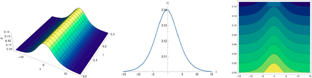
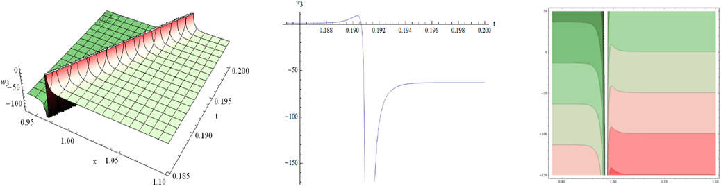
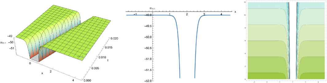
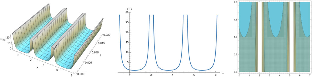
By selecting different parameters, we can get some graphical simulation including the famous bell-shape soliton solutions and blow-up pattern wave solution of system (1) in Figures 1, 2. Some simulation of the above periodic wave solutions are shown in Figures 3, 4.

$c=1,\mu =1,a_0=1,{\gamma }_1=2,{\xi }_0=0,t=0.55.$

$c=1,\mu =1,a_0=2,{\gamma }_1=1,{\xi }_0=100,t=0.42.$

Figure 1

Figure 1. When $\alpha =0.9,\beta =1,k=0.2,b=45,$ $c=45,\mu =40,a_0=0.1,{\gamma }_1=1,{\xi }_0=0,$ t = 0.1, the 3D plot, 2D plot and contour plot of the solitary wave pulse $u_2$.

Figure 2

Figure 2. When $\alpha =0.9,\beta =0.8,k=1,b=c=-2,\mu =1,$ a₀ = b₀ = c₀ = 1, ${\gamma }_1={\gamma }_2=5,{\xi }_0=0,x=1$, the 3D plot, 2D plot and contour plot of the solitary wave pulse $w_3$.

Figure 3

Figure 3. The 3D plot, 2D plot and contour plot of $v_6$ with $\alpha =0.8,\beta =1,k=0.2,b=45,$

Figure 4

Figure 4. The 3D plot, 2D plot and contour plot of $v_7$ with $\alpha =0.9,\beta =1,k=0.4,b=2,$

3.2 Solving Eq. (1) by the $G^{\prime }/\left(bG+G+a\right)$-expansion method

Suppose Equation 5 has solutions of the following form:

$\left\{\begin{array}{l}u=a_0+a_1\left(\frac{G^{\prime }}{b{G}^{\prime }+G+a}\right)+a_2{\left(\frac{G^{\prime }}{b{G}^{\prime }+G+a}\right)}^2=a_0+a_{1}F+a_2{F}^2,\\ v=b_0+b_1\left(\frac{G^{\prime }}{b{G}^{\prime }+G+a}\right)+b_2{\left(\frac{G^{\prime }}{b{G}^{\prime }+G+a}\right)}^2=b_0+b_{1}F+b_2{F}^2,\\ w=c_0+c_1\left(\frac{G^{\prime }}{b{G}^{\prime }+G+a}\right)+c_2{\left(\frac{G^{\prime }}{b{G}^{\prime }+G+a}\right)}^2=c_0+c_{1}F+c_2{F}^2.\end{array}\right.(23)$

Where $a_i,b_i,c_i\left(i=0,1,2\right)$ are constants to be determined.

Substituting Equations 23, 15 into Equation 5, and setting the coefficients $F^i\left(i=0,1,2,3,4,\cdots \right)$ to zero, we could get a set of algebraic equations about $a_i,b_i,c_i,b,\lambda ,\mu ,k,C$. Without losing generality, we let $b=1$:

$\begin{array}{l}{F}^0:-\mathrm{C}\mu a_1+2k^3{\lambda }^2\mu a_1+4k^3{\mu }^2{a}_1-12k^3\lambda {\mu }^2{a}_1+12k^3{\mu }^3{a}_1+6k\mu a_0{a}_1+12k^3\lambda {\mu }^2{a}_2-24k^3{\mu }^3{a}_2-12k\mu b_0{b}_1+6k\mu c_1=0,\\ F:-C\lambda a_1+2k^3{\lambda }^3{a}_1+2C\mu a_1+16k^3\lambda \mu a_1-28k^3{\lambda }^2\mu a_1-32k^3{\mu }^2{a}_1+72k^3\lambda {\mu }^2{a}_1-48k^3{\mu }^3{a}_1+6k\lambda a_0{a}_1-12k\mu a_0{a}_1\\ +6k\mu a_1^2-2C\mu a_2+28k^3{\lambda }^2\mu a_2+32k^3{\mu }^2{a}_2-144k^3\lambda {\mu }^2{a}_2+144k^3{\mu }^3{a}_2+12k\mu a_0{a}_2-12k\lambda b_0{b}_1+24k\mu b_0{b}_1\\ -12k\mu b_1^2-24k\mu b_0{b}_2+6k\lambda c_1-12k\mu c_1+12k\mu c_2=0,\end{array}$

$\begin{array}{l}{F}^2:-C{a}_1+C\lambda a_1+14k^3{\lambda }^2{a}_1-14k^3{\lambda }^3{a}_1-C\mu a_1+16k^3\mu a_1-88k^3\lambda \mu a_1+86k^3{\lambda }^2\mu a_1+88k^3{\mu }^2{a}_1-144k^3\lambda {\mu }^2{a}_1\\ +72k^3{\mu }^3{a}_1+6k{a}_0{a}_1-6k\lambda a_0{a}_1+6k\mu a_0{a}_1+6k\lambda a_1^2-12k\mu a_1^2-2\mathrm{C}\lambda a_2+16k^3{\lambda }^3{a}_2+4C\mu a_2+104k^3\lambda \mu a_2\\ -200k^3{\lambda }^2\mu a_2-208k^3{\mu }^2{a}_2+504k^3\lambda {\mu }^2{a}_2-336k^3{\mu }^3{a}_2+12k\lambda a_0{a}_2-24k\mu a_0{a}_2+18k\mu a_1{a}_2-12k{b}_0{b}_1\\ +12k\lambda b_0{b}_1-12k\mu b_0{b}_1-12k\lambda b_1^2+24k\mu b_1^2-24k\lambda b_0{b}_2+48k\mu b_1{b}_2-36k\mu b_1{b}_2+6k{c}_1-6k\lambda c_1+6k\mu c_1\\ +12k\lambda c_2-24k\mu c_2=0,\\ F^3:24k^3\lambda a_1-48k^3{\lambda }^2{a}_1+24k^3{\lambda }^3{a}_1-48k^3\mu a_1+144k^3\lambda \mu a_1-96k^3{\lambda }^2\mu a_1-96k^3{\mu }^2{a}_1+120k^3\lambda {\mu }^2{a}_1-48k^3{\mu }^3{a}_1\\ +6k{a}_1^2-6k\lambda a_1^2+6k\mu a_1^2-2C{a}_2+2C\lambda a_2+76k^3{\lambda }^2{a}_2-76k^3{\lambda }^3{a}_2-2C\mu a_2+80k^3\mu a_2-464k^3\lambda \mu a_2+460k^3{\lambda }^2\mu a_2\\ +464k^3{\mu }^2{a}_2-768k^3\lambda {\mu }^2{a}_2+384k^3{\mu }^3{a}_2+12k{a}_0{a}_2-12k\lambda a_0{a}_2+12k\mu a_0{a}_2+18k\lambda a_1{a}_2-36k\mu a_1{a}_2+12k\mu a_2^2\\ -12k{b}_1^2+12k\lambda b_1^2-12k\mu b_1^2-24k{b}_0{b}_2+24k\lambda b_0{b}_2-24k\mu b_0{b}_2-36k\lambda b_1{b}_2+72k\mu b_1{b}_2-24k\mu b_2^2+12k{c}_2\\ -12k\lambda c_2+12k\mu c_2=0,\\ F^4:12k^3{a}_1-36k^3\lambda a_1+36k^3{\lambda }^2{a}_1-12k^3{\lambda }^3{a}_1+36k^3\mu a_1-72k^3\lambda \mu a_1+36k^3{\lambda }^2\mu a_1+36k^3{\mu }^2{a}_1-36k^3\lambda {\mu }^2{a}_1\\ +12k^3{\mu }^3{a}_1+108k^3\lambda a_2-216k^3{\lambda }^2{a}_2+108k^3{\lambda }^3{a}_2-216k^3\mu a_2+648k^3\lambda \mu a_2-432k^3{\lambda }^2\mu a_2-432k^3{\mu }^2{a}_2\\ +540k^3\lambda {\mu }^2{a}_2-216k^3{\mu }^3{a}_2+18k{a}_1{a}_2-18k\lambda a_1{a}_2+18k\mu a_1{a}_2+12k\lambda a_2^2-24k\mu a_2^2-36k{b}_1{b}_2+6k\lambda b_1{b}_2\\ -36k\mu b_1{b}_2-24k\lambda b_2^2+48k\mu b_2^2=0,\\ F^5:48k^3{a}_2-144k^3\lambda a_2+144k^3{\lambda }^2{a}_2-48k^3{\lambda }^3{a}_2+144k^3\mu a_2-288k^3\lambda \mu a_2+144k^3{\lambda }^2\mu a_2+144k^3{\mu }^2{a}_2\\ -144k^3\lambda {\mu }^2{a}_2+48k^3{\mu }^3{a}_2+12k{a}_2^2-12k\lambda a_2^2+12k\mu a_2^2-24k{b}_2^2+24k\lambda b_2^2-24k\mu b_2^2=0,\\ F^0:-C\mu b_1-4k^3{\lambda }^2\mu b_1-8k^3{\mu }^2{b}_1+24k^3\lambda {\mu }^2{b}_1-24k^3{\mu }^3{b}_1-6k\mu a_0{b}_1-24k^3\lambda {\mu }^2{b}_2+48k^3{\mu }^3{b}_2=0,\\ F:-C\lambda b_1-4k^3{\lambda }^3{b}_1+2C\mu b_1-32k^3\lambda \mu b_1+56k^3{\lambda }^2\mu b_1+64k^3{\mu }^2{b}_1-144k^3\lambda {\mu }^2{b}_1+96k^3{\mu }^3{b}_1\\ -6k\lambda a_0{b}_1+12k\mu a_0{b}_1-6k\mu a_1{b}_1-2C\mu b_2-56k^3{\lambda }^2\mu b_2-64k^3{\mu }^2{b}_2+288k^3\lambda {\mu }^2{b}_2-288k^3{\mu }^3{b}_2\\ -12k\mu a_0{b}_2=0,\\ F^2:-C{b}_1+C\lambda b_1-28k^3{\lambda }^2{b}_1+28k^3{\lambda }^3{b}_1-C\mu b_1-32k^3\mu b_1+176k^3\lambda \mu b_1-172k^3{\lambda }^2\mu b_1-176k^3{\mu }^2{b}_1\\ +288k^3\lambda {\mu }^2{b}_1-144k^3{\mu }^3{b}_1-6k{a}_0{b}_1+6k\lambda a_0{b}_1-6k\mu a_0{b}_1-6k\lambda a_1{b}_1+12k\mu a_1{b}_1-6k\mu a_2{b}_1\\ -2C\lambda b_2-32k^3{\lambda }^3{b}_2+4C\mu b_2-208k^3\lambda \mu b_2+400k^3{\lambda }^2\mu b_2+416k^3{\mu }^2{b}_2-1008k^3\lambda {\mu }^2{b}_2\\ +672k^3{\mu }^3{b}_2-12k\lambda a_0{b}_2+24k\mu a_0{b}_2-12k\mu a_1{b}_2=0,\\ F^3:-48k^3\lambda b_1+96k^3{\lambda }^2{b}_1-48k^3{\lambda }^3{b}_1+96k^3\mu b_1-288k^3\lambda \mu b_1+192k^3{\lambda }^2\mu b_1+192k^3{\mu }^2{b}_1\\ -240k^3\lambda {\mu }^2{b}_1+96k^3{\mu }^3{b}_1-6k{a}_1{b}_1+6k\lambda a_1{b}_1-6k\mu a_1{b}_1-6k\lambda a_2{b}_1+12k\mu a_2{b}_1-2C{b}_2\\ +2C\lambda b_2-152k^3{\lambda }^2{b}_2+152k^3{\lambda }^3{b}_2-2C\mu b_2-160k^3\mu b_2+928k^3\lambda \mu b_2-920k^3{\lambda }^2\mu b_2\\ -928k^3{\mu }^2{b}_2+1536k^3\lambda {\mu }^2{b}_2-768k^3{\mu }^3{b}_2-12k{a}_0{b}_2+12k\lambda a_0{b}_2-12k\mu a_0{b}_2-12k\lambda a_1{b}_2\\ +24k\mu a_1{b}_2-12k\mu a_2{b}_2=0,\\ F^4:-24k^3{b}_1+72k^3\lambda b_1-72k^3{\lambda }^2{b}_1+24k^3{\lambda }^3{b}_1-72k^3\mu b_1+144k^3\lambda \mu b_1-72k^3{\lambda }^2\mu b_1-72k^3{\mu }^2{b}_1\\ +72k^3\lambda {\mu }^2{b}_1-24k^3{\mu }^3{b}_1-6k{a}_2{b}_1+6k\lambda a_2{b}_1-6k\mu a_2{b}_1-216k^3\lambda b_2+432k^3{\lambda }^2{b}_2\\ -216k^3{\lambda }^3{b}_2+432k^3\mu b_2-1296k^3\lambda \mu b_2+864k^3{\lambda }^2\mu b_2+864k^3{\mu }^2{b}_2-1080k^3\lambda {\mu }^2{b}_2\\ +432k^3{\mu }^3{b}_2-12k{a}_1{b}_2+12k\lambda a_1{b}_2-12k\mu a_1{b}_2-12k\lambda a_2{b}_2+24k\mu a_2{b}_2=0,\\ F^5:-96k^3{b}_2+288k^3\lambda b_2-288k^3{\lambda }^2{b}_2+96k^3{\lambda }^3{b}_2-288k^3\mu b_2+576k^3\lambda \mu b_2-288k^3{\lambda }^2\mu b_2\\ -288k^3{\mu }^2{b}_2+288k^3\lambda {\mu }^2{b}_2-96k^3{\mu }^3{b}_2-12k{a}_2{b}_2+12k\lambda a_2{b}_2-12k\mu a_2{b}_2=0,\\ F^0:-C\mu c_1-4k^3{\lambda }^2\mu c_1-8k^3{\mu }^2{c}_1+24k^3\lambda {\mu }^2{c}_1-24k^3{\mu }^3{c}_1-6k\mu a_0{c}_1-24k^3\lambda {\mu }^2{c}_2+48k^3{\mu }^3{c}_2=0,\\ F:-C\lambda c_1-4k^3{\lambda }^3{c}_1+2C\mu c_1-32k^3\lambda \mu c_1+56k^3{\lambda }^2\mu c_1+64k^3{\mu }^2{c}_1-144k^3\lambda {\mu }^2{c}_1+96k^3{\mu }^3{c}_1\\ -6k\lambda a_0{c}_1+12k\mu a_0{c}_1-6k\mu a_1{c}_1-2C\mu c_2-56k^3{\lambda }^2\mu c_2-64k^3{\mu }^2{c}_2+288k^3\lambda {\mu }^2{c}_2-288k^3{\mu }^3{c}_2\\ -12k\mu a_0{c}_2=0,\\ F^2:-C{c}_1+C\lambda c_1-28k^3{\lambda }^2{c}_1+28k^3{\lambda }^3{c}_1-C\mu c_1-32k^3\mu c_1+176k^3\lambda \mu c_1-172k^3{\lambda }^2\mu c_1-176k^3{\mu }^2{c}_1\\ +288k^3\lambda {\mu }^2{c}_1-144k^3{\mu }^3{c}_1-6k{a}_0{c}_1+6k\lambda a_0{c}_1-6k\mu a_0{c}_1-6k\lambda a_1{c}_1+12k\mu a_1{c}_1-6k\mu a_2{c}_1\\ -2C\lambda c_2-32k^3{\lambda }^3{c}_2+4C\mu c_2-208k^3\lambda \mu c_2+400k^3{\lambda }^2\mu c_2+416k^3{\mu }^2{c}_2-1008k^3\lambda {\mu }^2{c}_2\\ +672k^3{\mu }^3{c}_2-12k\lambda a_0{c}_2+24k\mu a_0{c}_2-12k\mu a_1{c}_2=0,\\ F^3:-48k^3\lambda c_1+96k^3{\lambda }^2{c}_1-48k^3{\lambda }^3{c}_1+96k^3\mu c_1-288k^3\lambda \mu c_1+192k^3{\lambda }^2\mu c_1+192k^3{\mu }^2{c}_1\\ -240k^3\lambda {\mu }^2{c}_1+96k^3{\mu }^3{c}_1-6k{a}_1{c}_1+6k\lambda a_1{c}_1-6k\mu a_1{c}_1-6k\lambda a_2{c}_1+12k\mu a_2{c}_1-2C{c}_2+2C\lambda c_2\\ -152k^3{\lambda }^2{c}_2+152k^3{\lambda }^3{c}_2-2C\mu c_2-160k^3\mu c_2+928k^3\lambda \mu c_2-920k^3{\lambda }^2\mu c_2-928k^3{\mu }^2{c}_2\\ +1536k^3\lambda {\mu }^2{c}_2-768k^3{\mu }^3{c}_2-12k{a}_0{c}_2+12k\lambda a_0{c}_2-12k\mu a_0{c}_2-12k\lambda a_1{c}_2+24k\mu a_1{c}_2\\ -12k\mu a_2{c}_2=0,\end{array}$

$\begin{array}{l}{F}^4:-24k^3{c}_1+72k^3\lambda c_1-72k^3{\lambda }^2{c}_1+24k^3{\lambda }^3{c}_1-72k^3\mu c_1+144k^3\lambda \mu c_1-72k^3{\lambda }^2\mu c_1-72k^3{\mu }^2{c}_1\\ +72k^3\lambda {\mu }^2{c}_1-24k^3{\mu }^3{c}_1-6k{a}_2{c}_1+6k\lambda a_2{c}_1-6k\mu a_2{c}_1-216k^3\lambda c_2+432k^3{\lambda }^2{c}_2-216k^3{\lambda }^3{c}_2\\ +432k^3\mu c_2-1296k^3\lambda \mu c_2+864k^3{\lambda }^2\mu c_2+864k^3{\mu }^2{c}_2-1080k^3\lambda {\mu }^2{c}_2+432k^3{\mu }^3{c}_2-12k{a}_1{c}_2\\ +12k\lambda a_1{c}_2-12k\mu a_1{c}_2-12k\lambda a_2{c}_2+24k\mu a_2{c}_2=0,\\ F^5:-96k^3{c}_2+288k^3\lambda c_2-288k^3{\lambda }^2{c}_2+96k^3{\lambda }^3{c}_2-288k^3\mu c_2+576k^3\lambda \mu c_2-288k^3{\lambda }^2\mu c_2\\ -288k^3{\mu }^2{c}_2+288k^3\lambda {\mu }^2{c}_2-96k^3{\mu }^3{c}_2-12k{a}_2{c}_2+12k\lambda a_2{c}_2-12k\mu a_2{c}_2=0.\end{array}$

After solving the above AEs, we can get the following solutions, where the parameters not specified are arbitrary constants.

$\begin{array}{l}\left(11\right)a_1=0,a_2=-8k^2{\left(-1+\mu \right)}^2,b_1=0,b_2=4k^2{\left(-1+\mu \right)}^2,\lambda =2\mu ,\Delta ={\lambda }^2-4\mu =4\mu \left(\mu -1\right),\\ \hspace{1em}\hspace{1em}\hspace{1em}{c}_1=0,c_2=-8k^2{\left(-1+\mu \right)}^2\left(-2a_0-b_0-8k^2\mu +8k^2{\mu }^2\right),b=1,C=-2\left(3a_{0}k+16k^3\mu -16k^3{\mu }^2\right).\end{array}$

$\begin{array}{l}\left(12\right)b=1,a_1=4k^2\left[{\lambda }^2+2\mu \left(1+\mu \right)-\lambda \left(1+3\mu \right)\right],a_2=-4k^2{\left(1-\lambda +\mu \right)}^2,b_0=0,\\ \hspace{1em}\hspace{1em}\hspace{1em}{b}_1=\pm 2k-{\left(1-\lambda +\mu \right)}^2[2a_0+k^2({\lambda }^2-8\lambda \mu +4\mu \left(1+2\mu \right)]\sqrt{},b_2=0,c_2=0,\\ \hspace{1em}\hspace{1em}\hspace{1em}{c}_1=-4k^2\left[{\lambda }^2+2\mu \left(\mu +1\right)-\lambda \left(1+3\mu \right)\right][2a_0+k^2(\left.{\lambda }^2-8\lambda \mu +4\mu \left(1+2\mu \right)\right],\\ \hspace{1em}\hspace{1em}\hspace{1em}C=-6a_{0}k-4k^3\left({\lambda }^2+2\mu -6\lambda \mu +6{\mu }^2\right).\end{array}$

According to Equations 4, 17, 19, 21, 23, we obtain the following solutions for system (1):

$\left\{\begin{array}{l}{u}_{11}=a_0-8k^2{\left(-1+\mu \right)}^2{F}^2,\\ v_{11}=b_0+4k^2{\left(-1+\mu \right)}^2{F}^2,\\ w_{11}=c_0-8k^2{\left(-1+\mu \right)}^2\left(-2a_0-b_0-8k^2\mu +8k^2{\mu }^2\right)F^2,\\ {\xi }_{11}=\frac{2k\mathrm{\Gamma }\left({\gamma }_2+1\right)}{\beta }{x}^{\beta }-\frac{2\mathrm{\Gamma }\left({\gamma }_1+1\right)}{\alpha }\left(3a_{0}k+16k^3\mu -16k^3{\mu }^2\right)t^{\alpha }+{\xi }_0.\end{array}\right.$

$\left\{\begin{array}{l}{u}_{12}=a_0+4k^2\left[{\lambda }^2+2\mu \left(1+\mu \right)-\lambda \left(1+3\mu \right)\right]F-4k^2{\left(1-\lambda +\mu \right)}^2{F}^2,\\ v_{12}=\pm 2k-{\left(1-\lambda +\mu \right)}^2[2a_0+k^2({\lambda }^2-8\lambda \mu +4\mu \left(1+2\mu \right)]\sqrt{}F,\\ w_{12}=c_0-4k^2\left[{\lambda }^2+2\mu \left(\mu +1\right)-\lambda \left(1+3\mu \right)\right][2a_0+k^2(\left.{\lambda }^2-8\lambda \mu +4\mu \left(1+2\mu \right)\right]F,\\ {\xi }_{12}=\frac{2k\mathrm{\Gamma }\left({\gamma }_2+1\right)}{\beta }{x}^{\beta }-\frac{\mathrm{\Gamma }\left({\gamma }_1+1\right)}{\alpha }\left[6a_{0}k+4k^3\left({\lambda }^2+2\mu -6\lambda \mu +6{\mu }^2\right)\right]t^{\alpha }+{\xi }_0.\end{array}\right.$

We can determine the following solutions.

Case 1: $\Delta >0$, when $\mu <0$ or $\mu >1$.

$\left\{\begin{array}{l}{u}_{11.1}=a_0-8k^2{\left(-1+\mu \right)}^2{\left(1+\frac{2C_1+2C_2{e}^{\sqrt{\Delta }{\xi }_{11.1}}}{C_1\left(-2+\lambda +\sqrt{\Delta }\right)+C_2\left(-2+\lambda -\sqrt{\Delta }\right)e^{\sqrt{\Delta }{\xi }_{11.1}}}\right)}^2,\\ v_{11.1}=b_0+4k^2{\left(-1+\mu \right)}^2{\left(1+\frac{2C_1+2C_2{e}^{\sqrt{\Delta }{\xi }_{11.1}}}{C_1\left(-2+\lambda +\sqrt{\Delta }\right)+C_2\left(-2+\lambda -\sqrt{\Delta }\right)e^{\sqrt{\Delta }{\xi }_{11.1}}}\right)}^2,\\ w_{11.1}=c_0-8k^2{\left(-1+\mu \right)}^2\left(-2a_0-b_0-8k^2\mu +8k^2{\mu }^2\right){\left(1+\frac{2C_1+2C_2{e}^{\sqrt{\Delta }{\xi }_{11.1}}}{C_1\left(-2+\lambda +\sqrt{\Delta }\right)+C_2\left(-2+\lambda -\sqrt{\Delta }\right)e^{\sqrt{\Delta }{\xi }_{11.1}}}\right)}^2,\\ {\xi }_{11.1}=\frac{2k\mathrm{\Gamma }\left({\gamma }_2+1\right)}{\beta }{x}^{\beta }-\frac{2\mathrm{\Gamma }\left({\gamma }_1+1\right)}{\alpha }\left(3a_{0}k+16k^3\mu -16k^3{\mu }^2\right)t^{\alpha }+{\xi }_0.\end{array}\right.$

$\left\{\begin{array}{l}{u}_{12.1}=a_0+4k^2\left[{\lambda }^2+2\mu \left(1+\mu \right)-\lambda \left(1+3\mu \right)\right]\left(1+\frac{2C_1+2C_2{e}^{\sqrt{\Delta }{\xi }_{12.1}}}{C_1\left(-2+\lambda +\sqrt{\Delta }\right)+C_2\left(-2+\lambda -\sqrt{\Delta }\right)e^{\sqrt{\Delta }{\xi }_{12.1}}}\right)\\ -4k^2{\left(1-\lambda +\mu \right)}^2{\left(1+\frac{2C_1+2C_2{e}^{\sqrt{\Delta }{\xi }_{12.1}}}{C_1\left(-2+\lambda +\sqrt{\Delta }\right)+C_2\left(-2+\lambda -\sqrt{\Delta }\right)e^{\sqrt{\Delta }{\xi }_{12.1}}}\right)}^2,\\ v_{12.1}=\pm 2k-{\left(1-\lambda +\mu \right)}^2[2a_0+k^2({\lambda }^2-8\lambda \mu +4\mu \left(1+2\mu \right)]\sqrt{\left(1+\frac{2C_1+2C_2{e}^{\sqrt{\Delta }{\xi }_{12.1}}}{C_1\left(-2+\lambda +\sqrt{\Delta }\right)+C_2\left(-2+\lambda -\sqrt{\Delta }\right)e^{\sqrt{\Delta }{\xi }_{12.1}}}\right)},\\ w_{12.1}=c_0-4k^2\left[{\lambda }^2+2\mu \left(\mu +1\right)-\lambda \left(1+3\mu \right)\right][2a_0+k^2(\left.{\lambda }^2-8\lambda \mu +4\mu \left(1+2\mu \right)\right]\left(1+\frac{2C_1+2C_2{e}^{\sqrt{\Delta }{\xi }_{12.1}}}{C_1\left(-2+\lambda +\sqrt{\Delta }\right)+C_2\left(-2+\lambda -\sqrt{\Delta }\right)e^{\sqrt{\Delta }{\xi }_{12.1}}}\right),\\ {\xi }_{12.1}=\frac{2k\mathrm{\Gamma }\left({\gamma }_2+1\right)}{\beta }{x}^{\beta }-\frac{\mathrm{\Gamma }\left({\gamma }_1+1\right)}{\alpha }\left[6a_{0}k+4k^3\left({\lambda }^2+2\mu -6\lambda \mu +6{\mu }^2\right)\right]t^{\alpha }+{\xi }_0.\end{array}\right.$

Case 2: $\Delta <0$, when $0<\mu <1$.

$\left\{\begin{array}{l}{u}_{11.2}=a_0-8k^2{\left(-1+\mu \right)}^2{\left(\frac{\left(\lambda C_1-\sqrt{-\Delta }{C}_2\right)\cos \left(\frac{\sqrt{-\Delta }}{2}{\xi }_{11.2}\right)+\left(\lambda C_2+\sqrt{-\Delta }{C}_1\right)\sin \left(\frac{\sqrt{-\Delta }}{2}{\xi }_{11.2}\right)}{\left(\left(\lambda -2\right)C_1-\sqrt{-\Delta }{C}_2\right)\cos \left(\frac{\sqrt{-\Delta }}{2}{\xi }_{11.2}\right)+\left(\left(\lambda -2\right)C_2+\sqrt{-\Delta }{C}_1\right)\sin \left(\frac{\sqrt{-\Delta }}{2}{\xi }_{11.2}\right)}\right)}^2,\\ v_{11.2}=b_0+4k^2{\left(-1+\mu \right)}^2{\left(\frac{\left(\lambda C_1-\sqrt{-\Delta }{C}_2\right)\cos \left(\frac{\sqrt{-\Delta }}{2}{\xi }_{11.2}\right)+\left(\lambda C_2+\sqrt{-\Delta }{C}_1\right)\sin \left(\frac{\sqrt{-\Delta }}{2}{\xi }_{11.2}\right)}{\left(\left(\lambda -2\right)C_1-\sqrt{-\Delta }{C}_2\right)\cos \left(\frac{\sqrt{-\Delta }}{2}{\xi }_{11.2}\right)+\left(\left(\lambda -2\right)C_2+\sqrt{-\Delta }{C}_1\right)\sin \left(\frac{\sqrt{-\Delta }}{2}{\xi }_{11.2}\right)}\right)}^2,\\ w_{11.2}=c_0-8k^2{\left(-1+\mu \right)}^2\left(-2a_0-b_0-8k^2\mu +8k^2{\mu }^2\right){\left(\frac{\left(\lambda C_1-\sqrt{-\Delta }{C}_2\right)\cos \left(\frac{\sqrt{-\Delta }}{2}{\xi }_{11.2}\right)+\left(\lambda C_2+\sqrt{-\Delta }{C}_1\right)\sin \left(\frac{\sqrt{-\Delta }}{2}{\xi }_{11.2}\right)}{\left(\left(\lambda -2\right)C_1-\sqrt{-\Delta }{C}_2\right)\cos \left(\frac{\sqrt{-\Delta }}{2}{\xi }_{11.2}\right)+\left(\left(\lambda -2\right)C_2+\sqrt{-\Delta }{C}_1\right)\sin \left(\frac{\sqrt{-\Delta }}{2}{\xi }_{11.2}\right)}\right)}^2,\\ {\xi }_{11.2}=\frac{2k\mathrm{\Gamma }\left({\gamma }_2+1\right)}{\beta }{x}^{\beta }-\frac{2\mathrm{\Gamma }\left({\gamma }_1+1\right)}{\alpha }\left(3a_{0}k+16k^3\mu -16k^3{\mu }^2\right)t^{\alpha }+{\xi }_0.\end{array}\right.$

$\begin{array}{l}\left\{\begin{array}{l}{u}_{12.2}=a_0+4k^2\left[{\lambda }^2+2\mu \left(1+\mu \right)-\lambda \left(1+3\mu \right)\right]F_{12.2}-4k^2{\left(1-\lambda +\mu \right)}^2{F}_{12.2}^2,\\ v_{12.2}=\pm 2k\sqrt{-{\left(1-\lambda +\mu \right)}^2[2a_0+k^2({\lambda }^2-8\lambda \mu +4\mu \left(1+2\mu \right)]}{F}_{12.2},\\ w_{12.2}=c_0-4k^2\left[{\lambda }^2+2\mu \left(\mu +1\right)-\lambda \left(1+3\mu \right)\right]\left[2|a_0|+|k^2\right.(\left.{\lambda }^2-8\lambda \mu +4\mu \left(1+2\mu \right)\right]F_{12.2},\\ {\xi }_{12.2}=\frac{2k\mathrm{\Gamma }\left({\gamma }_2+1\right)}{\beta }{x}^{\beta }-\frac{\mathrm{\Gamma }\left({\gamma }_1+1\right)}{\alpha }\left[6a_{0}k+4k^3\left({\lambda }^2+2\mu -6\lambda \mu +6{\mu }^2\right)\right]t^{\alpha }+{\xi }_0.\end{array}\right.\\ F_{12.2}=\frac{\left(\lambda C_1-\sqrt{-\Delta }{C}_2\right)\cos \left(\frac{\sqrt{-\Delta }}{2}{\xi }_{12.2}\right)+\left(\lambda C_2+\sqrt{-\Delta }{C}_1\right)\sin \left(\frac{\sqrt{-\Delta }}{2}{\xi }_{12.2}\right)}{\left(\left(\lambda -2\right)C_1-\sqrt{-\Delta }{C}_2\right)\cos \left(\frac{\sqrt{-\Delta }}{2}{\xi }_{12.2}\right)+\left(\left(\lambda -2\right)C_2+\sqrt{-\Delta }{C}_1\right)\sin \left(\frac{\sqrt{-\Delta }}{2}{\xi }_{12.2}\right)}.\end{array}$

Case 3: $\Delta =0$, when $\mu =0$.

$\left\{\begin{array}{l}{u}_{11.3}=a_0-8k^2{\left(\frac{2C_2-\lambda C_1-\lambda C_2{\xi }_{11.3}}{2C_2+\left(2-\lambda \right)\left(C_1+C_2\right){\xi }_{11.3}}\right)}^2,\\ v_{11.3}=b_0+4k^2{\left(\frac{2C_2-\lambda C_1-\lambda C_2{\xi }_{11.3}}{2C_2+\left(2-\lambda \right)\left(C_1+C_2\right){\xi }_{11.3}}\right)}^2,\\ w_{11.3}=c_0-8k^2\left(-2a_0-b_0\right){\left(\frac{2C_2-\lambda C_1-\lambda C_2{\xi }_{11.3}}{2C_2+\left(2-\lambda \right)\left(C_1+C_2\right){\xi }_{11.3}}\right)}^2,\\ {\xi }_{11.3}=\frac{2k\mathrm{\Gamma }\left({\gamma }_2+1\right)}{\beta }{x}^{\beta }-\frac{\mathrm{\Gamma }\left({\gamma }_1+1\right)}{\alpha }\left(6a_{0}k\right)t^{\alpha }+{\xi }_0.\end{array}\right.$

$\left\{\begin{array}{l}{u}_{12.3}=a_0+4k^2\left({\lambda }^2-\lambda \right)\frac{2C_2-\lambda C_1-\lambda C_2{\xi }_{12.3}}{2C_2+\left(2-\lambda \right)\left(C_1+C_2\right){\xi }_{12.3}}-4k^2{\left(1-\lambda \right)}^2{\left(\frac{2C_2-\lambda C_1-\lambda C_2{\xi }_{12.3}}{2C_2+\left(2-\lambda \right)\left(C_1+C_2\right){\xi }_{12.3}}\right)}^2,\\ v_{12.3}=\pm 2k\sqrt{-{\left(1-\lambda \right)}^2\left(2a_0+k^2{\lambda }^2\right)}\frac{2C_2-\lambda C_1-\lambda C_2{\xi }_{12.3}}{2C_2+\left(2-\lambda \right)\left(C_1+C_2\right){\xi }_{12.3}},\\ w_{12.3}=c_0-4k^2\left({\lambda }^2-\lambda \right)\left(2a_0+k^2{\lambda }^2\right)\frac{2C_2-\lambda C_1-\lambda C_2\xi }{2C_2+\left(2-\lambda \right)\left(C_1+C_2\right){\xi }_{12.3}},\\ {\xi }_{12.3}=\frac{2k\mathrm{\Gamma }\left({\gamma }_2+1\right)}{\beta }{x}^{\beta }-\frac{\mathrm{\Gamma }\left({\gamma }_1+1\right)}{\alpha }\left(6a_{0}k+4k^3{\lambda }^2\right)t^{\alpha }+{\xi }_0.\end{array}\right.$

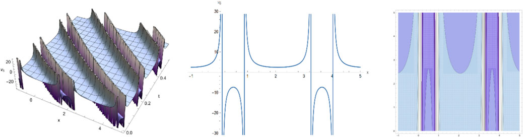
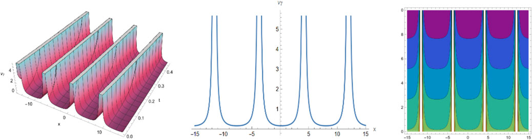
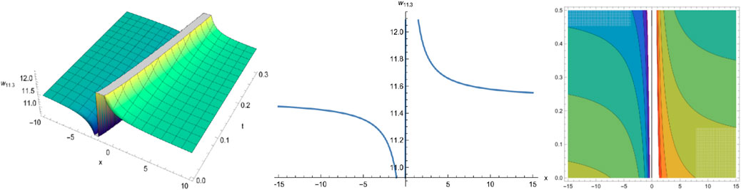
Selecting different parameters, we can get some graphical simulation of above solutions $\alpha =1,\beta =1$ (Figures 5, 6) and $\alpha =0.8,\beta =1$ (Figure 7) as follows:

${\gamma }_1=0,{\xi }_0=0,t=0.02,C_1=1,C_2=2.$

${\gamma }_1=0,{\xi }_0=0,t=0.02,C_1=1,C_2=2.$

${\gamma }_1=1,{\xi }_0=10,t=0.12,C_1=3,C_2=0.3.$

Figure 5

Figure 5. The 3D plot, 2D plot and contour plot of $u_{11.1}$ with $\mu =3,\lambda =6,k=1,b_0=1,c_0=1,a_0=1,$

Figure 6

Figure 6. The 3D plot, 2D plot and contour plot of $v_{11.2}$ with $\mu =\frac{1}{2},\lambda =1,k=1,b_0=1,c_0=1,a_0=1,$

Figure 7

Figure 7. The 3D plot, 2D plot and contour plot of $w_{11.3}$ with $\mu =0,\lambda =1.5,k=3,b_0=1,c_0=10,a_0=3,$

Remark 5. All of the above results have been checked by computer programs, and they are founded for the first time to our knowledge.

3.3 Results and discussion

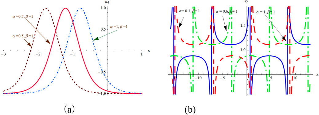
We have obtained many types of new analytical solutions of the system (1) by two efficient methods, which include the famous bell-shaped solitary wave $u_2$, this smooth solution reveals a balance of nonlinear effects and dispersion effects, the blow-up wave $w_3$ which is distorted between the interval (0.190, 0.192) etc. There are also many forms of periodic waves, and these periodic wave solutions embody different properties. For example, the waveform of $v_6$ alternates up and down in both directions, periodicity of $v_7$ and $v_{11.2}$ are only reflected in one direction. If we choose different parameters and orders, we could find that the waveform of system (1) will evolve with time $t$. The Figures (a) and (b) in Figure 8 show the evolutionary process of $u_4,v_6$ with time fractional order with parameters $a_0=b_0=c_0=1,b=1,c=1,\mu =1,k=-1,t=1,{\gamma }_1={\gamma }_2=2,\beta =1$ and $a_0=b_0=c_0=1,$ $b=45,c=1,\mu =1,k=0.2,t=0.55,{\gamma }_1=2,$ ${\gamma }_2=0,\beta =1$ respectively. Numerical simulations show that the waveform shifts to the right as the time order increases, and these properties may be of great significance for revealing the internal structure of system (1). However, In MEMS, the understanding of nonlinear wave phenomena and the availability of exact solutions can contribute to the design and optimization of various components. For example, in MEMS sensors, these solutions can help analyze the response to external stimuli and improve the sensitivity and accuracy.

Figure 8

Figure 8. Fractional evolution of u₄ in (A) and v₆ in (B) over time under different parameters.

4 Conclusion

In conclusion, by utilizing the modified $\left(G^{\prime }/G,1/G\right)$-expansion method, the $G^{\prime }/\left(b{G}^{\prime }+G+a\right)$-expansion method and the travelling wave transform under the definition of M fractional derivative, twelve new types of exact solutions of the generalized time-space fractional coupled Hirota-Satsuma KdV system are obtained successfully. These solutions include complex solitary wave solutions, trigonometric periodic wave solutions, and rational function solutions. These solutions can be transformed into integer order cases under special parameter selection, and they have important theoretical guiding value for profoundly revealing the interaction between two nonlinear long waves with different dispersion effects. The waveforms of partial solutions and their characteristic images of time evolution are obtained by numerical simulation. It is proved by practice that these two methods can be applied to many other nonlinear equations including the MEMS. Additionally, in integrated MEMS systems, the knowledge of these solutions can enhance the functionality and reliability. However, the proposed definition of M-fractional derivatives still has some limitations, and it is difficult to characterize the necessary connection between two real number or complex number order derivatives. On the other hand, the unified definition of fractional derivatives definition needs to be further explored and developed for us in the future. Once our definition has been substantially refined, then we work on perturbation theory, dynamical system theory, soliton theory, etc., will be better developed [63–65]. How to extend this method to discretely-coupled nonlinear systems with arbitrary subhigher dimensions is still worth further study. This will open up new avenues for exploring more complex nonlinear phenomena and expanding the application scope of these methods in the field of nano/micro devices and systems.

Data availability statement

The original contributions presented in the study are included in the article/supplementary material, further inquiries can be directed to the corresponding author.

Author contributions

YC: Funding acquisition, Investigation, Supervision, Writing–original draft, Formal Analysis. SH: Methodology, Resources, Writing–review and editing, Conceptualization, Project administration. SY: Conceptualization, Data curation, Writing–original draft, Formal Analysis, Visualization. XC: Formal Analysis, Investigation, Methodology, Resources, Writing–review and editing. JY: Conceptualization, Project administration, Visualization, Writing–original draft.

Funding

The author(s) declare that financial support was received for the research, authorship, and/or publication of this article. This work is partially supported by the practical innovation training program projects for the university students of Jiangsu Province (Grant No. 202410299873X).

Conflict of interest

The authors declare that the research was conducted in the absence of any commercial or financial relationships that could be construed as a potential conflict of interest.

Generative AI statement

The author(s) declare that no Generative AI was used in the creation of this manuscript.

Publisher’s note

All claims expressed in this article are solely those of the authors and do not necessarily represent those of their affiliated organizations, or those of the publisher, the editors and the reviewers. Any product that may be evaluated in this article, or claim that may be made by its manufacturer, is not guaranteed or endorsed by the publisher.

References

1. Haq A. Partial-approximate controllability of semi-linear systems involving two Riemann-Liouville fractional derivatives. Chaos, Solitons and Fractals (2022) 157:111923. doi:10.1016/j.chaos.2022.111923

CrossRef Full Text | Google Scholar

2. Caputo M. Linear models of dissipation whose Q is almost frequency independent-II. Geophys J Int (1967) 13:529–39. doi:10.1111/j.1365-246x.1967.tb02303.x

CrossRef Full Text | Google Scholar

3. Guner O, Atik H, Kayyrzhanovich AA. New exact solution for space-time fractional differential equations via G'/G-expansion method. Optik (2017) 130:696–701. doi:10.1016/j.ijleo.2016.10.116

CrossRef Full Text | Google Scholar

4. Atangana A, Baleanu D, Alsaedi A. Analysis of time-fractional Hunter-Saxton equation: a model of neumatic liquid crystal. Open Phys (2016) 14:145–9. doi:10.1515/phys-2016-0010

CrossRef Full Text | Google Scholar

5. Atangana A, Koca I. Chaos in a simple nonlinear system with Atangana-Baleanu derivatives with fractional order. Chaos, Solitons and Fractals (2016) 89:447–54. doi:10.1016/j.chaos.2016.02.012

CrossRef Full Text | Google Scholar

6. Khalil R, Al Horani M, Yousef A, Sababheh M. A new definition of fractional derivative. J Comput Appl Mathematics (2014) 264:65–70. doi:10.1016/j.cam.2014.01.002

CrossRef Full Text | Google Scholar

7. Shady MA, Kaabar MKA. A novel computational tool for the fractional-order special functions arising from modeling scientific phenomena via Abu-Shady-Kaabar fractional derivative. Comput Math Methods Med (2022) 2022:2138775. doi:10.1155/2022/2138775

PubMed Abstract | CrossRef Full Text | Google Scholar

8. He JH. Fractal calculus and its geometrical explanation. Results Phys (2018) 10:272–6. doi:10.1016/j.rinp.2018.06.011

CrossRef Full Text | Google Scholar

9. He JH. A tutorial review on fractal spacetime and fractional calculus. Int J Theor Phys (2014) 53:3698–718. doi:10.1007/s10773-014-2123-8

CrossRef Full Text | Google Scholar

10. Nadeem M, Ahmad J, Nusrat F, Iambor LF. Fuzzy solutions of some variants of the fractional order Korteweg-de-Vries equations via an analytical method. Alexandria Eng J (2023) 80:8–21. doi:10.1016/j.aej.2023.08.012

CrossRef Full Text | Google Scholar

11. Tajadodi H. A Numerical approach of fractional advection-diffusion equation with Atangana Baleanu derivative. Chaos, Solitons and Fractals (2020) 130:109527. doi:10.1016/j.chaos.2019.109527

CrossRef Full Text | Google Scholar

12. Yusuf A, Inc M, Aliyu AI, Baleanu D. Optical solitons possessing beta derivative of the Chen-Lee-Liu equation in optical fibers. Front Phys (2019) 7:00034. doi:10.3389/fphy.2019.00034

CrossRef Full Text | Google Scholar

13. Khater MMA, Ghanbari B, Nisar KS, Kumar D. Novel exact solutions of the fractional Bogoyavlensky -Konopelchenko equation involving the Atangana-Baleanu-Riemann derivative. Alexandria Eng J (2020) 59:2957–67. doi:10.1016/j.aej.2020.03.032

CrossRef Full Text | Google Scholar

14. Madiha S, Muhammad A, Farah AA, Majeed A, Abdeljawad T, Alqudah MA. Numerical solutions of time fractional Burgers equation involving Atangana-Baleanu derivative via cubic B-spline functions. Results Phys (2022) 34:105244. doi:10.1016/j.rinp.2022.105244

CrossRef Full Text | Google Scholar

15. Nadeem M, Alsayaad Y. A new study for the investigation of nonlinear fractional drinfeld–sokolov–wilson equation. Math Probl Eng (2023) 2023(1):9274115. doi:10.1155/2023/9274115

CrossRef Full Text | Google Scholar

16. Hu XB, Wang DL, Tam HW. Lax pairs and Bäcklund transformations for a coupled Ramani equation and its related system. Appl Mathematics Lett (2000) 13:45–8. doi:10.1016/s0893-9659(00)00052-5

CrossRef Full Text | Google Scholar

17. Liu CP. A Modified homogeneous balance method and its applications. Commun Theor Phys (2011) 56(08):223–7. doi:10.1088/0253-6102/56/2/05

CrossRef Full Text | Google Scholar

18. Huang Q, Wang LZ, Zuo SL. Consistent riccati expansion method and its applications to nonlinear fractional partial differential equations. Commun Theor Phys (2016) 65(02):177–84. doi:10.1088/0253-6102/65/2/177

CrossRef Full Text | Google Scholar

19. Ebaid A, Aly EH. Exact solutions for the transformed reduced Ostrovsky equation via the -expansion method in terms of Weierstrass-elliptic and Jacobian-elliptic functions. Wave Motion (2012) 49:296–308. doi:10.1016/j.wavemoti.2011.11.003

CrossRef Full Text | Google Scholar

20. Hong BJ. New Jacobi elliptic functions solutions for the variable-coefficient mKdV equation. Appl Math Comput (2009) 215(8):2908–13. doi:10.1016/j.amc.2009.09.035

CrossRef Full Text | Google Scholar

21. Mohanty SK, Kravchenko OV, Dev AN. Exact traveling wave solutions of the Schamel Burgers equation by using generalized-improved and generalized (G'/G)-expansion methods. Results Phys (2022) 33:105124. doi:10.1016/j.rinp.2021.105124

CrossRef Full Text | Google Scholar

22. Matveev VA, Salle MA. Darboux transformations and solitons. Berlin, Heidelberg: Springer Verlag (1991).

Google Scholar

23. Nass AM. Lie symmetry analysis and exact solutions of fractional ordinary differential equations with neutral delay. Appl Mathematics Comput (2019) 347:370–80. doi:10.1016/j.amc.2018.11.002

CrossRef Full Text | Google Scholar

24. Rach R. On the Adomian(decomposition) method and comparisions with Picard’s method. J Math Anal Appl (1987) 128:480–3. doi:10.1112/S1461157017000018

CrossRef Full Text | Google Scholar

25. He JH. Homotopy perturbation technique. Comput Methods Appl Mech Eng (1999) 178:257–62. doi:10.1016/s0045-7825(99)00018-3

CrossRef Full Text | Google Scholar

26. Ramos JI. On the variational iteration method and other iterative techniques for nonlinear differential equations. Appl Mathematics Comput (2008) 199:39–69. doi:10.1016/j.amc.2007.09.024

CrossRef Full Text | Google Scholar

27. He CH, Liu HW, Liu C. A fractal-based approach to the mechanical properties of recycled aggregate concretes. Facta Universitatis, Ser Mech Eng (2024) 22(2):329–42. doi:10.22190/fume240605035h

CrossRef Full Text | Google Scholar

28. He CH, Liu C. Fractal dimensions of a porous concrete and its effect on the concrete’s strength. Facta Universitatis Ser Mech Eng (2023) 21(1):137–50. doi:10.22190/fume221215005h

CrossRef Full Text | Google Scholar

29. Yang XJ. New general fractional-order rheological models with kernels of Mittag-Leffler functions. Rom Rep Phys (2017) 69(4):118.

Google Scholar

30. Meng G, Zhang WM, Huang H, Li HG, Chen D. Micro-rotor dynamics for micro-electro-mechanical systems (MEMS). Chaos, Solitons and Fractals (2009) 40(2):538–62. doi:10.1016/j.chaos.2007.08.003

CrossRef Full Text | Google Scholar

31. Jindal SK, Varma MA, Thukral D. Comprehensive assessment of MEMS double touch mode capacitive pressure sensor on utilization of SiC film as primary sensing element: mathematical modelling and numerical simulation. Microelectronics J (2018) 73:30–6. doi:10.1016/j.mejo.2018.01.002

CrossRef Full Text | Google Scholar

32. Aghababa MP. Chaos in a fractional-order micro-electro-mechanical resonator and its suppression. Chin Phys B (2012) 21(10):100505. doi:10.1088/1674-1056/21/10/100505

CrossRef Full Text | Google Scholar

33. Yaghoubi Z, Adeli M. Adaptive observer-based control for fractional-order chaotic MEMS system. IET Control Theor Appl (2023) 17(11):1586–98. doi:10.1049/cth2.12495

CrossRef Full Text | Google Scholar

34. He JH. Periodic solution of a micro-electromechanical system. Facta Universititatis. Ser Mech Eng (2024) 22(2):187–98. doi:10.22190/fume240603034h

CrossRef Full Text | Google Scholar

35. Sousa JVDC, de Oliveira EC. A new truncated M-fractional derivative type unifying some fractional derivative types with classical properties. Int J Anal Appl (2018) 16(Number 1):83–96. doi:10.48550/arXiv.1704.08187

CrossRef Full Text | Google Scholar

36. Hong BJ, Wang JH. Exact solutions for the generalized Atangana-Baleanu-Riemann fractional (3 + 1)-dimensional Kadomtsev-Petviashvili equation. Symmetry (2023) 15(3):3–15. doi:10.3390/sym15010003

CrossRef Full Text | Google Scholar

38. Hong BJ. Abundant explicit solutions for the M-fractionalgeneralized coupled nonlinear Schrödinger KdV equations. J Low Frequency Noise,Vibration Active Control (2023) 42(3):1222–41. doi:10.1177/14613484221148411

CrossRef Full Text | Google Scholar

39. Hong BJ, Zhou JX, Zhu XC, Wang YT. Some Novel Optical Solutions for the Generalized M-Fractional Coupled NLS System. J Funct Spaces (2023) 2023:8283092. doi:10.1155/2023/8283092

CrossRef Full Text | Google Scholar

40. Hong BJ. Assorted exact explicit solutions for the generalized Atangana’s fractional BBM–Burgers equation with the dissipative term. Front Phys (2022) 10:1071200. doi:10.3389/fphy.2022.1071200

CrossRef Full Text | Google Scholar

41. Wang ML, Zhou YB, Li ZB. Application of a homogeneous balance method to exact solutions of nonlinear equations in mathematical physics. Phys Lett A (1996) 16(2):67–75. doi:10.1016/0375-9601(96)00283-6

CrossRef Full Text | Google Scholar

42. Salahshour S, Ahmadian A, Abbasbandy S, Baleanu D. M-fractional derivative under interval uncertainty: theory, properties and applications. Chaos, Solitons and Fractals (2018) 117:84–93. doi:10.1016/j.chaos.2018.10.002

CrossRef Full Text | Google Scholar

43. Yao SW, Manzoor R, Zafar A, Inc M, Abbagari S, Houwe A. Exact soliton solutions to the Cahn-Allen equation and Predator-Prey model with truncated M-fractional derivative. Results Phys (2022) 37:105455. doi:10.1016/j.rinp.2022.105455

CrossRef Full Text | Google Scholar

44. Abazari R, Abazari M. Numerical simulation of generalized Hirota-Satsuma coupled KdV equation by RDTM and comparison with DTM. Commun Nonlinear Sci Numer Simulation (2012) 17:619–29. doi:10.1016/j.cnsns.2011.05.022

CrossRef Full Text | Google Scholar

45. Hirota R, Satsuma J. Soliton solutions of a coupled Korteweg-de Vries equation. Phys Lett A (1981) 85:407–8. doi:10.1016/0375-9601(81)90423-0

CrossRef Full Text | Google Scholar

46. Wu YT, Geng XG, Hu XB, Zhu SM. A generalized HirotaSatsuma coupled Korteweg-de Vries equation and miura transformations. Phys Lett A (1999) 255:259–64. doi:10.1016/s0375-9601(99)00163-2

CrossRef Full Text | Google Scholar

47. Fan EG, Hon BYC. Double periodic solutions with Jacobi elliptic functions for two generalized HirotaCSatsuma coupled KdV systems. Phys Lett A (2002) 292:335–7. doi:10.1016/S0375-9601(01)00815-5

CrossRef Full Text | Google Scholar

48. Lu DC, Hong BJ, Tian LX. New explicit exact solutions for the generalized coupled Hirota-Satsuma KdV system. Comput Mathematics Appl (2007) 53(8):1181–90. doi:10.1016/j.camwa.2006.08.047

CrossRef Full Text | Google Scholar

49. Hong BJ. New exact Jacobi elliptic functions solutions for the generalized coupled Hirota-Satsuma KdV system. Appl Mathematics Comput (2010) 217:472–9. doi:10.1016/j.amc.2010.05.079

CrossRef Full Text | Google Scholar

50. Hu HC, Liu QP. New Darboux transformation for HirotaCSatsuma coupled KdV system. Chaos Solitions and Fractals (2003) 17:921–8. doi:10.1016/S0960-0779(02)00309-0

CrossRef Full Text | Google Scholar

51. Wu LP, Chen SF, Pang CP. Bifurcations of traveling wave solutions for the generalized coupled Hirota-Satsuma KdV system. Nonlinear Anal (2008) 68:3860–9. doi:10.1016/j.na.2007.04.025

CrossRef Full Text | Google Scholar

52. Kurt A, Rezazadeh H, Senol M, Neirameh A, Tasbozan O, Eslami M, et al. Two effective approaches for solving fractional generalized Hirota-Satsuma coupled KdV system arising in interaction of long waves. J Ocean Eng Sci (2019) 4:24–32. doi:10.1016/j.joes.2018.12.004

CrossRef Full Text | Google Scholar

53. Rezazadeh H, Seadawy AR, Eslami M, Mirzazadeh M. Generalized solitary wave solutions to the time fractional generalized Hirota-Satsuma coupled KdV via new definition for wave transformation. J Ocean Eng Sci (2019) 4:77–84. doi:10.1016/j.joes.2019.01.002

CrossRef Full Text | Google Scholar

54. Yan ZY. The extended Jacobian elliptic function expansion method and its application in the generalized Hirota-Satsuma coupled KdV system. Chaos Solitions and Fractals (2003) 15:575–83. doi:10.1016/s0960-0779(02)00145-5

CrossRef Full Text | Google Scholar

55. Zayed EME, Zedan HA, Gepreel KA. On the solitary wave solutions for nonlinear Hirota-Satsuma coupled KdV of equations. Chaos Solitions and Fractals (2004) 22:285–303. doi:10.1016/j.chaos.2003.12.045

CrossRef Full Text | Google Scholar

56. Dogan K. Solitary wave solutions for a generalized Hirota-Satsuma coupled KdV equation. Appl Mathematics Comput (2004) 147:69–78. doi:10.1016/s0096-3003(02)00651-3

CrossRef Full Text | Google Scholar

57. Chen Y, Yan ZY, Li B, Zhang HQ. New explicit solitary wave solutions and periodic wave solutions for the generalized coupled Hirota-Satsuma KdV system. Commun Theor Phys (2002) 38:261–6. doi:10.1088/0253-6102/38/3/261

CrossRef Full Text | Google Scholar

58. Feng Y, Zhang HQ. A new auxiliary function method for solving the generalized coupled Hirota-Satsuma KdV system. Appl Mathematics Comput (2008) 200:283–8. doi:10.1016/j.amc.2007.11.007

CrossRef Full Text | Google Scholar

59. Zuo JM, Zhang YM. Application of the G'/G-expansion method to solve coupled MKdV equations and coupled Hirota-Satsuma coupled KdV equations. Appl Mathematics Comput (2011) 217:5936–41. doi:10.1016/j.amc.2010.12.104

CrossRef Full Text | Google Scholar

60. Guo SM, Zhou YB. The extended G'/G-expansion method and its applications to the Whitham Broer-Kaup-Like equations and coupled Hirota-Satsuma KdV equations. Appl Mathematics Comput (2010) 215:3214–21. doi:10.1016/j.amc.2009.10.008

CrossRef Full Text | Google Scholar

61. Mirhosseini-Alizamini SM, Ullah N, Sabi J, Rezazadeh H, Inc M. New exact solutions for nonlinear Atangana conformable Boussinesq-like equations by new Kudryashov method. Int J Mod Phys B (2021) 35(12):2150163. doi:10.1142/s0217979221501630

CrossRef Full Text | Google Scholar

62. Hosseini K, Bekir A, Ansari R. New exact solutions of the conformable time-fractional Cahn- Allen and Cahn-Hilliard equations using the modified Kudryashov method. Optik (2017) 132:203–9. doi:10.1016/j.ijleo.2016.12.032

CrossRef Full Text | Google Scholar

63. Nadeem M, Li Z. Yang transform for the homotopy perturbation method: promise for fractal-fractional models. Fractals (2023) 31(07):2350068. doi:10.1142/s0218348x23500688

CrossRef Full Text | Google Scholar

64. Nadeem M, Ain QT, Alsayaad Y. Approximate solutions of multidimensional wave problems using an effective approach. J Funct Spaces (2023) 2023(1):5484241–9. doi:10.1155/2023/5484241

CrossRef Full Text | Google Scholar

65. Rafikov M, Balthazar JM. Optimal pest control problem in population dynamics. Comput Appl Mathematics (2005) 24(1):65–81. doi:10.1590/s1807-03022005000100004

CrossRef Full Text | Google Scholar