Double array system identification research based on LSTM neural network

The earthquake simulation shaking table array is an important experimental equipment with a wide range of applications in the field of earthquake engineering. To efficiently address the complex nonlinear problems associated with earthquake simulation shaking array systems, this paper proposes the identification of the earthquake simulation shaking array system using the Long Short-Term Memory (LSTM) algorithm. A dual array system model with flexible specimen connections is established, and this system is identified using the LSTM neural network. The LSTM neural network was validated for identifying the dual array closed-loop system of the earthquake simulation shaking table by using three natural waves and one artificial wave. The results demonstrated that the similarity between the predicted output and the theoretical output of the network identified by LSTM exceeded 0.999. This indicates that the algorithm can accurately reproduce the characteristics of the shaking table itself and shows good performance in time series prediction and data mining. References for earthquake simulation shaking array system experiments are provided.

1 Introduction

The earthquake simulation shaking table is a key laboratory tool for studying and evaluating the seismic resistance of structures. It generates horizontal, vertical, and multidimensional accelerations through a driven platform, simulating the impact of seismic waves on buildings and other structures [1]. The earthquake simulation shaking table array comprises multiple independent earthquake simulation shaking tables that work together to simulate more realistic and complex ground motions. Each table can also be controlled independently to achieve more accurate earthquake wave simulations [2]. Due to factors such as high investment, expensive maintenance and experimental costs, and long construction periods, it is clearly unreasonable to infinitely increase the size and scale of shaking table. Additionally, due to similarity ratios, simply enlarging the shaking table cannot fully meet the requirements. For large-span structures such as bridges, pipelines, aqueducts, and transmission lines, combining multiple small shaking table arrays can be used for testing. The construction and research of shaking table array systems are becoming a trend in both domestic and international research. Gao Chunhua [3] conducted a survey and comparative analysis of various algorithms for domestic shaking tables, summarized the construction forms and loading methods of shaking table substructure tests, as well as the construction and control technical difficulties of shaking table array systems. Ji Jinbao [4, 5] et al. summarized and introduced the functions and characteristics of the shaking table array control system using the nine sub array of Beijing University of Technology as an example, and conducted large-span spatial structure model tests using the equipment. They pointed out the issues and areas that need improvement in using the shaking table array system and explored the relevant research and development of control technology for multi-shaking table array systems. Tao Dehuai [6] conducted a dynamic analysis of the foundation of a dual-array earthquake simulation shaking table and found that the impact of shaking on the foundation remained essentially unchanged under different load conditions. Guan Guangfeng [7] et al. conducted a detailed analysis of different control strategies for a dual array shaking table system and verified the effectiveness of the array system controller through experiments.

The nonlinear influence of shaking table system has always existed in earthquake simulation shaking table test, and has seriously affected its reproduction accuracy and waveform reproduction ability [8, 9]. For more complex shaking table array systems, due to the simultaneous operation of a large number of actuators, the existing control methods cannot meet the requirements for system stability and synchronization [10]. This means that more advanced intelligent control algorithms are needed. As a type of intelligent algorithm, neural network algorithms have good adaptive and generalization abilities, can model and handle nonlinear problems [11–13], and perform well in the control of seismic simulation shaking tables. Gao Chunhua [14, 15] et al. carried out parameter optimization and parameter identification for seismic simulation shaker by intelligent control algorithm, and simulation results showed that the intelligent control algorithm could optimize control parameters, identify multiple parameters, and improve the control effect of the shaker. Yu Shipin [16] et al. used a BP neural network to optimize the control instructions so that the control peak and valley values reached the expected values. Byung Kwan Oh [17] et al. proposed a new model for earthquake response prediction of buildings based on the correlation between ground motion and structure using neural networks. They verified the effectiveness of the proposed neural network model by studying its response prediction performance. A. Zeroual [18] et al. proposed an artificial neural network model, applied it to the prediction of the safety factor for a new earth dam dataset, and compared the predicted results with the stability calculation results of different limit equilibrium slopes. The comparison proved that the prediction ability of the artificial neural network model for the safety factor is satisfactory. Long Short-Term Memory network (LSTM) is a special type of recurrent neural network (RNN) that efficiently processes and predicts sequence data by introducing gating mechanisms. LSTM is designed to solve the problem of gradient vanishing or gradient explosion encountered by traditional RNNs when processing long sequences of data [19]. LSTM can learn long-term dependencies, which is difficult for traditional RNNs to achieve. It is easy to integrate into network structures and is suitable for various time series prediction tasks. Compared with other methods for solving long series problems (such as bidirectional RNNs), LSTM requires fewer parameters. Zhang Wenpeng [20] et al. proposed a three-parameter control parameter tuning algorithm for shakers based on LSTM and adopted the gradient descent method for offline tuning of control parameters. This was combined with the original parameters of the control system for real machine verification. The results showed that the proposed tuning method can achieve better results than manual tuning, and the tuning process is completed offline by the system model without real machine operation, offering advantages of high efficiency and good effect. Ruiyang Zhang [21] et al. proposed two long short-term memory (LSTM) network schemes aimed at data-driven structural seismic response modeling. The verification results show that the proposed LSTM network is a promising, reliable, and computationally efficient method for nonlinear structural response prediction. It has great potential in the reliability assessment of seismic vulnerability analysis of buildings.

System identification is the process of analyzing the input and output data of a system to obtain the mathematical model or dynamic characteristics of the system. This process includes determining the transfer function, state-space model, or other mathematical descriptions of the system. Effective system identification is the key to realize high performance control of shaking table [22, 23]. Zhan Pengyun [24] et al. used the least squares method to identify the model parameters of the shaking table model for seismic simulation. The research shows that the identified model can well reproduce the characteristics of the shaking table system itself, and the least squares identification method can be used to identify the hydraulic and control systems of the shaking table for seismic simulation. Ji Jinbao [25] et al. trained and tested a constructed LSTM network model based on the shaking table system model. The test results show that the LSTM network can reproduce the characteristics of a single-axis open-loop system and can be used as the control object for system simulation and algorithm testing. Febina Christudas [26] et al. utilized input-output data of long short-term memory recurrent neural networks (LSTM-RNN) to model real-time CTS. Compared with empirical models, the LSTM-RNN model achieved better modeling results. Wei Guo [27] et al. developed a physics-guided long short-term memory (PhyLSTM) network for system identification of shaking tables. After detailed hyperparameter testing, the performance of the PhyLSTM model significantly outperformed that of traditional transfer function models.

Based on the above analysis, this paper designs a system identification scheme for a dual-array seismic simulation shaking table based on LSTM neural networks. The LSTM is used to identify the multi-parameter control closed-loop system of the dual array. By comparing the predicted results after neural network training with theoretical results, the feasibility and high research value of this identification scheme are verified.

2 Shaking table two-array system modeling

2.1 Two array system with flexible connection of specimens

For the two-array system, the forces acting on the shaking table platform include not only the actuator forces and the interaction forces between the specimen and the platform but also the additional forces generated due to the asynchronous movement of the two sub-shaking tables. Taking the dual-array system with a flexible connection of the specimen as an example, Figure 1 shows a schematic diagram of the mechanical model of the dual-array system with the specimen.

Figure 1

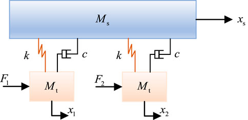
Figure 1. The mechanical model of two-array flexible connection of specimens.

The mass of the specimen in the system is $M_s$, the mass of the shaking table is $M_t$, $k$ is the stiffness coefficient of the connection of the two sub-tables, $c$ is the damping coefficient; The outputs of the two shaker exciter are $F_1$ and $F_2$ respectively, and the displacements of the two tables are $x_1$ and $x_2$ respectively. Assuming the displacement of the specimen is $x_s$, the force balance Equation 1 of the two-array system can be obtained:

$\left\{\begin{array}{l}{M}_{\mathrm{s}}{s}^2{x}_{\mathrm{s}}+\left(cs+k\right)\left(x_{\mathrm{s}}-x_1\right)+\left(cs+k\right)\left(x_{\mathrm{s}}-x_2\right)=0\\ M_{\mathrm{t}}{s}^2{x}_1+\left(cs+k\right)\left(x_1-x_{\mathrm{s}}\right)=F_1\\ M_{\mathrm{t}}{s}^2{x}_2+\left(cs+k\right)\left(x_2-x_{\mathrm{s}}\right)=F_2\end{array}\right.(1)$

The acceleration response of the two sub-stations can be obtained as follows:

$\left\{\begin{array}{l}{s}^2{x}_1=\frac{F_1+\frac{{\left(cs+k\right)}^2}{M_{\mathrm{s}}{s}^2+2cs+2k}{x}_2}{M_{\mathrm{t}}+\frac{cs+k}{s^2}-\frac{{\left(cs+k\right)}^2}{\left(M_{\mathrm{s}}{s}^2+2cs+2k\right)s^2}}\\ s^2{x}_2=\frac{F_2+\frac{{\left(cs+k\right)}^2}{M_{\mathrm{s}}{s}^2+2cs+2k}{x}_1}{M_{\mathrm{t}}+\frac{cs+k}{s^2}-\frac{{\left(cs+k\right)}^2}{\left(M_{\mathrm{s}}{s}^2+2cs+2k\right)s^2}}\end{array}\right.(2)$

There is a coupling between the two expressions in Equation 2, in other words, the displacement $x_1$ of shaker 1 depends not only on the parameters of the shaker itself, but also on the displacement $x_2$ of shaker 2. Next, because the output of the exciter meets Equation 3:

$\left\{\begin{array}{l}{A}_{\mathrm{p}}{p}_{\mathrm{L}1}=F_1\\ A_{\mathrm{p}}{p}_{\mathrm{L}2}=F_2\end{array}\right.(3)$

Without loss of generality, it is assumed that the parameters of the two sub-shaker exciters are the same. In addition, $p_{L1}$ and $p_{L2}$ are used to represent the load pressure of the two shakers, $Q_{L1}$ and $Q_{L2}$ are the total oil flow of the two shakers, and $E_1$ and $E_2$ are respectively the control signals of the two shakers. Then, the hydraulic continuity Equations 4, 5 can be obtained:

$\left\{\begin{array}{l}{Q}_{\mathrm{L}1}=k_{\mathrm{q}}{E}_1-K_{\mathrm{c}}{p}_{\mathrm{L}1}\\ Q_{\mathrm{L}2}=k_{\mathrm{q}}{E}_2-K_{\mathrm{c}}{p}_{\mathrm{L}2}\end{array}\right.(4)$

$\left\{\begin{array}{l}{Q}_{\mathrm{L}1}=A_{\mathrm{p}}s{x}_1+\frac{V}{4\beta }s{p}_{\mathrm{L}1}+C_{\mathrm{c}}{p}_{\mathrm{L}1}\\ Q_{\mathrm{L}2}=A_{\mathrm{p}}s{x}_2+\frac{V}{4\beta }s{p}_{\mathrm{L}2}+C_{\mathrm{c}}{p}_{\mathrm{L}2}\end{array}\right.(5)$

After simplification, we obtain:

$\left\{\begin{array}{l}{A}_{\mathrm{p}}{p}_{\mathrm{L}1}=\frac{1}{G_1}\left(\frac{k_{\mathrm{q}}{E}_1}{A_{\mathrm{p}}}-s{x}_1\right)=F_1\\ A_{\mathrm{p}}{p}_{\mathrm{L}2}=\frac{1}{G_1}\left(\frac{k_{\mathrm{q}}{E}_2}{A_{\mathrm{p}}}-s{x}_2\right)=F_2\end{array}\right.(6)$

Where Equation 7 is:

$G_1=\frac{V}{4\beta A_{\mathrm{p}}^2}s+\frac{K_{\mathrm{c}}+C_{\mathrm{c}}}{A_{\mathrm{p}}^2}(7)$

After substituting Equation 6 into Equation 2, the two-array open-loop system model is obtained as follows:

$\left\{\begin{array}{l}\left[\left(M_{\mathrm{t}}{s}^2+cs+k\right)G_1+s-\frac{G_1{\left(cs+k\right)}^2}{\left(M_{\mathrm{s}}{s}^2+2cs+2k\right)}\right]\\ x_1-\frac{G_1{\left(cs+k\right)}^2}{\left(M_{\mathrm{s}}{s}^2+2cs+2k\right)}{x}_2=\frac{k_{\mathrm{q}}{E}_1}{A_{\mathrm{p}}}\\ \left[\left(M_{\mathrm{t}}{s}^2+cs+k\right)G_1+s-\frac{G_1{\left(cs+k\right)}^2}{\left(M_{\mathrm{s}}{s}^2+2cs+2k\right)}\right]\\ x_2-\frac{G_1{\left(cs+k\right)}^2}{\left(M_{\mathrm{s}}{s}^2+2cs+2k\right)}{x}_1=\frac{k_{\mathrm{q}}{E}_2}{A_{\mathrm{p}}}\end{array}\right.(8)$

2.2 Modeling of two-array closed-loop system with multi-parameter control

Building on Section 2.1, a control system is introduced that considers the second-order characteristics of the servo valve and sensor. Additionally, based on the three-parameter control system, the acceleration derivative, which yields the jerk, is introduced. The multi-parameter generator and multi-parameter velocity synthesizer are shown in Figures 2, 3. The introduction of jerk feedforward and jerk feedback forms a multi-parameter control closed-loop system.

Figure 2

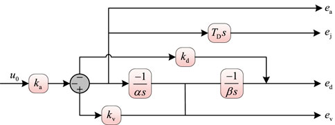
Figure 2. Multi-parameter generator schematic diagram.

Figure 3

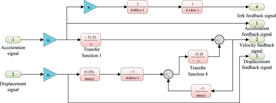
Figure 3. Multi-parameter speed synthesizer simulation model.

In Figure 2, $T_D$ represents the differential time constant, $k_a$、 $k_v$、 $k_d$ represents the acceleration, velocity, and displacement feedback gain in the multi-parameter generator, and $\alpha$ and $\beta$ represent the integral gain.

After applying the multi-parameter control scheme to the two-array system, if G₄ represents the multi-parameter generator transfer function and G₅ represents the multi-parameter feedback transfer function, then the control inputs of the two sub-stations can be written as:

$\left\{\begin{array}{l}{E}_1=G_4{u}_1-G_5{x}_1\\ E_2=G_4{u}_2-G_5{x}_2\end{array}\right.(9)$

Substituting Equation 9 into Equation 8, and further considering the characteristics of the sensors and servo valves, we obtain the control system model. Ultimately, the two-array system model under multi-parameters is obtained Equation 10 as follows:

$\left\{\begin{array}{l}{s}^2{x}_1=\frac{k_{\mathrm{q}}}{A_{\mathrm{p}}}{G}_q{G}_4\frac{\left(G_{\mathrm{p}}{G}_{\text{fa}}{s}^2-G_1{G}_{\mathrm{p}1}^2\right)u_1+G_1{G}_{\mathrm{p}1}^2{u}_2}{G_{\mathrm{p}}{G_{\text{fa}}}^2{s}^2-2G_1{G}_{\mathrm{p}1}^2{G}_{\text{fa}}}\\ s^2{x}_2=\frac{k_{\mathrm{q}}}{A_{\mathrm{p}}}{G}_q{G}_4\frac{\left(G_{\mathrm{p}}{G}_{\text{fa}}{s}^2-G_1{G}_{\mathrm{p}1}^2\right)u_2+G_1{G}_{\mathrm{p}1}^2{u}_1}{G_{\mathrm{p}}{G_{\text{fa}}}^2{s}^2-2G_1{G}_{\mathrm{p}1}^2{G}_{\text{fa}}}\end{array}\right.(10)$

Where Equation 11 is:

$\left\{\begin{array}{l}{G}_{\mathrm{p}}=M_{\mathrm{s}}{s}^2+2cs+2k\\ G_{\mathrm{p}1}=cs+k\\ G_{\mathrm{f}}=G_1\left(M_{\mathrm{t}}{s}^2+cs+k\right)+s+\frac{k_{\mathrm{q}}}{A_{\mathrm{p}}}{G}_5\\ G_{fa}=\frac{1}{s^2}{G}_f\end{array}\right.(11)$

Assume Equation 12 is:

$\left\{\begin{array}{l}{G}_{11}=G_{22}=\frac{k_{\mathrm{q}}}{A_{\mathrm{p}}}{G}_{\mathrm{q}}{G}_4\frac{\left(G_{\mathrm{p}}{G}_{\text{fa}}{s}^2-G_1{G}_{\mathrm{p}1}^2\right)}{G_{\mathrm{p}}{G_{\text{fa}}}^2{s}^2-2G_1{G}_{\mathrm{p}1}^2{G}_{\text{fa}}}\\ G_{12}=G_{21}=\frac{k_{\mathrm{q}}}{A_{\mathrm{p}}}{G}_{\mathrm{q}}{G}_4\frac{G_1{G}_{\mathrm{p}1}^2}{G_{\mathrm{p}}{G_{\text{fa}}}^2{s}^2-2G_1{G}_{\mathrm{p}1}^2{G}_{\text{fa}}}\end{array}\right.(12)$

Write it in the form of a matrix like Equation 13:

$\left\{\begin{array}{l}{s}^2{x}_1\\ s^2{x}_2\end{array}\right\}=\left\{\begin{array}{l}{G}_{11}\\ G_{21}\end{array}\right.\left.\begin{array}{l}{G}_{12}\\ G_{22}\end{array}\right\}\left\{\begin{array}{l}{u}_1\\ u_2\end{array}\right\}(13)$

where: G₁₁ is the transfer function of the input signal of shaker 1 to the acceleration $s^2{x}_1$ of shaker 1, G₁₂ is the transfer function of the input signal of shaker 2 to the acceleration $s^2{x}_1$ of shaker 1; G₂₁ is the transfer function of the input signal of shaker 1 to the acceleration $s^2{x}_2$ of shaker 2, G₂₂ is the transfer function from the input signal of Shaker 2 to the acceleration $s^2{x}_2$ of Shaker 2.

The basic parameters of the hydraulic and control system of the two-array seismic simulation shaker are shown in Supplementary Table 1, and the relevant parameters of the shaker table are also listed.

3 LSTM neural network system identification principle

3.1 Principles and steps of system identification

The principle of system identification is based on the analysis of system input and output data, with the aim of inferring the intrinsic structure and parameters of the system from this data. Using the Controlled Auto-Regressive (CAR) model as an example, the basic principle of system identification can be explained.

Typically, a single-input single-output CAR model can be represented as Equation 14:

$A\left(z^{-1}\right)y\left(k\right)=z^{-d}B\left(z^{-1}\right)u\left(k\right)+\xi \left(k\right)(14)$

where, $y\left(k\right)$ is the system output, $u\left(k\right)$ is the system input, $\xi \left(k\right)$ is a random disturbance, d is pure delay, $A\left(z^{-1}\right)$ and $B\left(z^{-1}\right)$ can be expressed as Equation 15:

$\left\{\begin{array}{l}A\left(z^{-1}\right)=1+a_1{z}^{-1}+a_2{z}^{-2}+\dots +a_p{z}^{-p}\\ B\left(z^{-1}\right)=1+b_1{z}^{-1}+b_2{z}^{-2}+\dots +b_q{z}^{-q}\end{array}\right.(15)$

The model structure of the system is shown in Figure 4, which assumes without loss of generality that $C\left(z^{-1}\right)=1$.

Figure 4

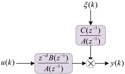
Figure 4. Single input single output CAR model.

Furthermore, the above equation can be written as Equation 16:

$y\left(k\right)={\phi }^T\left(k\right)\theta +\xi \left(k\right)(16)$

where, $\varphi \left(k\right)={\left[-y\left(k-1\right),\dots ,-y\left(k-p\right),u\left(k-d\right),\dots ,u\left(k-d-q\right)\right]}^T$ is a vector constructed from input and output observations, and $\theta ={\left[a_0,\dots ,a_p,b_0,\dots ,b_q\right]}^T$ is the parameter vector to be solved.

During the experiment, by collecting the input and output data of the system, the input data is the control input signal, and the output data is the system’s response signal, that is, obtaining vector $\varphi \left(k\right)$. For systems that can be modeled, such as the CAR model, the system identification problem can be transformed into a parameter estimation problem, that is, finding the optimal parameter $\theta$ estimate by minimizing the error between the model’s predicted values and the actual output.

System identification generally includes the following stages:

(1) Experimental Design: According to different practical requirements, clarify the purpose of model identification, determine the object of system identification, select appropriate input signals, and collect output response data. Generally, suitable input signals should have a certain spectrum and energy distribution to cover the key characteristics of the system and maintain its stability. Moreover, for nonlinear systems, random signals are usually more suitable because they have better excitation performance. The quality of the experimental design directly affects the accuracy of the subsequent model.

(2) Data Collection and Preprocessing: Conduct experiments and collect the input and output data of the system. This includes recording the responses measured by sensors and generating control input signals. Ensure that the experimental environment and measurement errors are considered during data collection. Additionally, preprocess the collected data by performing operations such as denoising, filtering, and sampling to improve the quality and identifiability of the data.

(3) Establish a mathematical model: Use the collected data to create a mathematical model of the system, such as in the form of difference equations, state-space equations, or transfer functions, and estimate the model parameters.

(4) Parameter identification: This typically involves fitting techniques, such as the least squares method, to minimize the error between the model’s predictions and the actual observations.

(5) Model validation and optimization: Use data not involved in the identification process for new tests to verify the accuracy and reliability of the obtained model. Ensure that the model can correctly predict the system’s response under new input conditions. Additionally, analyze the obtained model to understand the dynamic characteristics of the system. Optimize the model as needed to enhance its performance and adaptability.

3.2 LSTM frame structure and model building

LSTM is a special type of neural network structure that is designed to address the problems of gradient vanishing and gradient explosion encountered by traditional neural networks when handling long-term dependencies. The LSTM unit consists of a cell state and three gating components (input gate, forget gate, and output gate). The forget gate is used to determine which information should be discarded from the cell state; the input gate controls the extent to which the current input affects the cell state; and the output gate decides how the cell state influences the next layer. In the context of controlling a seismic simulation shaking table, the aim is to reproduce the input earthquake waves as accurately as possible, with a one-to-one correspondence between input and output. Therefore, a one-to-one LSTM model was ultimately chosen as the controller for the shaking table in this study. The LSTM structure diagram is presented in Figure 5.

Figure 5

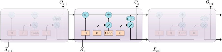
Figure 5. LSTM structure diagram.

In the establishment of the LSTM model, data processing is first conducted to standardize the input seismic wave data to fit the LSTM input format. The dataset is then divided into training and testing sets. Due to the dynamic computation graph utilized in PyTorch, a more intuitive and flexible approach is enabled during the model construction and debugging process. Additionally, the simple and intuitive APIs provided by PyTorch make the construction, training, and evaluation of deep learning models easier. Therefore, the PyTorch framework is employed in this study. In the LSTM used in this research, the model structure is defined using the Sigmoid activation function. The Sigmoid function can independently control the opening and closing states of each gate and possess good gradient propagation characteristics, effectively preventing the problem of gradient vanishing during the training process, thereby achieving selective information transfer.

Then, the Mean Squared Error (MSE) loss function is chosen, and the Adam optimizer is used for backpropagation gradient optimization in this paper. The expression for the MSE loss function is as follows Equation 17:

$MSE=\frac{1}{m}{\displaystyle \sum _{i=1}^m}{\left(y_i-f\left(x_i\right)\right)}^2(17)$

From the above equation, it can be seen that the loss function MSE represents the sum of the squared differences between the predicted value $f\left(x\right)$ of the model and the true value y of the sample. The smaller its value, the smaller the error and the higher the accuracy.

Finally, the input seismic wave dataset is used for model training, and the testing set is employed to evaluate the model’s generalization capability. At the same time, the performance of this approach is assessed using the correlation between the actual results and the predicted results, as well as the root mean square error.

Based on the above, the algorithm flowchart for identifying LSTM network is shown in Figure 6:

Figure 6

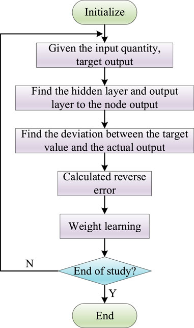
Figure 6. LSTM network identification flowchart.

4 Identification results and analysis of the LSTM dual-array closed-loop system

The LSTM network structure used in this paper specifically includes: an input layer, a hidden layer with 15 neurons, and an output layer. The momentum factor is set to 0.0005, the initial weights of the network are randomly chosen within the range [−1,1], and the learning algorithm employed is the “gradient descent algorithm.” The maximum number of training iterations is set to 20,000, and the loss function is calculated using the MSE formula. The training process for system identification is conducted offline. In the results presented below, the curve labeled “Actual Result” represents the output of the shaking table, which serves as the network’s label. The curve labeled “Forecast Result” represents the output of the neural network. The smaller the deviation between the forecast results and the actual results, the better the training performance of the neural network and the higher the accuracy of the system identification. We will first present intuitive result display graphs, and finally evaluate the performance of this method for system identification using the similarity between the actual and forecast waveforms. Assuming the two waveforms are denoted as x and y, their correlation coefficient can be expressed as Equation 18:

$corr\left(x,y\right)=\frac{{\displaystyle \sum _{n=1}^N}\left(x_n-\overline{x}\right)\left(y_n-\overline{y}\right)}{\sqrt{{\displaystyle \sum _{n=1}^N}{\left(x_n-\overline{x}\right)}^2{\displaystyle \sum _{n=1}^N}{\left(y_n-\overline{y}\right)}^2}}(18)$

We used different seismic waves as input waveforms, with a sampling time of 0.02 s, corresponding to a sampling frequency of 50 Hz. The simulation time is set to 40 s, resulting in two input datasets each containing 4,000 data points. The first 2000 data points are used as the training set, and the remaining 2000 data points are used as the test set. For the dual-array system, the output data is modeled as a two-dimensional matrix, corresponding to the response waveforms of Shaking Table 1 and Shaking Table 2, respectively. We obtained the output of the dual-array closed-loop system through simulation, which serves as the labels for neural network training. Using the EL Centro wave to analyze the training set, the training results of the dual-array closed-loop system are shown in Figure 7.

Figure 7

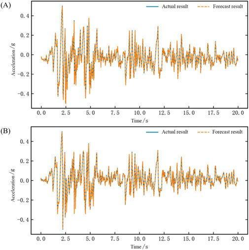
Figure 7. Time domain waveform chart of network training for the dual-array system identification (A) Shaking table 1 training results comparison (B) Shaking table 2 training results comparison.

Figures 7A, B are comparison charts of the output waveforms and network training results for Shaking Table 1 and Table 2, respectively. After calculation, the root mean square error (RMSE) between the network output waveform and the actual waveform is −52.9 dB for Table 1 and -52.8 dB for Table 2. The correlation coefficients are 0.9998 for Table 1 and 0.9998 for Table 2. The network training results match the actual results very well.

For the test set, we used three different seismic waves and one artificial wave for analysis, performing both time domain and frequency domain analyses. First, we analyzed the EL Centro wave, with the time domain chart shown in Figure 8.

Figure 8

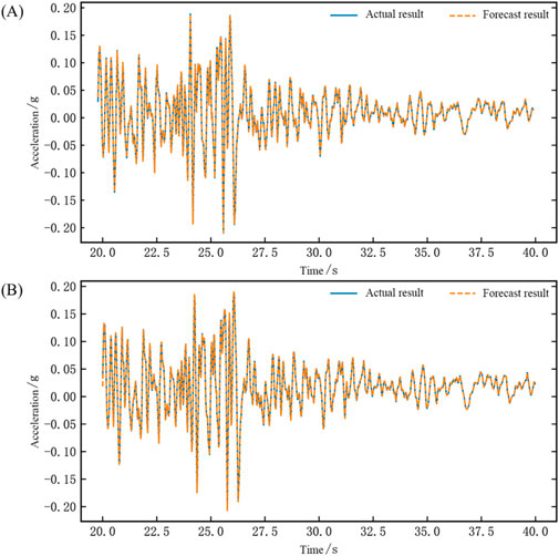
Figure 8. Time domain waveform chart of network testing for the dual-array system identification (EL Centro wave) (A) Comparison chart of results for Shaking Table 1 (B) Comparison chart of results for Shaking Table 2.

The calculated root mean square error (RMSE) between the network output waveform and the actual waveform is −60.4 dB for Table 1 and -60.9 dB for Table 2. The correlation coefficients are 0.9998 for Table 1 and 0.9998 for Table 2. After performing a Fourier transform on the waveform data, the frequency spectrum characteristics of the seismic wave can be obtained, as shown in Figure 9. It can be seen that the frequency domain performance of the network output waveform also almost perfectly replicates the actual frequency domain waveform.

Figure 9

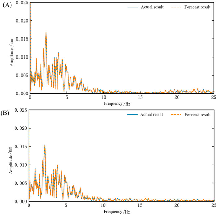
Figure 9. Frequency domain waveform chart of network testing for the dual-array system identification (EL Centro wave) (A) Comparison chart of results for Shaking Table 1 (B) Comparison chart of results for Shaking Table 2.

Next, we performed time and frequency domain analyses of the Wenchuan surface wave, as shown in Figures 10, 11. The calculated results indicate that the root mean square error (RMSE) between the network output waveform and the actual waveform is −42.3 dB for Table 1 and -56.2 dB for Table 2. The correlation coefficients are 0.9996 for Table 1 and 0.9997 for Table 2.

Figure 10

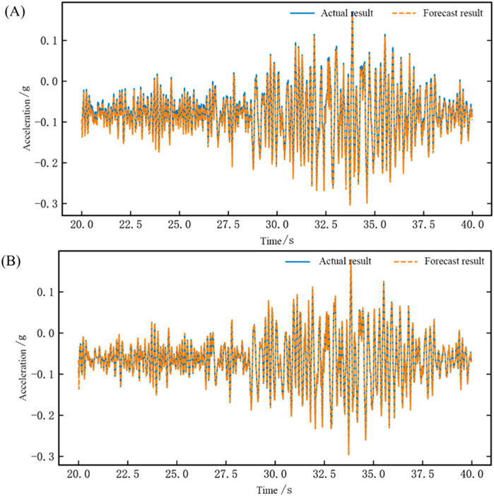
Figure 10. Time domain waveform chart of network testing for the dual-array system identification (Wenchuan floor wave) (A) Comparison chart of results for Shaking Table 1 (B) Comparison chart of results for Shaking Table 2.

Figure 11

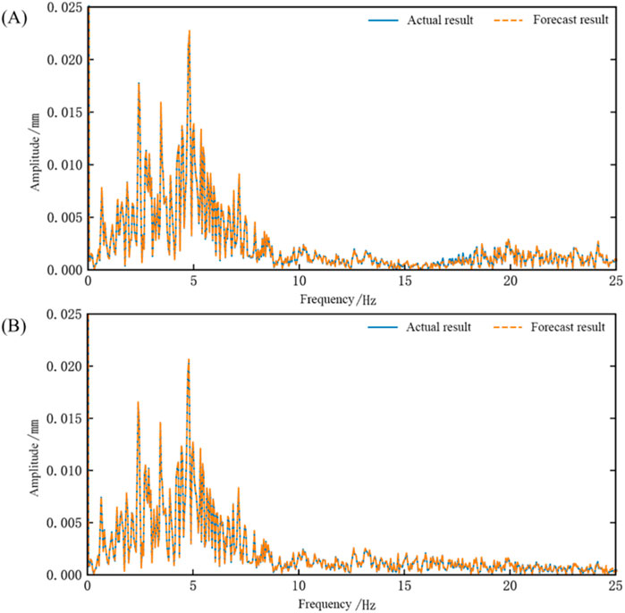
Figure 11. Frequency domain waveform chart of network testing for the dual-array system identification (Wenchuan floor wave) (A) Comparison chart of results for Shaking Table 1 (B) Comparison chart of results for Shaking Table 2.

Next, we performed time and frequency domain analyses using the Traf wave, as shown in Figures 12, 13. The calculated results indicate that the root mean square error (RMSE) between the network output waveform and the actual waveform is −51.74 dB for Table 1 and -51.20 dB for Table 2. The correlation coefficients are 0.9988 for Table 1 and 0.9986 for Table 2.

Figure 12

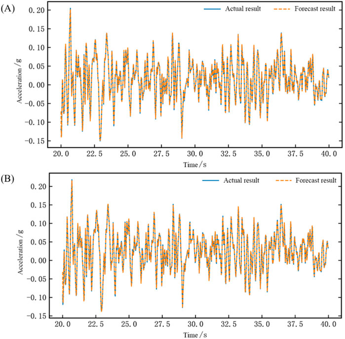
Figure 12. Time domain waveform chart of network testing for the dual-array system identification (Traf wave) (A) Comparison chart of results for Shaking Table 1 (B) Comparison chart of results for Shaking Table 2.

Figure 13

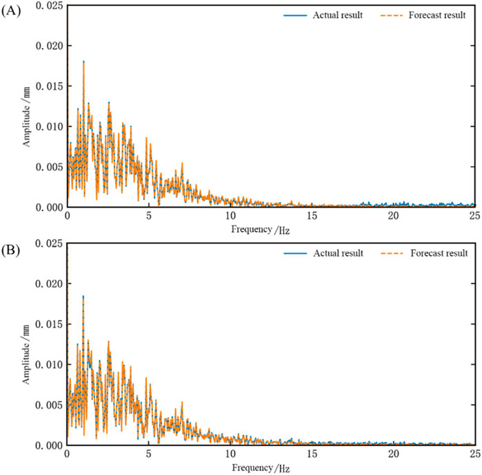
Figure 13. Frequency domain waveform chart of network testing for the dual-array system identification (Traf wave) (A) Comparison chart of results for Shaking Table 1 (B) Comparison chart of results for Shaking Table 2.

Finally, we performed time and frequency domain analyses using the artificial wave, as shown in Figures 14, 15. The calculated results indicate that the root mean square error (RMSE) between the network output waveform and the actual waveform is −49.62 dB for Table 1 and -49.43 dB for Table 2. The correlation coefficients are 0.9996 for Table 1 and 0.9996 for Table 2.

Figure 14

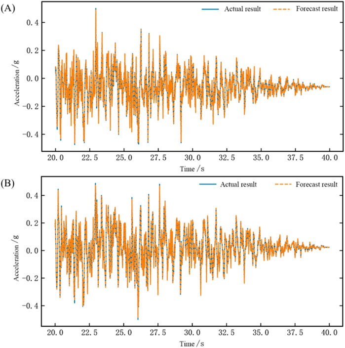
Figure 14. Time domain waveform chart of network testing for the dual-array system identification (Artificial wave) (A) Comparison chart of results for Shaking Table 1 (B) Comparison chart of results for Shaking Table 2.

Figure 15

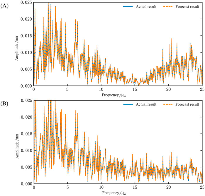
Figure 15. Frequency domain waveform chart of network testing for the dual-array system identification (Artificial wave) (A) Comparison chart of results for Shaking Table 1 (B) Comparison chart of results for Shaking Table 2.

Based on the analysis of these four waveforms, the root mean square error (RMSE) and correlation coefficients between the network output waveforms and the actual time domain waveforms are summarized in Supplementary Table 2. Both the time domain and frequency domain waveform correlations exceed 0.99, indicating that the output closely matches the actual waveforms. This demonstrates that the identification scheme has excellent performance, and the network trained with LSTM can achieve the dual-array system identification task with high accuracy.

5 Conclusion and discussion

This paper primarily designs an identification scheme for a dual-array closed-loop system based on an LSTM network. First, the dual-array system of a seismic simulation shaking table is modeled. Then, a dual-array system identification method based on LSTM is proposed. Using the dataset from the constructed Simulink simulation model, the neural network is trained and tested. The LSTM network is modified to adapt to the system output, considering the characteristics of the dual-array system. This identification scheme is highly applicable, efficient in terms of parameters, and reflects the true characteristics of the system. The main conclusions drawn are as follows:

(1) In training the neural network model, the gradient descent algorithm is highly efficient and adaptable. It effectively handles the nonlinear problems in seismic simulation shaking tables and has broad application prospects in optimizing control systems.

(2) After identification using the LSTM neural network, the output of the seismic simulation shaking table dual-array closely matches the theoretical output, with a low mean square error and a waveform correlation coefficient exceeding 0.99. This verifies that the identification scheme has high accuracy and good convergence, providing a theoretical basis for performance control of the seismic simulation shaking table.

The research work in this paper is based on closed-loop system and single-degree-of-freedom structure. The subsequent research may consider verifying the applicability of the proposed LSTM neural network identification to open-loop system and multi-degree-of-freedom structure, and further improve the efficiency and accuracy of system identification by combining with other intelligent control algorithms.

Data availability statement

The original contributions presented in the study are included in the article/Supplementary Material, further inquiries can be directed to the corresponding author.

Author contributions

CG: Writing–original draft, Writing–review and editing. MW: Writing–review and editing, Writing–original draft. YS: Writing–review and editing. ZY: Writing–review and editing.

Funding

The author(s) declare that financial support was received for the research, authorship, and/or publication of this article. This work was supported by the Henan Provincial Department of Science and Technology (No.212300410234) and Xinyang Normal University (No. 2024KYJJ110).

Acknowledgments

The author thanks the teachers and classmates of the team for collecting the experimental data.

Conflict of interest

The authors declare that the research was conducted in the absence of any commercial or financial relationships that could be construed as a potential conflict of interest.

Publisher’s note

All claims expressed in this article are solely those of the authors and do not necessarily represent those of their affiliated organizations, or those of the publisher, the editors and the reviewers. Any product that may be evaluated in this article, or claim that may be made by its manufacturer, is not guaranteed or endorsed by the publisher.

Supplementary material

The Supplementary Material for this article can be found online at: https://www.frontiersin.org/articles/10.3389/fphy.2024.1475622/full#supplementary-material

References

1. Li P, Liu S, Lu Z, Yang J. Numerical analysis of a shaking table test on dynamic structure-soil-structure interaction under earthquake excitations. The Struct Des Tall Spec Buildings (2017) 26:e1382. doi:10.1002/tal.1382

CrossRef Full Text | Google Scholar

2. Wang S, Gao R, Zhai H, Pang J. Research on synchronous motion control of three shaking tables platform based on EtherCAT. Machinery Des and Manufacture (2018) 168–71+176. doi:10.19356/j.cnki.1001-3997.2018.12.042

CrossRef Full Text | Google Scholar

3. Gao C, Yang Y, Wang J, Qin M, Yuan X. Development and application of a shaking table system. Arab J Geosci (2022) 15:1334. doi:10.1007/s12517-022-10604-6

CrossRef Full Text | Google Scholar

4. Ji J, Li X, Yan W, Li Z, Li H, Cui P, et al. Research on the shaking table array and dynamic model test. Struct Eng (2011) 27:31–6. doi:10.15935/j.cnki.jggcs.2011.s1.007

CrossRef Full Text | Google Scholar

5. Ji J, Li F, Li Z, Sun L. Research and advances on the control technology of the multiple shaking table array system. Struct Eng (2012) 28:96–101. doi:10.15935/j.cnki.jggcs.2012.06.024

CrossRef Full Text | Google Scholar

6. Tao D, Song J, Liu Y, Su Q. Dynamic analysis of double array earthguake simulation shaking table foundation. Building Sci (2016) 32:34–8. doi:10.13614/j.cnki.11-1962/tu.2016.11.007

CrossRef Full Text | Google Scholar

7. Guan G, Xiong W, Wang H. Control of a dual shaking tables vibration test system. J Of Vibration And Shock (2017) 36:207–11+217. doi:10.13465/j.cnki.jvs.2017.06.032

CrossRef Full Text | Google Scholar

8. Enokida R, Ikago K, Guo J, Kajiwara K. Nonlinear signal-based control for shake table experiments with sliding masses. Earthquake Eng and Struct Dyn (2023) 52:1908–31. doi:10.1002/eqe.3852

CrossRef Full Text | Google Scholar

9. Gao C, Li C, Yuan Z, Sima Y, Wang M. Influence and compensation of connection characteristics on shaking table control performance. Sci Rep (2024) 14:6860. doi:10.1038/s41598-024-57239-z

PubMed Abstract | CrossRef Full Text | Google Scholar

10. Zhang X, Wang J. Mechanism study on the interaction effects of shaking table array-test structure. J Low Frequency Noise, Vibration Active Control (2024) 43(0):1424–36. doi:10.1177/14613484241259853

CrossRef Full Text | Google Scholar

11. Wang J, Sun P, Chen L, Yang J, Liu Z, Lian H. Recent advances of deep learning in geological hazard forecasting. CMES (2023) 137:1381–418. doi:10.32604/cmes.2023.023693

CrossRef Full Text | Google Scholar

12. Qu Y, Zhou Z, Chen L, Lian H, Li X, Hu Z, et al. Uncertainty quantification of vibro-acoustic coupling problems for robotic manta ray models based on deep learning. Ocean Eng (2024) 299:117388. doi:10.1016/j.oceaneng.2024.117388

CrossRef Full Text | Google Scholar

13. Chen L, Cheng R, Li S, Lian H, Zheng C, Bordas SPA. A sample-efficient deep learning method for multivariate uncertainty qualification of acoustic–vibration interaction problems. Computer Methods Appl Mech Eng (2022) 393:114784. doi:10.1016/j.cma.2022.114784

CrossRef Full Text | Google Scholar

14. Gao C, Wang J, Yang Y, Qin M. Parameter optimization of shaking table based on later random and nonlinear dynamic particle swarm optimization. J Xinyang Normal Univ (Natural Sci Edition) (2023) 36:137–43. doi:10.3969/j.issn.1003-0972.2023.01.023

CrossRef Full Text | Google Scholar

15. Gao C, Li C, Qin M, Yang Y, Yuan Z. Multi-parameter identification of earthquake simulation shaking table based on BP neural network. Front Phys (2024) 12. doi:10.3389/fphy.2024.1309029

PubMed Abstract | CrossRef Full Text | Google Scholar

16. Yu S, Liu X, Wang J, Liu D, Jin Y. Application of BP neural networks in electro-hydraulic shaking table control system. Chin Hydraulics and Pneumatics (2008) 53–5. doi:10.3969/j.issn.1000-4858.2008.07.020

CrossRef Full Text | Google Scholar

17. Oh BK, Glisic B, Park SW, Park HS. Neural network-based seismic response prediction model for building structures using artificial earthquakes. J Sound Vibration (2020) 468:115109. doi:10.1016/j.jsv.2019.115109

CrossRef Full Text | Google Scholar

18. Zeroual A, Fourar A, Djeddou M. Predictive modeling of static and seismic stability of small homogeneous earth dams using artificial neural network. Arab J Geosci (2019) 12:16. doi:10.1007/s12517-018-4162-6

CrossRef Full Text | Google Scholar

19. Ji J, Hu Z, Yang S. Closed-loop control method of seismic simulation shaking table based on LSTM. EARTHQUAKE ENGINEERING AND ENGINEERING DYNAMICS (2022) 42:63–9. doi:10.13197/j.eeed.2022.0507

CrossRef Full Text | Google Scholar

20. Zhang W, Ji J, Wang D. Parameters tuning of shaking table based on LSTM. Machine Tool And HydraulicS (2024) 52:124–30. doi:10.3969/j.issn.1001-3881.2024.05.019

CrossRef Full Text | Google Scholar

21. Zhang R, Chen Z, Chen S, Zheng J, Büyüköztürk O, Sun H. Deep long short-term memory networks for nonlinear structural seismic response prediction. Computers and Structures (2019) 220:55–68. doi:10.1016/j.compstruc.2019.05.006

CrossRef Full Text | Google Scholar

22. Zhang B, Du H, Zhu F, Wu Y, Rao J, Qiu L. Research on control strategy of random waveform reproduction for single DOF shaking table. Machine Tool and Hydraulics (2023) 51:80–5. doi:10.3969/j.issn.1001-3881.2023.23.012

CrossRef Full Text | Google Scholar

23. Gao C, Yang Y, Qin M, Li C, Yuan Z. Research on parameter identification of shaking table systems based on the RLS method. PLOS ONE (2022) 17:e0279092. doi:10.1371/journal.pone.0279092

PubMed Abstract | CrossRef Full Text | Google Scholar

24. Zhan P, Ji J, Sun L, Wang J, Song L. Research on least souares identification method of shaking table systems. Industrial Construction (2014) 44:285–8+301. doi:10.13204/j.gyjz2014.s1.098

CrossRef Full Text | Google Scholar

25. Ji J, Li W, Wu J. System identification and LSTM network simulation of shaking table open-loop model. Earthquake Engineering and Engineering (2022) 42:87–94. doi:10.13197/j.eeed.2022.0309

CrossRef Full Text | Google Scholar

26. Christudas F, Dhanraj AV. System identification using long short term memory recurrent neural networks for real time conical tank system. Romanian Journal Of Information Science And Technology (2020) 23:T57–T77. doi:10.1016/j.jprocont.2020.10.011

CrossRef Full Text | Google Scholar

27. Guo W, He C, Shao P. A novel system identification method for servo-hydraulic shaking table using physics-guided long short-term memory network. Mechanical Systems and Signal Processing (2022) 178:109277. doi:10.1016/j.ymssp.2022.109277

CrossRef Full Text | Google Scholar