The irreversibility of microscopic motions

People have long had a problem: the equations of motion that reflect the laws of physics are invariant under time inversion, while there always are irreversible processes for gases composed of microscopic particles. This article solves the problem. The point is that we should distinguish between the concepts of the equation of motion and concrete motion. We also need to distinguish between the concepts of time-inverse motion and reverse motion. The former is anticlockwise, which is a fictional motion, while the latter is clockwise. For the single-particle motions in classical mechanics and in quantum mechanics, we present mathematical expressions for time-inversion motion and reverse motion, respectively. We demonstrate that single-particle motion is irreversible. The definition of the reversibility of two-particle collisions is given. According to the definition, the two-particle collision as a microscopic motion process is irreversible. Consequently, for a gas consisting of a large number of particles colliding with each other, its movement should be irreversible, unless the condition of detailed balance is met. We provide a physical explanation for detailed balance, which does not concern the meaning of microscopic reversibility. The detailed balance means that after a pair of reciprocal collisions occur, the distribution function of the particles remains unchanged. Therefore, microscopic two-particle collision events are irreversible, but the statistical average of a large number of collision events makes it possible for the macroscopic process of a gas to be reversible. Conclusively, we clarify the microscopic mechanism of the irreversible process of gases.

1 Introduction

1.1 The paradox of irreversibility

The motion of individual microscopic particles follows the laws of physics. The laws of physics are embodied in equations of motion, which are expressed as differential equations with a derivative with respect to time. It is believed that the equations of motion are time-reversible.

A macroscopic gas is made up of a large number of microscopic particles. Since the equation of motion that every microscopic particle follows is time-reversible, it is thought that macroscopic processes should be reversible either. However, we always observe that irreversible processes occur. Therefore, people are faced with the fact that the laws of motion of microscopic particles are reversible in time, while the motion of macroscopic systems is irreversible [1–13]. It is also said that the movement of microparticles is symmetric with respect to time, but the movement of macro-systems composed of a large number of microparticles is not [4, 5].

This fact forms a paradox: “Classical mechanics itself is entirely symmetrical with respect to the two directions of time. The equations of mechanics remain unaltered when the time t is replaced by –t; if these equations allow any particular motion, they will therefore allow the reverse motion, in which the mechanical system passes through the same configurations in the reverse order. This symmetry must naturally be preserved in a statistics based on classical mechanics. Hence, if any particular process is possible which is accompanied by an increase in the entropy of a closed macroscopic system, the reverse process must also be possible, in which the entropy of the system decreases.” [14].

We use $\left(p_i,q_i\right)$ to represent the ith generalized coordinate and generalized momentum. They follow Hamilton canonical equations:

${\dot{p}}_i=-\frac{\mathit{\partial }H}{\mathit{\partial }{q}_i},q_i=\frac{\mathit{\partial }H}{\mathit{\partial }{\dot{p}}_i}.(1)$

Now, we make time inversion,

$t\to -t.(2)$

Then, we take the following transformation:

$p_i\to -p_i,q_i\to q_i.(3)$

Then, under the transformation Eqs 2, 3, the forms of Eq. 1 remain unchanged. This is the time-reversal invariance of the equations of motion and was called “the principle of dynamical reversibility” [13]. This seems that the movement of each particle should be time-reversible.

Consider that an isolated ideal gas undergoes a process that increases its entropy. At one moment, let the momentum of all molecules reverse, that is, the transformation of Eqs 2, 3 is taken; then, from this moment on, each molecule still moves according to Eq. 1 in the reverse time direction. That is to say, the whole gas moves in the opposite time direction, i.e., it moves in the direction of decreasing entropy. However, such a process is practically impossible. The second law of thermodynamics negates the possibility of such a process. This argument is known as the Loschmidt paradox [2, 13, 15, 16]. The Loschmidt paradox can be stated quite simply: if all the laws of physics are time-reversal-symmetric, how can one prove a time-asymmetric law like the second “law” of thermodynamics that states that the entropy of the Universe “tends to a maximum” [16].

In quantum mechanics (QM), there is the same paradox: “Time irreversibility is not a problem to be solved, ……Theoretically, in particular in the quantum case, realization of time irreversibility is difficult because the fundamental kinetic equations, including the Schrödinger equation and the Dirac equation, ensure that the dynamics are reversible in time” [17]. Some scholars believed that the microreversibility can be employed to provide a way to obtain the statistical cumulants [18].

Someone believed that there was “no conflict between reversible microscopic laws and irreversible macroscopic behavior” [5]. However, when he addressed this, he did not resolve the Loschmidt paradox.

People admit it is a problem and have been troubled by this paradox for more than 100 years. Various efforts have been devoted to eliminate this problem. These efforts speculate about the cause of the irreversibility of macroscopic processes from microscopic reversibility.

One view is that although every microprocess is reversible, the statistical nature of a large number of microprocesses can lead to irreversibility of macroprocesses. For example, the law of motion of each microparticle is time-symmetrical, but the motion that evolves into a macroscopic gas is a diffusion equation, which is temporally asymmetric [5]. However, it is difficult to transit from microscopic equations of motion to macroscopic equations, and there has been no successful solution so far. “There are many conceptual and technical problems encountered in going from a time-symmetric description of the dynamics of atoms to a time-asymmetric description of the evolution of macroscopic systems. This involves a change from Hamiltonian (or Schrödinger) equations to hydrodynamical ones, e.g., the diffusion equation. The problem of reconciling the latter with the former became a central issue in physics during the last part of the 19th century” [5]. This is because “the microscopic details are usually unreachable, and a full description of the system is impossible” [19].

One view is that the irreversibility of thermodynamic processes arises because the initial state of thermodynamic systems is very special [3, 10]. For example, at the initial moment, the gas is confined to a specific region. This view is untenable. If the macroscopic gas is in another initial state, its motion process is still irreversible. There are many initial states from which the motion of a gas is irreversible.

Some scholars think that there are no real isolated systems, and there are always various perturbations that more or less cause molecules to deviate slightly from their intended trajectories after collision. In this way, after multiple collisions, the molecule completely loses its memory. “In reality, it is impossible to produce a totally isolated system. There are always external perturbations present, such as radiation, sunspots or the variable gravitational influence of the surrounding matter.” Thus, “the system loses its memory of the initial state after only a small number of collisions” [10]. “In the forward direction, the macroscopic time development is stable with respect to perturbations but in the time-reversed direction, it is very unstable.” This reason could not provide satisfactory explanation of the paradox and was opposed by others [9]. As a matter of fact, even without external perturbation, an isolated system also follows the law of entropy increase. For instance, in deriving the Boltzmann H theorem, no external affection is considered.

Some scholars think that walls with specific shapes and sizes have an effect on the state of a gas. It is well known that the irreversibility of thermodynamic processes is practically irrespective to the walls.

Prigogine [20] attempted to give a mechanism of irreversibility, called “cascade mechanism.” He thought that the variation in lower-order correlations leads to higher-order correlations, and the appearance of the higher-order correlation was accompanied by a “directed flow.” That was the mechanism of irreversibility. However, he did not explain why there was no opposite directed flow in the higher-order correlations or why the higher-order correlations were anisotropic.

Based on numerical simulations, it was found that microscopic reversibility can lead to a state of time anisotropy. The corresponding mathematical proof is called the fluctuation theorem [21, 22], and the authors thought that it was the “first step toward understanding how macroscopic irreversibility arises from microscopically time-reversible dynamics.” They addressed that “our new proof of how macroscopic irreversibility arises from time reversible microscopic dynamics is valid for all densities” and “time reversibility of the underlying equations of motion is the key component to proving these theorems” [16].

None of the above explanations correctly explain the irreversibility of thermodynamic processes. These explanations give different physical reasons for one physical problem. We think that if there are different interpretations for a physical phenomenon, and none of them can forcefully overturn the others, then, none of them are correct.

Anyhow, the problem remains, and until 2002, “there has been no real change in the situation” [8].

Loschmidt’s reasoning implicitly assumes that because the equation of motion that microscopic particles obey is time-reversible, the motion of the microscopic particle is necessarily time-reversible. This is also known as micro-reversibility, and this assumption is accepted by almost everyone. The time reversibility of the equations of motion is confirmed by transformations Eqs 2, 3. People presuppose the microreversibility and discuss with this premise the cause of the macroirreversibility. However, it has not been demonstrated whether the micromotion is reversible or not. If the micromotion is irreversible, this will inevitably have some consequences. For example, the absence of microscopic reversibility will lead to asymmetry in the probability currents [23].

In order to solve this paradox, we have to clarify the relevant physical concepts. First, we should distinguish concepts of the equation of motion and specific motion. We must carefully study whether specific microscopic movements are reversible or not. If microscopic motion is irreversible, then it is not surprising that macroscopic motion is irreversible, and the so-called paradox disappears naturally. Second, when talking about the reversibility of specific motion, we must distinguish between reverse motion and time-inverse motion.

1.2 Distinguishing the concepts of reverse motion and time-inverse motion

For the motion of an individual particle and the motion of a system, we define the concepts of reverse motion and time-inverse motion, respectively.

The concepts for an individual particle are as follows.

Let a particle be in a state A at time t₀, called the original initial state. Starting from state A, the particle moves clockwise, passing through a series of intermediate states, and reaches an original final state B at time t₁, where $t_1>t_0$. This process is called the original movement process.

We take state B as a new initial state, called the second initial state. Let us consider the following two processes, referred to as opposite processes.

Time-inverse movement process: Starting from the second initial state at time t₁, the particle moves counterclockwise, in the opposite order, passing through each intermediate state in the original process, and returns to a final state that is just the original initial state A at time t₀. Note that $t_0<t_1$. Such a motion is called the time-inverse motion of the original process. This is a fictional movement because in the real world, time always goes to the future.

Reverse movement process: Starting from the second initial state at time t₁, the particle moves clockwise, in the reverse order, passing through each intermediate state in the original process, and returns to the original initial state A at time $t_1+t_1-t_0=2t_1-t_0$. Such a process is called the reverse-movement process of the original process.

If the particle states are described by momentum, the direction of momentum in the opposite processes should be always opposite to that in the original process.

Suppose that one uses a camera to film the original process, and then plays the video backward, if the reverse process is the same as what the video playback shows, then the original process is said to be reversible. Note that when we play the video backward, the time is playing into the future.

Although both the opposite processes describe the motion from the second initial state to the original initial state, the directions of time evolution are just opposite. The two processes have different mathematical expressions, given in Section 2.

We next consider a macroscopic system composed of a large number of microscopic particles, such as a gas. The process that a macrosystem undergoes is a macroprocess. The gas is in a macroscopic state at every macroscopic moment. We mark a macrostate with a capital letter. There can be many microstates corresponding to a macrostate. We mark a microstate with a lowercase Greek letter. At a certain micromoment, the gas is in a specific microstate α of a macrostate A, denoted by Aα.

At the initial moment $t_0$, the gas is in a macroscopic original initial state A, and one of the specific microscopic original initial states α. Starting from this original state Aα, the gas moves clockwise, passing through a series of intermediate states Bβ, and reaches a final state Cγ at time $t_1$, where $t_1>t_0$, called the microscopic original final state. This process is called the original process.

We take Cγ as a new initial state, called the second initial state. If state Cγ is described by the momentum of the microscopic particles, the momentum direction of every particle should be reversed to obtain the second initial state. We consider the following two opposite processes.

Time-inverse movement process: Starting from the second initial state Cγ at time $t_1$, the system moves counterclockwise, in the opposite order, passing through each intermediate state Bβ in the original process, and returns to the original initial state Aα at the earlier time $t_0$. We can imagine that a video recorder films the original process and then plays the video rewind, although the playback is actually done clockwise. Such a motion is called the time-inverse motion of the original process. This is a fictional movement because in the real world, time always goes to the future.

Reverse movement process: Starting from the second initial state at time $t_1$, the system moves clockwise, in the reverse order, passing through each intermediate macrostate B in the original process, and returns to the macro original initial state A at time $2t_1-t_0$. Such a motion process is called the reverse movement process of the original process. If the reverse process can be realized, the original process is said to be reversible, otherwise irreversible.

In the reverse process, merely the intermediate macrostates in the original process are retrieved in the opposite order without the requirement of the details of the microstates. This kind of reversibility, without resorting to microscopic details, is called reversibility in the macroscopic sense. In the time-inverse process and reverse process, the macrostate at every macro moment should be same, but the microstate can be different.

The reason why we make this distinction between the time-inversion process and the reverse process of a macroscopic system is that when people talk about the inverse process of a macrosystem, they actually mean the reverse process defined here, not the time-inversion process. The features of the reverse process are that it is clockwise and that merely the macroscopic states in the original process are required to retrieve in the opposite order, with no requirement of the details of the microstate. Some examples are given as follows.

An original process is that an ice cube dissolves in a cup of boiling water. Its imagined reverse process is impossible. “It is impossible to prepare a cup of lukewarm water in such a way that, 1 hour later, it will turn into an ice cube floating in boiling water” [24]. First, the imagined reverse process is clockwise. Second, the imagined reverse process is not required to retrieve every intermediate microstate in the original process. It is merely required that every intermediate macrostate is retrieved in the opposite order of the original process.

Evaporation and condensation are processes reverse to each other. “Since evaporation and condensation are in general thermodynamically reversible phenomena, the mechanism of evaporation must be the exact reverse of that of condensation, even down to the smallest detail” [25]. Both the evaporation and condensation processes are in progress clockwise, and in the sense of macrostates instead of microstates, they are mutually reversible processes. One of the processes does not mean a time-inverse process of the other.

People talk about the ideal perpetual motion machine of the second kind. This kind of perpetual motion machine is required to carry out a reversible cycle that is repeated over and over again. In each cycle, there must be a reverse process that goes clockwise. Such a fictional machine always works clockwise. Moreover, people do not consider the details of microscopic states in each cycle.

The envisaged Poincaré recurrences [7, 10, 26, 27] are also clockwise processes.

Spin echo is also a clockwise process. It is regarded as the reverse process of the precession of a spin system [28–30].

A gedanken experiment has been conducted [30]. The original process was that a system evolved clockwise starting from the moment $t=0$ until $t=T$. Then, at the moment $t=T$, the system started carrying out a reverse process until $t=2T$. Therefore, this reverse process was also carried out clockwise.

In the introduction of [16], when “the fundamental property of time reversible dynamics” was mentioned, time was supposed to go from 0 to t and then to 2t. Time went clockwise throughout. Although the authors discussed the reverse process, they did not consider time inversion.

When numerical simulations of colliding particle systems by a computer are carried out, the reverse processes move in the clockwise direction [10, 31–33].

Any actually observable process is clockwise. The time-inverse processes are fictitious.

However, people sometimes confuse reverse motion with time-inverse motion, equating the two kinds of motion. That is to regard a clockwise reverse process as an anticlockwise process. Here are some examples.

Lebowitz [3] envisaged an original motion and its reverse motion by a figure. In that figure, the panels A–C “show athletes on a racetrack. At the first gunshot, they start running”, which was the original process. Then, “at the second, they reverse and run back, ending up again in a line.” The reverse process was shown by the panels D–F in that figure, going clockwise. But the author of [3] wrote the caption of the figure by “Reversing time”.

In Fig. 2.4 of [9], the author took time inversion $\mathit{t}\to -\mathit{t}$ at the moment $t=T$. Nevertheless, the system went on to moment $t=2T$. That is to say, after time was inversed, time still went clockwise just as the original process.

Schwable [10] called the manipulation of $\mathit{v}\to -\mathit{v}$ time reversal, but after the manipulation, the system actually still evolved clockwise, as shown in Fig. 10.6 of that study.

The confusion between clockwise and counterclockwise processes probably comes from the following thinking. If an original process of entropy increase is assumed to reverse, the assumed reverse process is necessarily accompanied by entropy decrease. People equate decreasing entropy with time inversion.

Let us review Loschmidt’s reasoning. First, Eq. 1 is the differential equation that particles’ motion should obey, but Loschmidt treated it as the particles’ motion itself, confusing the concepts of the equation of motion and motion. Second, Loschmidt’s starting point was the time reversal of the equation of motion (Eq. 1). That he carried out the transformation (Eq. 2) meant to discuss the time-inverse motion. However, in reality, time always points to the future. So he confused time-inverse motion with reverse motion. What Loschmidt actually wanted to see was an increase in entropy as the gas moved clockwise since he knew that it was impossible to reverse time in reality. What he expected was that the system would still move clockwise, but he could observe the effect of reversing time. We argue in Subsection 3.2 that the outcome he envisaged is impossible.

The definition of a reversible process of a particle’s motion above only involves the motion itself and does not involve its surrounding environment. When a particle undergoes an original process, its surroundings may also change, say, from an original initial state X to Y. Then, at the end of the reverse process, the external environment should return from the Y state to the original initial state X; that is, all external influences brought by the original process are eliminated. If the influence on the surroundings cannot be eliminated, then the process is still irreversible. The same condition applies to a system. So the conditions for an original process carried out by a system to be reversible are that after the reverse process of the system, not only must the system itself return to the original initial state, but the surroundings must also return to their original initial state.

Section 2 explains that the motion of an individual particle is irreversible. For a classical particle, its reverse motion at least needs us to prepare the initial state. Thus, the surroundings are unable to retrieve the initial state of the original process. For a quantum particle, the motion itself is irreversible.

For macroscopic matter such as gases, we should focus on the collision between particles.

1.3 Collision systems

A macroscopic system is made up of a large number of microscopic particles. We roughly divide macrosystems into two categories. The first category, called collision systems, is that the molecules composing the macrosystem collide with each other, such as ideal gases. Any system that does not belong to the first category is called a non-collisional system.

Non-collisional systems are characterized by finite interactions between the particles that make up the system. The change in momentum caused by interactions between particles is continuous. The spatial coordinates of each particle can also change continuously. Hence, the Liouville equation applies to this category of systems. We provide some examples of non-collisional systems. Harmonic and nonharmonic coupling systems [34–41] are non-collisional ones. Spin systems [28–30] and spin glass [42, 43] also belong to this category.

Another example is a system of one-dimensional identical particles [2, 26, 44], although collisions between the particles can occur. “Since the collisions between the molecules are elastic and the particles indistinguishable, we can allow the colliding molecules to move as if they passed through one another without collision” [44]. In the Liouville equation of this system, the term with the derivative of momentum does not appear. Thus, the momentum distribution does not change with time. Nevertheless, the spatial distribution of the particles can vary, tending to be uniformly distributed with time. This system has essentially the same kinematic characteristics as a collision-free system. Indeed, in discussing the variation of the particle distribution of this system, collisions between particles were not taken into account [2]. Therefore, it is also classified as a collision-free system.

In general, because the non-collisional systems satisfy the Liouville equation, their processes may be reversible, and it is possible to estimate the Poincaré recurrence time [26]. It is likely that the non-collisional systems are not ergodic.

We investigate the collision systems made up of a large number of molecules that frequently collide with each other. Such a system is called a gas. We mean the real molecules such as H and CO, not a hard ball model or any other ideal model. Only isolated systems are considered. For the sake of simplicity, we assume that dimension of a gas is very much larger than that of a molecule in the gas so that every molecule moves as if it is in an infinitely large space, and we do not consider the boundary conditions of its motion. We also assume the case of one-component ideal gases composed of identical particles. Only elastic collisions between particles are considered, regardless of the internal degrees of freedom of the particles. The gas is thin enough such that only two-particle collisions occur.

The macroscopic processes of a gas are generally irreversible, except its quasi-static processes. The microscopic mechanism of the macroscopic motion of a gas must be hidden behind the collisions between particles. Therefore, it is necessary to take a closer look at the two-particle collision and its effects.

Some consequences of collisions between particles were investigated [45]. In a gas, the change in the particle’s momentum is discontinuous due to its collision with other particles. As a result, in the phase space, the trajectory of a phase point is not continuous, and the phase function of the gas is not smooth. Because of this reason, one is actually unable to define a density current for the phase points. Consequently, the Liouville equation does not apply. All discussions based on the Liouville equation and on smooth phase functions are problematic. For example, the BBKGY method [7, 27, 46–56] deriving the Boltzmann equation from the Liouville equation is incorrect. The proof of Poincaré recurrence theorem assumes that the phase function is smooth [27], so the proof procedure is incorrect. We do not negate the Boltzmann equation and Poincaré recurrence theorem themselves. Boltzmann himself obtained the Boltzmann equation in his own way [57], without the need of the BBKGY method. Poincaré recurrence theorem itself may be correct, but a rigorous proof is still desirable.

The present work examines more closely the collision process itself. One more consequence of a collision between particles is that the collision causes a sudden change in momentum, which provides randomness to the final state after the collision. As a result, the microscopic process of collisions between particles is irreversible.

In Section 2, we consider whether single-particle motion is reversible. For clarity, the mathematical expressions for time-inverse motion and reverse motion are presented. The conclusion is that the motion of individual particles is essentially irreversible. Section 3 studies the irreversibility of the two-particle collision processes. We demonstrate that individual microscopic collision events are irreversible. Consequently, macroprocesses are generally irreversible. Nevertheless, when the number of particles in a gas is large enough to meet the condition of detailed balance, the quasi-static processes of a gas can be reversible. Section 4 provides our conclusion.

2 The irreversibility of individual-particle motion

We first distinguish between two concepts: the equation of motion that a particle obeys and the specific motion of the particle. The mathematical expressions corresponding to these two concepts are presented. We have a basic point of view: one physical concept should have a corresponding mathematical expression, and theoretical conclusions should be drawn from rigorous mathematical derivation. Two different concepts are of different mathematical expressions. Discussion of physical concepts cannot be clear without explicit mathematical expression and derivations.

First, the case of classical mechanics is studied. In classical mechanics, a particle can be any object that can be described by a massive point with no geometric size. It can be a microparticle, such as a molecule, or a macro-object. Then, the case of quantum mechanics is studied.

2.1 Distinguishing the equation of motion and specific motion

As mentioned in the Introduction, people imply that time reversibility of equations of motion necessarily leads to time reversibility of the motion of individual microparticles. That is to say, the motion of each particle can be carried out anticlockwise since the form of the equation of motion that the particle obeys remains unchanged under time inversion.

An equation of motion expresses a physical law that must be followed by the movement of particles. The physical laws determine how the physical quantities of a particle, such as the coordinates and momentum, vary with time. Equations of motion usually appear as differential equations. In classical mechanics, the most fundamental one is Newton’s second law. It takes the form of

$\frac{\mathrm{d}}{\mathrm{d}t}\mathit{p}-\mathit{F}=0.(4)$

This equation determines how a particle’s momentum should vary with time when it is subject to force F. Eq. 4 is also the first equation in Eq. 1.

We assume that there is no friction in force F. This equation of motion is considered to be reversible in time or symmetrical with respect to time [7, 9, 16], i.e., under the transformation of Eqs 2, 3, the form of Eq. 4 remains unchanged.

When we talk about the motion of a particle, we mean its specific motion process, simply referred to as motion. In classical mechanics, it refers to the specific expression that shows that with time, how the physical quantities of a particle, such as spatial coordinates, velocity, momentum, and energy, actually vary.

Suppose that the variation in a particle’s momentum with time is known as

$\mathit{p}=\mathit{p}\left(t\right).(5)$

At any moment, the magnitude and direction of the momentum are explicitly known. Let time be inversed, $t\to -t$. Then, if the momentum expressed by Eq. 5 satisfies $-\mathit{p}\left(-t\right)=\mathit{p}\left(t\right)$, we say that this motion is of time-reversal invariance; otherwise, it is not.

Thus, we distinguish between the equation of motion and specific motion. Regarding the change in momentum of classical particles, the mathematical expression of the equation of motion is Eq. 4, while that of a specific motion is Eq. 5. A specific motion process can be illustrated by a picture. For instance, with the specific expression Eq. 5, a schematic diagram of momentum over time can be drawn. Figure 1 is a schematic diagram for two-particle collisions. The differential Eq. 4 cannot be represented graphically. What we actually see is the specific motion of the particle, the process represented by Eq. 5. Although the specific expression Eq. 5 certainly follows the laws of physics, it cannot be directly seen from Eq. 4 itself.

Figure 1

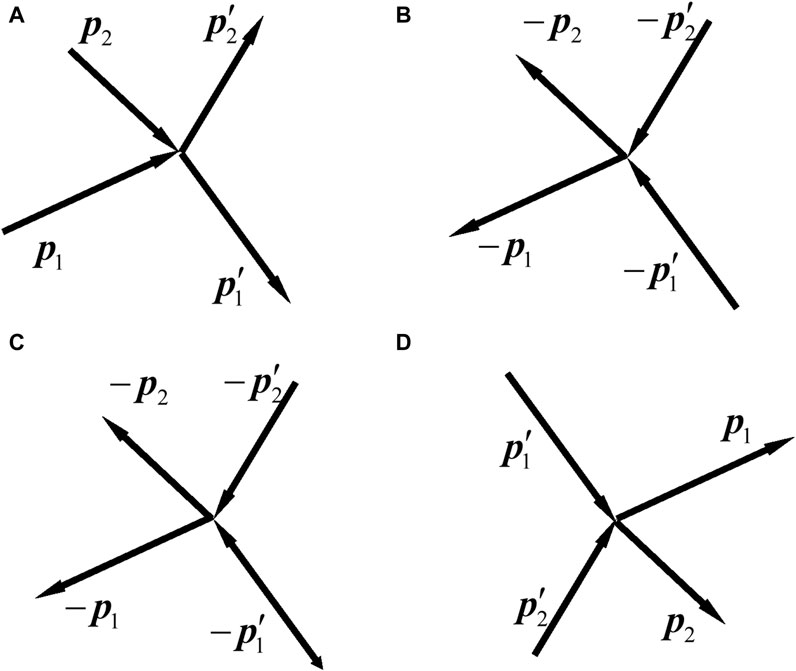
Figure 1. Sketches of the collisions of two free particles. (I) In classical mechanics, a particle with a momentum is represented by a line segment with an arrow. (A) The momenta of the particles before and after the collision are $\left({\mathit{p}}_1,{\mathit{p}}_2\right)$ and $\left({\mathit{p}}_1^{\prime },{\mathit{p}}_2^{\prime }\right)$, respectively. The original collision process is denoted as $\left({\mathit{p}}_1,{\mathit{p}}_2\right)\to \left({\mathit{p}}_1^{\prime },{\mathit{p}}_2^{\prime }\right)$. (B) Time-inverse collision of (A) $\left(-{\mathit{p}}_1^{\prime },-{\mathit{p}}_2^{\prime }\right)\to \left(-{\mathit{p}}_1,-{\mathit{p}}_2\right)$. (C) Reverse collision of (A) $\left(-{\mathit{p}}_1^{\prime },-{\mathit{p}}_2^{\prime }\right)\to \left(-{\mathit{p}}_1,-{\mathit{p}}_2\right)$. (D) Reciprocal collision of (A) $\left({\mathit{p}}_1^{\prime },{\mathit{p}}_2^{\prime }\right)\to \left({\mathit{p}}_1,{\mathit{p}}_2\right)$. (ii) In QM, a plane wave with a momentum is represented by a line segment with an arrow. (A) Scattering of two free particles having plane waves with momenta $\left({\mathit{p}}_1,{\mathit{p}}_2\right)$. After the scattering, the two particles transit to the two plane waves with momenta $\left({\mathit{p}}_1^{\prime },{\mathit{p}}_2^{\prime }\right)$. This original transition process is denoted as $\left({\mathit{p}}_1,{\mathit{p}}_2\right)\to \left({\mathit{p}}_1^{\prime },{\mathit{p}}_2^{\prime }\right)$. (B), (C), and (D) are the time-inverse, reverse, and reciprocal transition processes of (A), respectively. The denotations of (B), (C), and (D) are the same as those in the case of classical mechanics. (B) and (C) look the same, but the former is anticlockwise, and the latter is clockwise. (A) and (D) are clockwise processes.

It is generally implicitly assumed that if the equation of motion Eq. 4 is time-reversible, then, necessarily, Eq. 5 is also temporally reversible. “The equations of classical mechanics are invariant under time reversal. Intuitively, this says that if a film of a sequence of events is run backward, what is seen on the screen appears to be physically possible” [9]. This is equating Eq. 4 and Eq. 5, which reflects that the two concepts, the equation of motion and the motion of particles, are confused.

The irreversibility of movement is occasionally mentioned. It was mentioned [1, 2] that the irreversibility of single-particle motion in an infinitely large system was trivial irreversibility. However, there was no conceptual distinction between motion and equations of motion.

Let a differential equation be integrated in some way so as to obtain the expression of the physical quantity with time. Such a relation is called the general solution of a differential equation. For example, the indefinite integral solution of Eq. 4 results in a general solution:

$\mathit{p}\left(t\right)=\int \mathrm{d}{t}^{\prime }\mathit{F}\left(t^{\prime }\right)+C.(6)$

The process of finding a general solution is a purely mathematical operation without adding any physical factor.

So, does Eq. 6 describe the specific motion of the particle? Or, is it equivalent to Eq. 5. The answer is no. This is because there is a pending constant in Eq. 6, the value of which can only be determined by initial conditions. This constant is set by adding physical factors.

Physically, any specific motion of any particle has a starting point in time. From the Big Bang model, we know that our universe has a time beginning. Therefore, any movement that actually occurs in the universe has a starting point in time. Movement without a starting point of time does not exist. Few studies note that specific motion should have initial conditions [6].

Hereafter, the initial time is denoted as $t_0$. When we mentioned time inversion above, we took $t\to -t$, which defaulted $t_0=0$. As $t_0\ne 0$, time inversion should be expressed as $t-t_0\to -\left(t-t_0\right)$.

Mathematically, differential equations with derivatives with respect to time are always solved under certain initial conditions. For example, the initial condition required to solve Eq. 4 is

$\mathit{p}\left(t=t_0^{+}\right)={\mathit{p}}_0,t_0^{+}=t_0+0^{+}.(7)$

A solution of the equation of motion that meets certain initial conditions is that describing the specific motion; hence, it is called a specific solution. For example, the specific solution of Eq. 4 satisfying the initial condition (Eq. 7) is

$\mathit{p}\left(t\right)={\int }_{t_0}^t\mathrm{d}{t}^{\prime }\mathit{F}\left(t^{\prime }\right)+{\mathit{p}}_0.(8)$

In Eq. 8, the initial condition has already been used, i.e., the pending constant has been determined. Thus, Eq. 8 clearly describes the specific process of movement, which is just Eq. 5 that is required.

As given above, we have tacitly assumed that time evolves clockwise from the initial moment $t_0$. So we talk about the movement in the time range

$t>t_0.(9)$

The possible characteristics of motion can be analyzed from the general solution of the equation of motion (Eq. 6). For example, for a celestial body subject to gravitational action, there is an association between its radial and angular coordinates. The relationship may be elliptical, parabolic, or hyperbolic. When carrying out such a qualitative analysis, the initial condition is not necessary, so it is usually ignored. However, the qualitative analysis does not provide a specific orbit because there is a coefficient called eccentricity to be determined by the initial condition. Therefore, analyzing the specific movement process needs the initial condition.

It is observed that there are actually two elements for describing the motion of a particle: the differential Eq. 4 and the initial conditions and Eq. 7. The physical law (Eq. 4) itself has only differential equations with no initial conditions.

Under different initial conditions, a differential equation may have different specific solutions, i.e., the details of the motion under different conditions may be different, reflecting different specific movement processes. These processes obey the same physical law. For example, imagine an object moving closer to Earth from a distance. When approaching Earth to a certain extent, it may fall to, rotate around, and move away from Earth. These three movements are different, and the one achieved depends on the initial conditions of this object. However, these three possible specific motions follow the same physical law: objects move according to Newton’s second law (Eq. 4) under the gravitational pull of Earth.

Therefore, we clarify that equations of motion (Eq. 4) cannot be equated with specific motion (Eq. 5). The temporal inversion of Eq. 4 does not determine the temporal inversion of the specific motion (Eq. 5).

Only a specific solution (Eq. 8) that meets the initial conditions describes a specific motion. So, is Eq. 8 temporally inverted or reversible? It seems not easy to provide the answer directly from Eq. 8 itself. We carry out a further analysis below.

2.2 The equation of time-retarded motion of a particle

When we talk about the equation of motion (Eq. 4), we are not clear whether time t points to the past or to the future. “The equations of motion in physics are by themselves insufficient to predict what goes on in the Universe. Those equations must be supplemented with the axiom of causality” [16]. The so-called axiom of causality means “Only the past influences the present. The future will, in turn, be influenced by the present. The future cannot influence the present” [16]. There is a close connection between the assumption of causality and the second law of thermodynamics [58].

The initial conditions presented above indicated that time went clockwise.

If a motion is carried out with time going to the future (past), i.e., in the clockwise (anticlockwise) direction, it is called time-retarded (time-advanced) motion, or, in short, retarded (advanced) motion. The function that describes the retarded (advanced) movement is called retarded (advanced) function.

People always talk about retarded motion if there is no additional word. For example, we have implicitly assumed that Eq. 8 described a retarded motion in the time range (Eq. 9). However, the solution to Eq. 8 itself does not explicitly indicate that this is a retarded motion without the supplement of Eq. 9. A physical concept should have its corresponding mathematical expression. The mathematical expression reflecting the time-retarded motion is the time step function $\theta \left(t-t_0\right)$. Few scholars when discussing the scattering theory and path integral in QM noted this point [59–62]. We established the differential equations satisfied by the time-retarded function and time-advanced function [63, 64]. Here, we follow the same idea to establish the differential equations satisfied by the retarded and advanced functions corresponding to Eq. 4.

To explicitly label a retarded motion, we attach a superscript R to the momentum, ${\mathit{p}}^{\mathrm{R}}$, which is called a retarded solution. We think that the differential equation satisfied by the retarded solution ${\mathit{p}}^{\mathrm{R}}$ is

$\frac{\mathrm{d}}{\mathrm{d}t}{\mathit{p}}^{\mathrm{R}}\left(t\right)-\theta \left(t-t_0\right)\mathit{F}=\frac{\partial \theta \left(t-t_0\right)}{\partial t}{\mathit{p}}_0.(10)$

Usually, the derivative of the step function is written as the Dirac delta function, $\frac{\partial \theta \left(t-t_0\right)}{\partial t}=\delta \left(t-t_0\right)$. We stress [63–66] that the rigorous result should be as follows:

$\frac{\partial \theta \left(t-t_0\right)}{\partial t}=\delta \left(t-t_0\right)-\eta \theta \left(t-t_0\right),\eta \to 0^{+}.(11)$

The term with an infinitesimal η should not be discarded. It is because an infinitesimal term cannot be ignored compared to 0. The Dirac delta function itself is invariant with respect to the change in its argument sign, while the time step function is not. Since the function $\theta \left(t-t_0\right)$ reflects time delay, this information should be retained after the derivative with respect to time. The term with the infinitesimal in Eq. 11 reflects the delay in time. A careful discussion of Eq. 11 is given in the appendix of [63].

Equation 10 also indicates that force F acts at time $t>t_0$. Since only the motion in the time range $t>t_0$ is described, the retarded solution ought to have a time delay factor $\theta \left(t-t_0\right)$. We explicitly separate this factor:

${\mathit{p}}^{\mathrm{R}}\left(t\right)=\theta \left(t-t_0\right)\mathit{p}\left(t\right).(12)$

Equation 12 is substituted into Eq. 10.

$\theta \left(t-t_0\right)\left(\frac{\mathrm{d}}{\mathrm{d}t}\mathit{p}\left(t\right)-\mathit{F}\right)=\frac{\partial \theta \left(t-t_0\right)}{\partial t}\left({\mathit{p}}_0-\mathit{p}\left(t\right)\right).(13)$

We let both sides of Eq. 13 be 0. That the left hand side is 0 leads to Eqs 4, 9, and that the right hand side is 0 gives the initial condition (Eq. 7).

Equation 10 is called the equation of retarded motion. It contains both the equation of motion (Eq. 4) and the initial condition (Eq. 7). This form of Eq. 10 is helpful to clearly recognize the physical meaning of retarded motion. It should be noted that Eq. 8 satisfies Eq. 4 and the initial condition (Eq. 7). Nevertheless, what really describes specific movements should be Eq. 12, for the factor $\theta \left(t-t_0\right)$ should not be ignored.

A combination of Eqs 8, 12 results in the solution of Eq. 10 to be

${\mathit{p}}^{\mathrm{R}}\left(t\right)=\theta \left(t-t_0\right)\left({\int }_{t_0}^t\mathrm{d}{t}^{\prime }\mathit{F}+{\mathit{p}}_0\right).(14)$

This form of the solution makes us clearly discuss the reverse process of a specific motion, while Eq. 4 itself does not.

Since there is an infinitesimal term in Eq. 11, the right side of Eq. 10 is not invariant under inversion $t-t_0\to -\left(t-t_0\right)$. Therefore, Eq. 10 describing retarded motion does not guarantee that motion has invariance under time inversion.

In the Introduction, we mentioned that a distinction should be made between the concepts of time-inverse motion and reverse motion. Now, we provide the mathematical expressions for these two concepts.

2.3 The time-advanced motion of a particle

The time-retarded motion above describes the motion in the time range Eq. 9 starting from the initial moment $t_0$. On the contrary, the time-advanced motion describes the motion, starting from the initial moment $t_0$, in the time range

$t<t_0.(15)$

Equation 15 means that the motion goes anticlockwise starting from $t_0$.

The time-advanced motion and aforementioned time-inverse motion, both being counterclockwise, are two concepts, and their corresponding mathematical expressions are different. We present the mathematical expressions.

Usually, when people discuss the time-inversion invariance of the equation of motion, they consider inversion Eq. 2. Then, after the transformations Eqs 2, 3, the equation of motion (Eq. 4) remains unchanged. The time t after the transformation still points to the future, with defaults $t=0$ as the initial moment. Such an approach is not conducive to discussing counterclockwise movement.

We do not take the time inversion (Eq. 2). The equation of motion describing the anticlockwise motion of a particle is

$-\frac{\mathrm{d}}{\mathrm{d}t}\mathit{p}-\mathit{F}=0;t<t_0.(16)$

Here, the momentum is transformed according to Eq. 3. Since we do not take the time inversion (Eq. 2), time t in Eq. 16 moves anticlockwise. The initial moment is set as $t_0$. The form of Eq. 16 is convenient for discussing the anticlockwise motion.

Now, we describe the time-advanced motion in a way similar to that for time-retarded motion described above. We add a superscript A to momentum, ${\mathit{p}}^{\mathrm{A}}$, which is called time-advanced momentum. It obeys the following differential equation:

$\frac{\mathrm{d}}{\mathrm{d}t}{\mathit{p}}^{\mathrm{A}}\left(t\right)+\theta \left(t_0-t\right)\mathit{F}=\frac{\partial \theta \left(t_0-t\right)}{\partial t}{\mathit{p}}_0.(17)$

Naturally, the solution should have the form of

${\mathit{p}}^{\mathrm{A}}\left(t\right)=\theta \left(t_0-t\right)\mathit{p}\left(t\right).(18)$

This is substituted into Eq. 17, and the resultant is

$\theta \left(t_0-t\right)\left(\frac{\mathrm{d}}{\mathrm{d}t}\mathit{p}\left(t\right)+\mathit{F}\right)=\frac{\partial \theta \left(t_0-t\right)}{\partial t}\left({\mathit{p}}_0-\mathit{p}\left(t\right)\right).(19)$

We let both sides of Eq. 19 be 0. When the left hand side is 0, it results in Eq. 16, and when the right hand side is 0, it leads to the initial condition:

$\mathit{p}\left(t=t_0^{-}\right)={\mathit{p}}_0,t_0^{-}=t_0-0^{+}.(20)$

The specific solution satisfying both Eq. 16 and the initial condition (Eq. 20) is

$\mathit{p}\left(t\right)=-{{\displaystyle \int }}_{t_0}^t\mathrm{d}{t}^{\prime }\mathit{F}\left(t^{\prime }\right)+{\mathit{p}}_0.(21)$

The equation of advanced motion (Eq. 17) contains both Eq. 16 and the initial condition (Eq. 20). It is useful for us to discuss counterclockwise movement. We regard the time-inverse motion and counterclockwise motion as synonyms.

Let us examine that a particle first moves clockwise for a period of time and then moves counterclockwise.

When the particle moves clockwise, its momentum varies according to Eq. 14. At the moment $t_1$, its momentum becomes ${\mathit{p}}^{\mathrm{R}}\left(t_1\right)={\mathit{p}}_1$,

${\mathit{p}}_1=\theta \left(t_1-t_0\right)\left({\int }_{t_0}^{t_1}\mathrm{d}{t}^{\prime }\mathit{F}+{\mathit{p}}_0\right).(22)$

After the moment $t_1$, the particle moves anticlockwise, and the initial condition should be $\mathit{p}\left(t_1\right)=-{\mathit{p}}_1$. By Eqs 18, 21, the advanced momentum varies with time as follows:

${\mathit{p}}^{\mathrm{A}}\left(t\right)=\theta \left(t_1-t\right)\left(-{\int }_{t_1}^t\mathrm{d}{t}^{\prime }\mathit{F}-{\mathit{p}}_1\right).(23)$

We substitute Eq. 22 into Eq. 23 and use $\theta \left(t_1-t\right)\theta \left(t_1-t_0\right)=\theta \left(t_1-t\right)$ to obtain

${\mathit{p}}^{\mathrm{A}}\left(t\right)=-\theta \left(t_1-t\right)\left({{\displaystyle \int }}_{t_0}^t\mathrm{d}{t}^{\prime }\mathit{F}+{\mathit{p}}_0\right).(24)$

By comparing Eqs 24, 21, we know that in the time period $t_0\le t\le t_1$, the anticlockwise motion of the particle is strictly the inverse of the clockwise motion. In particular, the momentum at the “final moment $t_0$” of the counterclockwise motion (Eq. 24) is just the negative sign of the momentum of the “initial moment $t_0$” of the clockwise motion (Eq. 21). The condition is that force F is the same at the same moment in the clockwise and counterclockwise time frames.

Therefore, if the initial condition $-{\mathit{p}}_1$ of the advanced motion can be prepared, the integrand F is finite, and the integral can be carried out, this time-advanced process can be achieved, and the particle’s momentum can reach $-{\mathit{p}}_0$. An important postulation is that time can be inversed.

2.4 The reverse motion of a particle

Let us examine the reverse motion of the movement process (Eq. 14). This means that at moment $t_1$, the particle takes the minus sign of Eq. 22, $-{\mathit{p}}_1$, and then moves clockwise. We want to see if it moves in reverse order through each intermediate state of Eq. 14 and finally reaches the minus sign of its initial momentum, $-{\mathit{p}}_0$. This reverse motion is a time-retarded one.

The initial condition of the reverse motion is $\mathit{p}\left(t_1\right)=-{\mathit{p}}_1$. Starting from the moment $t_1$, the particle moves in the way of

${\mathit{p}}^{\mathrm{R}}=\theta \left(t-t_1\right)\left({\int }_{t_1}^t\mathrm{d}{t}^{\prime }\mathit{F}-{\mathit{p}}_1\right)=\theta \left(t-t_1\right)\left({\int }_{t_1}^t\mathrm{d}{t}^{\prime }\mathit{F}-{\int }_{t_0}^{t_1}\mathrm{d}{t}^{\prime }\mathit{F}-{\mathit{p}}_0\right).(25)$

The first integration in Eq. 25 is divided into two parts, ${\int }_{t_1}^t\mathrm{d}{t}^{\prime }={\int }_{2t_1-t}^{t_1}\mathrm{d}{t}^{\prime }+{\int }_{t_0}^{2t_1-t}\mathrm{d}{t}^{\prime }$. Suppose that within the time period $t_1\le t\le 2t_1-t_0$, the force F meets the relationship

$\mathit{F}\left(t\right)=\mathit{F}\left(2t_1-t\right),t_1\le t\le 2t_1-t_0.(26)$

Then, we have

${\int }_{t_1}^t\mathrm{d}{t}^{\prime }\mathit{F}-{{\displaystyle \int }}_{2t_1-t}^{t_1}\mathrm{d}{t}^{\prime }\mathit{F}=0.(27)$

It follows from Eqs 26, 27 that

${\mathit{p}}^{\mathrm{R}}=-\theta \left(t-t_1\right)\left({{\displaystyle \int }}_{t_0}^{2t_1-t}\mathrm{d}{t}^{\prime }\mathit{F}+{\mathit{p}}_0\right).(28)$

Equation 28 demonstrates that in this time period, the momentum changes strictly in reverse order over the time period $t_0\le t\le t_1$. In particular, ${\mathit{p}}^{\mathrm{R}}\left(2t_1-t_0\right)=-\mathit{p}\left(t_0\right)$, which is the minus sign of the original initial momentum $\mathit{p}\left(t_0\right)$.

Thus, the condition that motion Eq. 14 is reversible is that the initial condition (Eq. 22) can be prepared, and the force F satisfies condition Eq. 26 and can be integrated over time.

For example, Earth–Moon is regarded as an isolated two-body system, in which Earth is considered to be static, and the Moon rotates around Earth by gravitational pull. Gravity meets condition Eq. 26. If at a moment the momentum of the moon is reversed, the subsequent motion is the reverse motion. There is a premise that the initial condition of reverse motion can be realized. We know that the initial conditions of reversing the momentum of the Moon are unattainable. So, in reality, this reverse motion is impossible to achieve. The conclusion is that the motion of the Moon around Earth is irreversible.

In general, when discussing an original process (Eq. 14), there is no restriction on its initial condition. We always discuss the motion of a particle when the initial condition (Eq. 7) has been achieved.

By contrast, if we talk about the reverse motion of a known original motion process, its initial condition is not arbitrary, but is determined by the final state of the original motion and needs to be prepared. If the initial condition cannot be prepared, the original motion is irreversible. For example, an original motion is that, in a vacuum, a bullet is fired from the muzzle of a gun and reaches the target. No one can achieve its reverse motion.

If, after the occurrence of the original process (Eq. 14), there is a probability that the initial condition of the reverse process can be realized but the probability is less than 1, we think that the original motion process is still irreversible.

Even if we can prepare an initial condition, the surroundings are inevitably influenced in the course of the preparation. That is to say, the environment cannot return to the original initial state. In this case, we think that the original motion is still irreversible.

It is observed that the conditions for the reversibility of the motion of a particle are quite harsh. We can conclude that in classical mechanics, the motion of a particle is basically irreversible.

2.5 The motion of a particle in quantum mechanics is irreversible

In QM, the motion of microscopic particles with the property of wave–particle duality is described. The fundamental equations of motion, as well as the physical quantities, are different from those in classical mechanics. However, the idea of analyzing the time-inverse motion and reverse motion of a particle is consistent with that for classical mechanics presented above.

A fundamental physical quantity in QM is wave function $\psi \left(\mathit{r},t\right)$. By use of the wave function, we can calculate the expectations of some other physical quantities, such as particle density distributed in space, current density of particles, momentum, kinetic energy, energy, and density of states.

The fundamental equations in QM are differential equations used to solve wave functions, mainly the Schrödinger equation and Dirac equation. They have the following form:

$\left(\mathrm{i}\hslash \frac{\partial }{\partial t}-H\right)\psi \left(\mathit{r},t\right)=0.(29)$

The time inversion (Eq. 2) is taken in Eq. 29, and subsequently, in the transformed equation, the time again points to the future, and the solution becomes ${\psi }^{*}\left(\mathit{r},t\right)$, the complex conjugate of $\psi \left(\mathit{r},t\right)$ [67]. Here, we do not take the time inversion (Eq. 2) but simply retain Eq. 29 unchanged, keeping in mind that the time therein can go anticlockwise. So Eq. 29 stands for both the time-retarded and time-advanced motions.

The dependence of the wave function on time describes the specific motion.

$\psi =\psi \left(\mathit{r},t\right).(30)$

The differential Eq. 29 shows us the fundamental law that a particle’s motion must obey. From Eq. 29 itself, one is unable to see the specific motion described by Eq. 30.

Since the equation of motion (Eq. 29) has time inversion invariance, the specific motion (Eq. 30) of a particle should have either.

We stress that the equation of motion (Eq. 29) and concrete motion (Eq. 30) are two different concepts. Eq. 29 indeed remains unchanged under time inversion, but this does not guarantee that the motion process described by Eq. 30 is reversible.

In order to solve a specific motion from Eq. 29, an initial condition is required.

$\psi \left(\mathit{r},t=t_0^{+}\right)=\psi \left(\mathit{r},t_0^{+}\right).(31)$

A combination of Eqs 29, 31 results in the expression of the specific motion [63, 64]:

$\psi \left(\mathit{r},t\right)=\exp \left(-\frac{\mathrm{i}}{\hslash }{\int }_{t_0}^t\mathrm{d}{t}^{\prime }H\left(t^{\prime }\right)\right)\psi \left(\mathit{r},t_0\right).(32)$

The initial condition has been employed in the solution. Because Eq. 29 is a homogeneous one, the initial condition provides a factor in Eq. 32, instead of an additional term as that in Eq. 8.

If the Hamiltonian H has a complete set of eigenfunctions $\left\{{\phi }_n\left(\mathit{r},t\right)\right\}$, the solution of Eq. 29 can be written as the superposition of this complete set.

$\psi \left(\mathit{r},t\right)={\displaystyle \sum _n}{c}_n{\phi }_n\left(\mathit{r},t\right).(33)$

For example, the Hamiltonian of a free particle is

$H=-\frac{{\hslash }^2}{2m}{\nabla }^2.(34)$

Its complete set of eigenfunctions and corresponding energies are

${\phi }_{\mathit{k}}\left(\mathit{r},t\right)=\frac{1}{{\left(2\mathrm{\pi }\right)}^{3/2}}{\mathrm{e}}^{-\mathrm{i}\left(E\left(\mathit{k}\right)t/\hslash -\mathit{k}\cdot \mathit{r}\right)},E\left(\mathit{k}\right)=\frac{{\hslash }^2{\mathit{k}}^2}{2m}.(35)$

Equation 33 is the general solution of Eq. 29. From the general solution, one can analyze the features the wave function may have, but the real specific movement cannot be certain yet, unless the initial condition is known. When the expansion coefficient in Eq. 33 is determined by the initial conditions, Eq. 33 becomes a specific solution.

Thus, describing a specific motion of a particle requires two elements: the differential Eq. 29 and the initial conditions.

A differential equation can have different solutions subject to different initial conditions. Each specific motion has its own details. For the Hamiltonian (Eq. 34) of a free particle, if the initial condition is a plane wave, the specific solution is a single plane wave. If the initial condition is a wave packet, the particular solution is a traveling while collapsing wave packet.

Solution Eq. 32 does not clearly indicate whether this is a retarded or advanced movement. Usually, it is defaulted that this is a retarded motion.

Now, we explicitly discuss retarded motion, i.e., the motion in time range $t>t_0$ after the initial moment $t_0$. We add a superscript R to the wave function, ${\psi }^{\mathrm{R}}\left(\mathit{r},t\right)$, to mark that this is a time-retarded wave function. The equation of motion satisfied by ${\psi }^{\mathrm{R}}\left(\mathit{r},t\right)$ is

$\left(\mathrm{i}\mathit{\hslash }\frac{\partial }{\partial t}-H\right){\psi }^{\mathrm{R}}\left(\mathit{r},t\right)=\mathrm{i}\hslash \frac{\partial \theta \left(t-t_0\right)}{\partial t}\psi \left(\mathit{r},t_0\right).(36)$

Since ${\psi }^{\mathrm{R}}\left(\mathit{r},t\right)$ is a time-retarded wave function, it is written in the form of

${\psi }^{\mathrm{R}}\left(\mathit{r},t\right)=\theta \left(t-t_0\right)\psi \left(\mathit{r},t\right).(37)$

The factor $\theta \left(t-t_0\right)$ unambiguously indicates that time evolves toward the future [59–62].

After Eq. 37 is substituted into Eq. 36, we obtain

$\theta \left(t-t_0\right)\left(\mathrm{i}\mathit{\hslash }\frac{\partial }{\partial t}-H\right)\psi \left(\mathit{r},t\right)=\mathrm{i}\hslash \frac{\partial \theta \left(t-t_0\right)}{\partial t}\left[\psi \left(\mathit{r},t_0\right)-\psi \left(\mathit{r},t\right)\right].(38)$

We let both sides of Eq. 38 be 0. When the left-hand side is 0, it leads to Eqs 29, 9, and when the right-hand side is 0, it results in the initial condition (Eq. 31). Thus, Eq. 36 contains both the equation of motion and the initial condition.

It follows from the combination of Eq. 32 and Eq. 37 that

${\psi }^{\mathrm{R}}\left(\mathit{r},t\right)=\theta \left(t-t_0\right)\exp \left(-\frac{\mathrm{i}}{\hslash }{\int }_{t_0}^t\mathrm{d}{t}^{\prime }H\left(t^{\prime }\right)\right)\psi \left(\mathit{r},t_0\right).(39)$

Note that the specific solution Eq. 32 satisfies the differential Eq. 29 and the initial condition Eq. 31. However, the solution that really describes the retarded movement should be Eq. 39.

With the preparation above, we discuss the time-inverse motion and reverse motion.

The time-advanced wave function ${\psi }^{\mathrm{A}}\left(\mathit{r},t\right)$ obeys the following equation:

$\left(\mathrm{i}\hslash \frac{\partial }{\partial t}-H\right){\psi }^{\mathrm{A}}\left(\mathit{r},t\right)=\mathrm{i}\hslash \frac{\partial \theta \left(t_0-t\right)}{\partial t}\psi \left(\mathit{r},t_0\right).(40)$

In the expression of ${\psi }^{\mathrm{A}}\left(\mathit{r},t\right)$, there should be a time-advanced factor.

${\psi }^{\mathrm{A}}\left(\mathit{r},t\right)=\theta \left(t_0-t\right)\psi \left(\mathit{r},t\right).(41)$

Substituting Eq. 41 into 40 yields

$\theta \left(t_0-t\right)\left(\mathrm{i}\hslash \frac{\partial }{\partial t}-H\right)\psi \left(\mathit{r},t\right)=\mathrm{i}\hslash \frac{\partial \theta \left(t_0-t\right)}{\partial t}\left[\psi \left(\mathit{r},t_0\right)-\psi \left(\mathit{r},t\right)\right].(42)$

We let both sides be 0. When the left-hand side is equal to 0, it results in the equation that $\psi \left(\mathit{r},t\right)$ satisfies:

$\left(\mathrm{i}\hslash \frac{\partial }{\partial t}-H\right)\psi \left(\mathit{r},t\right)=0;t<t_0.(43)$

Equation 43 is the same as Eq. 29 but applies to past time. When the right-hand side of Eq. 42 equals 0, it yields the initial condition:

$\psi \left(\mathit{r},t=t_0^{-}\right)=\psi \left(\mathit{r},t_0^{-}\right).(44)$

Obviously, under the initial condition Eq. 44, the solution of Eq. 40 is

${\psi }^{\mathrm{A}}\left(\mathit{r},t\right)=\theta \left(t_0-t\right)\exp \left(-\frac{\mathrm{i}}{\hslash }{\int }_{t_0}^t\mathrm{d}{t}^{\prime }H\left(t^{\prime }\right)\right)\psi \left(\mathit{r},t_0\right).(45)$

We first let a particle move clockwise starting from moment $t_0$. According to Eq. 39, at $t_1$, the wave function is

${\psi }^{\mathrm{R}}\left(\mathit{r},t_1\right)=\theta \left(t_1-t_0\right)\exp \left(-\frac{\mathrm{i}}{\hslash }{\int }_{t_0}^{t_1}\mathrm{d}{t}^{\prime }H\left(t^{\prime }\right)\right)\psi \left(\mathit{r},t_0\right).(46)$

At this moment, we let the particle do time-inverse motion with the initial condition

$\psi \left(\mathit{r},t_1\right)={\psi }^{\mathrm{R}}\left(\mathit{r},t_1\right).(47)$

Then, according to Eq. 45, in the time period $t_0\le t\le t_1$, the advanced wave function is

$\begin{array}{l}{\psi }^{\mathrm{A}}\left(\mathit{r},t\right)=\theta \left(t_1-t\right)\exp \left(-\frac{\mathrm{i}}{\hslash }{\int }_{t_1}^t\mathrm{d}{t}^{\prime }H\left(t^{\prime }\right)\right){\psi }^{\mathrm{R}}\left(\mathit{r},t_1\right)\\ =\theta \left(t_1-t\right)\theta \left(t_1-t_0\right)\exp \left(-\frac{\mathrm{i}}{\hslash }{\int }_{t_0}^t\mathrm{d}{t}^{\prime }H\left(t^{\prime }\right)\right)\psi \left(\mathit{r},t_0\right)={\psi }^{\mathrm{R}}\left(\mathit{r},t\right)\end{array}.(48)$

We used Eq. 46. This shows that if condition (Eq. 47) is met, the wave function varies rigorously in the reversed order of the original motion. We mention again that the time-advanced motion is a fictional motion.

Now, we consider the reverse motion, which is clockwise starting from moment $t_1$. In Eq. 39, the initial time is taken as $t_1$, and the initial condition is Eq. 46. Then, in the time range $t_1\le t\le 2t_1-t_0$,

$\begin{array}{l}{\psi }^{\mathrm{R}}\left(\mathit{r},t\right)=\theta \left(t-t_1\right)\exp \left(-\frac{\mathrm{i}}{\hslash }{\int }_{t_1}^t\mathrm{d}{t}^{\prime }H\left(t^{\prime }\right)\right){\psi }^{\mathrm{R}}\left(\mathit{r},t_1\right)\\ =\theta \left(t-t_1\right)\theta \left(t_1-t_0\right)\exp \left(-\frac{\mathrm{i}}{\hslash }{\int }_{t_1}^t\mathrm{d}{t}^{\prime }H\left(t^{\prime }\right)\right)\exp \left(-\frac{\mathrm{i}}{\hslash }{\int }_{t_0}^{t_1}\mathrm{d}{t}^{\prime }H\left(t^{\prime }\right)\right)\psi \left(\mathit{r},t_0\right)\end{array}.(49)$

The second integration is divided into two parts: ${\int }_{t_0}^{t_1}\mathrm{d}{t}^{\prime }={\int }_{2t_1-t}^{t_1}\mathrm{d}{t}^{\prime }+{\int }_{t_0}^{2t_1-t}\mathrm{d}{t}^{\prime }$. The Hamiltonians at different time points are assumed commutable. For a reversible motion, we expect that

${\psi }^{\mathrm{R}}\left(\mathit{r},t\right)=\theta \left(t-t_1\right)\exp \left(-\frac{\mathrm{i}}{\hslash }{\int }_{t_0}^{2t_1-t}\mathrm{d}{t}^{\prime }H\left(t^{\prime }\right)\right)\psi \left(\mathit{r},t_0\right)={\psi }^{\mathrm{R}}\left(\mathit{r},2t_1-t\right).(50)$

This requires that

${\int }_{t_1}^t\mathrm{d}{t}^{\prime }H\left(t^{\prime }\right)+{\int }_{2t_1-t}^{t_1}\mathrm{d}{t}^{\prime }H\left(t^{\prime }\right)=0,(51)$

i.e.,

$H\left(t\right)=-H\left(2t_1-t\right).(52)$

Equations 51, 52 mean that from $t_1$, the Hamiltonian has to change its sign. A Hamiltonian is kinetic energy plus potential energy. If a Hamiltonian changes its sign, it will become another system. Hence, Eq. 52 is unattainable, and Eq. 50 is either.

Let us consider the simplest example, i.e., the case of a free particle moving as a plane wave. The Hamiltonian is Eq. 34, independent of time. Suppose that the initial condition is one of the plane waves, Eq. 35. That is to say, at moment $t_0$, the wave function is

${\phi }_{\mathit{k}}\left(\mathit{r},t_0\right)=\frac{1}{{\left(2\mathrm{\pi }\right)}^{3/2}}{\mathrm{e}}^{-\mathrm{i}\left(E\left(\mathit{k}\right)t_0/\mathit{\hslash }-\mathit{k}\cdot \mathit{r}\right)}.(53)$

Equation 53 is the initial condition. At $t>t_0$, the wave function is

$\begin{array}{l}{\phi }_{\mathit{k}}^{\mathrm{R}}\left(\mathit{r},t\right)=\theta \left(t-t_0\right)\exp \left[\mathrm{i}\left(t-t_0\right)\frac{\hslash {\mathit{k}}^2}{2m}{\nabla }^2\right]{\phi }_{\mathit{k}}\left(\mathit{r},t_0\right)\\ =\theta \left(t-t_0\right)\frac{1}{{\left(2\mathrm{\pi }\right)}^{3/2}}{\mathrm{e}}^{-\mathrm{i}\left(E\left(\mathit{k}\right)t/\mathrm{\hslash }-\mathit{k}\cdot \mathit{r}\right)}\end{array}.(54)$

In particular, the wave function at time $t_1$ is

${\phi }_{\mathit{k}}^{\mathrm{R}}\left(\mathit{r},t_1\right)=\frac{1}{{\left(2\mathrm{\pi }\right)}^{3/2}}{\mathrm{e}}^{-\mathrm{i}\left(E\left(\mathit{k}\right)t_1/\mathit{\hslash }-\mathit{k}\cdot \mathit{r}\right)}.(55)$

We let the particle do reverse motion from the moment $t_1$. At this time, its wave vector is reversed. The initial condition of the reverse motion is to simply reverse the vector in Eq. 55

${\phi }_{\mathit{k}}\left(\mathit{r},t_1\right)=\frac{1}{{\left(2\mathrm{\pi }\right)}^{3/2}}{\mathrm{e}}^{-\mathrm{i}\left(E\left(\mathit{k}\right)t_1/\mathit{\hslash }+\mathit{k}\cdot \mathit{r}\right)}.(56)$

If the original motion is reversible, in the time period $t_1\le t\le 2t_1-t_0$, the wave function should have a relationship

${\phi }_{\mathit{k}}^{\mathrm{R}}\left(\mathit{r},t\right)={\phi }_{-\mathit{k}}^{\mathrm{R}}\left(\mathit{r},2t_1-t\right).(57)$

The wave function on the right-hand side is that within the time period $t_0\le t\le t_1$, and the wave vector has a minus sign. However, by the initial condition (Eq. 56), the wave function after the time $t_1$ is

$\begin{array}{l}{\phi }_{\mathit{k}}^{\mathrm{R}}\left(\mathit{r},t\right)=\theta \left(t-t_1\right)\exp \left[\mathrm{i}\left(t-t_1\right)\frac{\hslash {\mathit{k}}^2}{2m}{\nabla }^2\right]{\phi }_{\mathit{k}}^{\mathrm{R}}\left(\mathit{r},t_1\right)\\ =\theta \left(t-t_1\right)\frac{1}{{\left(2\mathrm{\pi }\right)}^{3/2}}{\mathrm{e}}^{-\mathrm{i}\left(E\left(\mathit{k}\right)t/\hslash +\mathit{k}\cdot \mathit{r}\right)}\end{array}.(58)$

Comparing Eqs 58 and 54 demonstrates that Eq. 57 is not satisfied.

The conclusion is that in QM, the motion of particles is irreversible.

Hereafter, we discuss reverse motion that is clockwise. The time-inverse motion is purely fictional and will not be discussed further.

3 The irreversibility of two-particle collision processes

We consider an ideal gas composed of a large number of molecules that collide with each other frequently. This is a collision system. We only consider two-particle elastic collisions. Because of the collisions, there is transfer of energy and momentum between molecules, which causes rapid change in the microscopic state of the gas and, moreover, the change in the macroscopic state; hence, examining whether the two-particle collision process is reversible is important. If it is reversible, the motion of the gas is either; otherwise, the motion of the gas is not guaranteed to be reversible.

The collision is instant so that we actually do not know the details of the changes in the physical quantities of the molecules during the collision [45]. The state of the two particles before the collision is called initial state, and that after the collision is called final state. For a hard-sphere system, the dynamics is completely deterministic because the after-collision momenta are uniquely determined by the collision rule [33, 34]. Even in this case, the momenta of the molecules before and after collisions change discontinuously.

Figure 1A is the schematic of the original process of two-particle collision. The two particles before the collision are called incident particles, the momenta of which are ${\mathit{p}}_1$ and ${\mathit{p}}_2$, respectively. After the collision, they are called outgoing particles, the momenta of which are ${\mathit{p}}_1^{\prime }$ and ${\mathit{p}}_2^{\prime }$, respectively. The conservation of the total kinetic energy and total momentum is expressed as follows.

$\frac{1}{2m}{\mathit{p}}_1^2+\frac{1}{2m}{\mathit{p}}_2^2=\frac{1}{2m}{{\mathit{p}}^{\prime }}_1^2+\frac{1}{2m}{{\mathit{p}}^{\prime }}_2^2,(\mathrm{59a})$

${\mathit{p}}_1+{\mathit{p}}_2={\mathit{p}}_1^{\prime }+{\mathit{p}}_2^{\prime }.(\mathrm{59b})$

Equations 59a, b are not differential equations, but they directly describe the motion of the two-particle collision. They are the solutions of the equation of motion with the given initial condition. The initial conditions are that the momenta ${\mathit{p}}_1$ and ${\mathit{p}}_2$ before the collision are known.

We write Eqs 59a, b referring to the original process (Figure 1A). In Eqs 59a, b, the left (right)-hand side represents the initial (final) state. We write from left to right. Once Eqs 59a, b are written, we can also write them from the right to left, i.e., to regard the right-hand side as initial state and left-hand side as final state. Then, in this view, there can be three processes, as shown in Figures 1B–D. They are called the time-inverse process, reverse process, and reciprocal process of the original process Figure 1A, respectively. For Figures 1B,C, Eq. 59b has minus signs on both sides, so all the minus signs can be dropped. Figure 1D is obtained by exchanging the initial and final states of Figure 1A, so that is called the reciprocal process.

Note that our definitions for the processes in Figure 1 may differ from those in the literature. In the literature, Figure 1B is named as reverse collision [7, 27] or time reverse collision [9]; Figure 1C is called inverse collision [68] or reverse collision [13, 69]; Figure 1D is called opposite collision [57], restituting collision [68], or inverse collision [7, 9, 11, 13, 27, 51, 69–71]. Since the time-inverse collision is purely fictitious, Figure 1B is not discussed below.

3.1 Two-particle collision in classical mechanics

We first propose a definition of the reversibility of the collision process given in Figure 1A. If the collision shown in Figure 1A occurs, the reverse collision shown in Figure 1C necessarily also occurs; that is, if the probability of the occurrence of the reverse process shown in Figure 1C is 1, then we say that the original collision shown in Figure 1A is reversible. If the probability is less than 1, then the original collision is said to be irreversible. Let us analyze whether the probability of the reverse process occurring is equal to 1.

In one-dimensional space, Eq. 59a, b contains two equations. The $p_1$ and $p_2$ of the incident particles are known. From Eq. 59a, b, the two momenta of the final state can be uniquely solved. Therefore, the final state is uniquely determined. In particular, since the particles are identical, the solution is $p_1^{\prime }=p_2,p_2^{\prime }=p_1$, i.e., the two particles simply exchange their momenta. This case is as if no collision occurs, which was treated in [26, 44]. That is why we classified one-dimensional identical particle systems as collision-free systems in Subsection 1.3.

In two-dimensional space, each momentum has two components, so Eq. 59a, b contains three equations. There are four momentum components $\left(p_{1x}^{\prime },p_{2y}^{\prime }\right),\left(p_{2x}^{\prime },p_{2y}^{\prime }\right)$ to be solved. Therefore, there is an uncertain quantity in the final state, e.g., the angle θ between ${\mathit{p}}_1^{\prime }$ and ${\mathit{p}}_2^{\prime }$ can vary in the range of 0∼2π.

In three-dimensional space, each momentum has three components, so Eq. 59a, b contains four equations. There are six momentum components $\left(p_{1x}^{\prime },p_{1y}^{\prime },p_{1z}^{\prime }\right),\left(p_{2x}^{\prime },p_{2y}^{\prime },p_{2z}^{\prime }\right)$ to be solved. Thus, there are two uncertain quantities of the two outgoing particles, e.g., the angles $\left(\theta ,\phi \right)$ between ${\mathit{p}}_1^{\prime }$ and ${\mathit{p}}_2^{\prime }$ can vary in the range of 4π solid angles. Therefore, the momenta of the outgoing particles have a distribution [72].

We consider the case of three-dimensional space. In Figure 1A, only a pair of specific outgoing momenta ${\mathit{p}}_1^{\prime }$ and ${\mathit{p}}_2^{\prime }$ are plotted. The probability of the occurrence of this pair ${\mathit{p}}_1^{\prime }$ and ${\mathit{p}}_2^{\prime }$ is denoted as $a_{12}$. It must be that $a_{12}<1$, because there are other outgoing ${\mathit{p}}_1^{\prime }$ and ${\mathit{p}}_2^{\prime }$ pairs, as long as they meet Eq. 59a, b.

The reciprocal collision shown in Figure 1A is the exchange of $\left({\mathit{p}}_1,{\mathit{p}}_2\right)$ and $\left({\mathit{p}}_1^{\prime },{\mathit{p}}_2^{\prime }\right)$ as in Figure 1D, that is to say, the initial state is $\left({\mathit{p}}_1^{\prime },{\mathit{p}}_2^{\prime }\right)$ and the final state is $\left({\mathit{p}}_1,{\mathit{p}}_2\right)$; the occurrence probability of Figure 1D is denoted as $a_{21}$. By classical mechanics, it is demonstrated that $a_{21}=a_{12}$ [51]. One may believe [49] that $a_{21}=a_{12}$ reflects the “principle of dynamic reversibility.” This recognition is not right because the reverse collision is not involved in proving $a_{21}=a_{12}$.

Now, assume that the collision process shown in Figure 1A takes place. We examine if its reverse collision necessarily occurs, or the occurrence probability of Figure 1C is 1. In Figure 1C, the momenta of the incident particles are $-{\mathit{p}}_1^{\prime }$ and $-{\mathit{p}}_2^{\prime }$, and only a specific pair of outgoing momenta $-{\mathit{p}}_1$ and $-{\mathit{p}}_2$ is plotted. In fact, there can be whatever pairs of outgoing $-{\mathit{p}}_1$ and $-{\mathit{p}}_2$ as long as they meet Eq. 59a, b. Therefore, the occurrence probability of the specific collision shown in Figure 1C is certainly less than 1. By definition, the original collision in Figure 1A is irreversible. Similarly, the collision process in Figure 1C is also irreversible. It is concluded that in two-dimensional and three-dimensional space, the two-particle collision is irreversible.

Since individual microscopic collision events are irreversible, why can a frictionless quasi-static process of a macroscopic system composed of a large number of microscopic particles colliding with each other be reversible?

At every moment of a frictionless quasi-static process, the gas is in equilibrium state. Therefore, let us first review the concept of equilibrium. The definition of equilibrium is as follows: “A macroscopic state which does not tend to change in time, except for random fluctuation” [31]. When a system is in equilibrium, its macroparameters, such as volume, temperature, and pressure, do not change with time. If a macroscopic parameter such as pressure can be measured using an instrument, the measured value does not change with time. An equilibrium state is a macrostate. There can be a huge number of microstates corresponding to this one macrostate. In an equilibrium state, microstate changes vary rapidly. The change is caused by the collisions between molecules. The molecules’ momenta follow Maxwell–Boltzmann distribution. The reason that the microstates changes while the macrostate does not is that the distribution remains unchanged.

That the frequent collisions between molecules do not change the distribution is determined by the principle of detailed balance.

3.2 Detailed balance

From Boltzmann’s H theorem [50], it can be shown that detailed balance is the sufficient and necessary conditions for a gas to reach equilibrium [15, 51, 71, 73]. Here, we review the principle of detailed balance.

For the two-molecule collision shown in Figure 1A, the mathematical expression of the detailed balance is

$f\left({\mathit{p}}_1\right)f\left({\mathit{p}}_2\right)=f\left({\mathit{p}}_1^{\prime }\right)f\left({\mathit{p}}_2^{\prime }\right).(60)$

The $f\left(\mathit{p}\right)$ is the momentum distribution function of the gas. In equilibrium, it is the Maxwell–Boltzmann distribution.

We inspect the physical meaning of Eq. 60. It is revealed that for the two particles participating in the collision, the product of the distribution of the initial state is equal to that of the final state. In Eq. 60, the left-hand side equals to the right-hand side. On the other hand, the right-hand side also equals to the left-hand side. That is, not only does collision $\left({\mathit{p}}_1,{\mathit{p}}_2\right)\to \left({\mathit{p}}_1^{\prime },{\mathit{p}}_2^{\prime }\right)$ given in Figure 1A but also its reciprocal collision $\left({\mathit{p}}_1^{\prime },{\mathit{p}}_2^{\prime }\right)\to \left({\mathit{p}}_1,{\mathit{p}}_2\right)$ shown in Figure 1D satisfy Eq. 60.

The detailed balance tells us that a pair of collisions reciprocal to each other retains the distribution function unchanged. We assume that in an equilibrium gas there are four molecules. The momenta of molecules 1 and 2 are ${\mathit{p}}_1$ and ${\mathit{p}}_2$, and those of 3 and 4 are ${\mathit{p}}_1^{\prime }$ and ${\mathit{p}}_2^{\prime }$, respectively. Let molecules 1 and 2 collide as in Figure 1A, $\left({\mathit{p}}_1,{\mathit{p}}_2\right)\to \left({\mathit{p}}_1^{\prime },{\mathit{p}}_2^{\prime }\right)$. After the collision, two extra ${\mathit{p}}_1^{\prime }$ and ${\mathit{p}}_2^{\prime }$ molecules are generated, and two ${\mathit{p}}_1$ and ${\mathit{p}}_2$ molecules are reduced. As a result, the distribution function of the gas may deviate from the equilibrium one. If, meanwhile, another collision between molecules 3 and 4 takes place, as in Figure 1D, $\left({\mathit{p}}_1^{\prime },{\mathit{p}}_2^{\prime }\right)\to \left({\mathit{p}}_1,{\mathit{p}}_2\right)$, then, the extra ${\mathit{p}}_1^{\prime }$ and ${\mathit{p}}_2^{\prime }$ are reduced, and the reduced ${\mathit{p}}_1$ and ${\mathit{p}}_2$ are restored. This retrieves the equilibrium distribution.

It is observed that the occurrence of a pair of reciprocal collisions can keep the distribution function unchanged, and this unchanged distribution is an equilibrium one. Conversely, if a gas is in equilibrium, when a collision of Figure 1A takes place, there must also be a reciprocal collision of Figure 1D, although this pair of reciprocal collisions changes the microscopic state of the gas. [49] thought that the detailed balance was a sufficient but not necessary condition for equilibrium, but it has been proven that the detailed balance was a sufficient and necessary condition [7, 51].

As a comparison, we consider a pair of reverse collisions Figures 1A,C. Assume that there are four molecules. The momenta of molecules 1 and 2 are ${\mathit{p}}_1$ and ${\mathit{p}}_2$, and those of 3 and 4 are $-{\mathit{p}}_1^{\prime }$ and $-{\mathit{p}}_2^{\prime }$, respectively. Let molecules 1 and 2 collide as in Figure 1A, $\left({\mathit{p}}_1,{\mathit{p}}_2\right)\to \left({\mathit{p}}_1^{\prime },{\mathit{p}}_2^{\prime }\right)$, and 1 and 2 collide as in Figure 1C, $\left(-{\mathit{p}}_1^{\prime },-{\mathit{p}}_2^{\prime }\right)\to \left(-{\mathit{p}}_1,-{\mathit{p}}_2\right)$. After this pair of collisions, four molecules, ${\mathit{p}}_1^{\prime }$, ${\mathit{p}}_2^{\prime }$, $-{\mathit{p}}_1$, and $-{\mathit{p}}_2$ are produced, and the other four, ${\mathit{p}}_1$, ${\mathit{p}}_2$, $-{\mathit{p}}_1^{\prime }$, and $-{\mathit{p}}_2^{\prime }$ are reduced. Apparently, the momentum distribution function changes. Therefore, a pair of reverse collisions cannot retain the distribution unchanged.

For the detailed balance, we address the following points. Before doing so, we remind the difference between macro- and micro-infinitesimals in time and space [45]. The macro (micro)-infinitesimal in time is called macro-instant (micro-instant). Macroscopic instruments can carry out measurements during a macro-instant. Spatially, a macro-subregion is a very small region, but it still belongs to a macro one. A micro-region can contain only a small number of molecules.

(i) Detailed balance is achieved within a macro-instant.

When a gas is in equilibrium, a pair of reciprocal collisions Figures 1A,D occur within the same macro-instant, but not the same micro-instant. Macroscopically, the pair of $\left({\mathit{p}}_1,{\mathit{p}}_2\right)\to \left({\mathit{p}}_1^{\prime },{\mathit{p}}_2^{\prime }\right)$ and $\left({\mathit{p}}_1^{\prime },{\mathit{p}}_2^{\prime }\right)\to \left({\mathit{p}}_1,{\mathit{p}}_2\right)$ occurs simultaneously, but microscopically, they occur sequentially. The system is in equilibrium at every macro-instant.

(ii) Detailed balance is achieved in a macro-region.

A pair of reciprocal collisions occurs within a macro-subsystem but not in a microregion. This is also what equilibrium requires. “If a closed macroscopic system is in a state such that in any macroscopic subsystem the macroscopic physical quantities are to a high degree of accuracy equal to their mean values, the system is said to be in a state of statistical equilibrium (or thermodynamic or thermal equilibrium)” [14]. Equilibrium is reached in any macro-subsystem, while in a microregion, detailed balance cannot be reached.

Based on the discussion of (i) and (ii) above, detailed balance is achieved statistically in macro-subsystems. The equilibrium refers to that in macro-subregions and at macro-instant. Microscopically, the gas is in non-equilibrium everywhere and every time. Microstates cannot be distinguished by instruments that measure macroparameters.

(iii) Detailed balance is independent of reverse collisions.

Detailed balance (Eq. 60) ensures that in equilibrium, the pair of reciprocal collisions occurs, with no requirement of the reverse collision shown in Figure 1C. The pair of reciprocal collisions takes place clockwise, irrespective of any anticlockwise process [71]. On the other hand, as mentioned above, a pair of reverse collisions does not guarantee the invariance of the momentum distribution function. Therefore, whether a macroprocess is reversible is not based on whether two-particle collisions are reversible.

Detailed balance itself also contains

$f\left(-{\mathit{p}}_1\right)f\left(-{\mathit{p}}_2\right)=f\left(-{\mathit{p}}_1^{\prime }\right)f\left(-{\mathit{p}}_2^{\prime }\right).(61)$

That is to say, the collision process shown in Figure 1C and its reciprocal process also keep the momentum distribution unchanged in the case of equilibrium.

We imagine a picture of the angular distribution of molecular momentum in a gas in equilibrium. Since the number of molecules in the gas is sufficiently large, by detailed balance, there must be many reciprocal collisions, all of which have the same values of the incident and outgoing momenta, but in different directions. We superimpose events in one figure. Figure 2A is a superposition of the four events of Figure 1D, where the incident and outgoing particles are represented by dashed and solid lines, respectively. Figure 2B roughly illustrates the superposition of a large number of collision events. The angle between the momenta of the two incident particles uniformly distributes within solid angle 0∼4π, and that of the outgoing particles also does so.

Figure 2

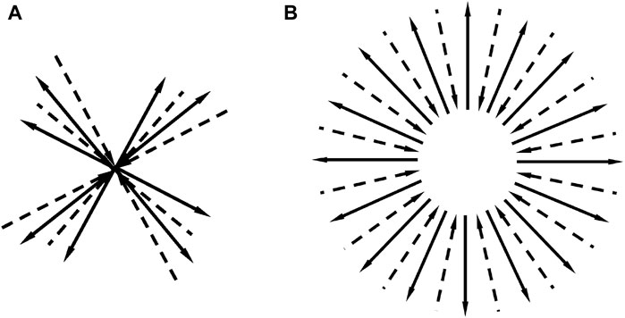
Figure 2. (A) Superposition of four Figure 1D in different directions. Incident and outgoing particles are represented by dashed and solid lines, respectively. (B) Superposition of a large number of similar collisions, which shows that in equilibrium, the momentum distribution is isotropic.

Reversing the directions of the arrows for both the solid and dashed lines shown in Figure 2B yields the schematic diagram of Eq. 61. This is a superposition of the schematic diagram shown in Figure 1C in all directions. This shows that for reciprocal collisions, as well as for reverse collisions, the momentum of the incoming and outgoing particles is uniformly distributed in all directions. This means that if there is a collision as shown in Figure 1A, then there will be a reverse collision (Figure 1C).

Therefore, although the detailed balance itself does not require the reverse process of a collision to appear, we believe that once the detailed balance is reached, then, in the equilibrium state, the reverse collision process of any collision also inevitably occurs. That a pair of reverse collisions, Figures 1A,C, occur in a macro-instant should be a by-product when an equilibrium state is reached.

We conceive a situation that slightly deviates from detailed balance.

When Boltzmann derived the H theorem, he obtained the following inequality [13]:

$\ln \frac{f\left({\mathit{p}}_1\right)f\left({\mathit{p}}_2\right)}{f\left({\mathit{p}}_1^{\prime }\right)f\left({\mathit{p}}_2^{\prime }\right)}\left[f\left({\mathit{p}}_1\right)f\left({\mathit{p}}_2\right)-f\left({\mathit{p}}_1^{\prime }\right)f\left({\mathit{p}}_2^{\prime }\right)\right]\ge 0.(62)$

The equal sign holds only when the detailed balance (Eq. 60) is reached. We suppose that the gas is very close to equilibrium, such that the momentum distribution of the two particles before the collision belongs to the equilibrium distribution with temperature T,

$f\left({\mathit{p}}_1\right)\propto \exp \left(-\frac{\epsilon \left({\mathit{p}}_1\right)}{k_{\mathrm{B}}T}\right),f\left({\mathit{p}}_2\right)\propto \exp \left(-\frac{\epsilon \left({\mathit{p}}_2\right)}{k_{\mathrm{B}}T}\right),(63)$

and after the collision, the distribution belongs to that with temperature $T+\Delta T$,

$f\left({\mathit{p}}_1^{\prime }\right)\propto \exp \left(-\frac{\epsilon \left({\mathit{p}}_1^{\prime }\right)}{k_{\mathrm{B}}\left(T+\Delta T\right)}\right),f\left({\mathit{p}}_2^{\prime }\right)\propto \exp \left(-\frac{\epsilon \left({\mathit{p}}_2^{\prime }\right)}{k_{\mathrm{B}}\left(T+\Delta T\right)}\right),(64)$

where

$\Delta T\ll T.(65)$

For an elastic collision (Eq. 59), the total energy before and after the collision is denoted by ε, $\epsilon =\epsilon \left({\mathit{p}}_1\right)+\epsilon \left({\mathit{p}}_2\right)=\epsilon \left({\mathit{p}}_1^{\prime }\right)+\epsilon \left({\mathit{p}}_2^{\prime }\right)$. We derive from Eq. 62 that

$-\frac{\epsilon }{k_{\mathrm{B}}}\left(\frac{1}{T}-\frac{1}{T+\Delta T}\right)\left(1-\exp \left[\frac{\epsilon }{k_{\mathrm{B}}}\left(\frac{1}{T}-\frac{1}{T+\Delta T}\right)\right]\right){\mathrm{e}}^{-\frac{\epsilon }{k_{\mathrm{B}}T}}\ge 0.(66)$

Regardless of whether the two molecules become a hotter or cooler distribution after the collision, this expression is not less than 0. It is equal to 0 only if $\Delta T=0$. Equations 63–66 mean that areas with slightly lower (higher) temperatures will increase (decrease) temperatures. Heat always flows from the hotter to the cooler area, making the temperature approach the same everywhere.

The isotropic distribution shown in Figure 2B is ideal only when the number of molecules in the gas approached infinity. In this equilibrium state, the momentum distribution remains unchanged.

Therefore, a necessary condition for achieving detailed balance is that the number of molecules in the gas is sufficiently large. Although the molecule number in the actual gas is as high as the order of magnitude of Avogadro constant, it is not really infinity after all. So, even in every macro-instant, it is not guaranteed that for every two-particle collision, there always occurs a corresponding reciprocal process. As a result, the momentum distribution of the molecule may deviate from the equilibrium distribution. This deviation is the fluctuation. Macrophysical quantities are averages calculated by means of the distribution function. Therefore, they fluctuate around their average values. Obviously, the larger the molecule number, the smaller the fluctuation.

Now, let us consider a region in the gas that is macroscopically small enough, say, a submillimeter-scale region, and the particle number in this region is much smaller than that of the whole gas. If in a region of 1 m³ there are $N\sim {10}^{23}$ particles, then, in ${10}^{-16}$ m³, there are $N_1\sim {10}^7$ particles, such that $N_1\ll N$. In such a small region, fluctuation will be comparatively large. It is possible that the number of particles with momentum in a certain direction in a macro-instant is much greater than that with opposite momentum. If a pollen granule is positioned in this region, the molecular impact it receives is not isotropic, so it suffers a net force. The pollen is subject to this force to move. This is the reason for Brownian motion, which reflects that in such a small area, detailed balance cannot be achieved.

Brownian motion also indicates that at a macro-instant, the number of particles entering and leaving the region is not always equal. That is to say, the density of particle numbers in this region varies with time. The molecular number density in different small regions at a micro-instant is not the same. The density varies around its average value. The fluctuation in a gas actually embodies the non-equilibrium at a micro-instant.

When the detailed balance is not achieved, the left and right sides of Eq. 60 are not equal. This means that at least a collision shown in Figure 1A does not have its reciprocal collision at a macro-instant. Consequently, the momentum distribution function will change. The gas cannot tend to be in equilibrium. Rather, it is in a non-equilibrium state. As a result, the macroscopic state may change.

Now, let us consider a case where an ideal gas expands into a vacuum, as shown in Figure 3. Figure 3A shows that the gas is confined in the left half of a box by a partition. At the initial moment, the partition is removed, and the gas begins to expand. The border line between the gas and vacuum is called frontline.

Figure 3

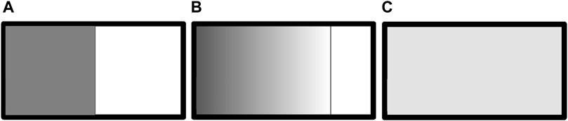
Figure 3. Schematic diagram of gas expansion into vacuum. The dotted line indicates the border line between gas and vacuum, called frontline. (A) The gas is confined inside the left half of the box by a partition. At the initial moment, the partition is drawn, and the gas starts expansion. (B) The gas expands to three-fourths of the box. (C) The gas is evenly distributed in the whole box, i.e., the equilibrium state is reached.

At the moment that the partition is just drawn, there is no particle on the right side of the frontline. We suppose that on the left side of the frontline, two particles moving rightward collide, as in Figure 1A, and after the collision, they enter the vacuum on the right side of the frontline. If a corresponding reciprocal collision of another two particles occurs, as in Figure 1D, they also enter the vacuum. At this moment, since there are no particles on the right side of the frontline, there is no reverse collision, as in Figure 1C. Therefore, the molecules always enter the vacuum from the left side of the frontline. There is no mechanism for particles to immediately return to the left side of the frontline. The frontline moves rightward.

Assuming that at the moment in Figure 3B, the momenta of all molecules in the gas are reversed, will the frontline move leftward? The analysis is actually the same as that for Figure 3A. Since the right side of the frontline is a vacuum, the molecules on the left side of the frontline still enter the vacuum, and there is no mechanism for particles to return to the left of the frontline. The frontline continues moving rightward. This shows that Loschmidt’s reasoning does not apply.

We next analyze the equilibrium state in Figure 3C. At every micro-instant, it is in a microstate. Every microstate in a macrostate is equiprobable to appear. For a microstate in the macrostate, when all the molecules’ momentum directions are reversed, the resultant is still a microstate in this macrostate. When a gas evolves from a non-equilibrium state to the equilibrium state as shown in Figure 3C, it can be any of these microstates. Conversely, any microstate in Figure 3C can be the one, denoted as A, that is achieved by reversing all the molecule momentum directions of a microstate, denoted as B, the latter being achieved from a non-equilibrium state. Following Loschmidt’s reasoning, we assume reversing all the molecular momentum in A to obtain state B, and with time, B will undergo a reverse process to go back to the original non-equilibrium state, such as in Figure 3B. However, we know that such a process has never occurred, and we do not expect so. This, again, shows that Loschmidt’s reasoning does not apply again.

On account of the molecule number in the gas considered not being infinite, when there is a collision (Figure 1A), the probability of its reverse collision (Figure 1C) is not 0. It seems that there is a nonzero probability for the reverse process of the gas to happen, say, from Figure 3C to Figure 3B. Nevertheless, this probability is so small that it is equivalent to impossibility. In Boltzmann’s language, the evolution from Figure 3B to Figure 3A or from Figure 3C to Figure 3B “has a definite calculable (though inconceivably small) probability, which approaches zero only in the limiting case when the number of molecules is infinite.” The time needed is so remote that “One may recognize that this is practically equivalent to never. …… If a much smaller probability than this is not practically equivalent to impossibility, then no one can be sure that today will be followed by a night and then a day” [57].

A frictionless quasi-static process is the exhibition of a series of equilibrium states. Therefore, such a process is reversible. However, this reversibility does not come from the reversibility of the motion of individual particles nor from the reversibility of the two-particle collision. Rather, it is the statistical average effect of a large number of molecules colliding with each other when the detailed balance is reached.

It is observed that macroscopic reversibility requires a large number of molecules in the gas. Usually, a gas contains molecules in the order of magnitude of the Avogadro constant, which is very close to meeting this requirement.

In summary, the motion of microscopic particles is irreversible. Nevertheless, when the number of molecules that make up the gas is very large, the macrostate of the gas can be in equilibrium when detailed balance is reached. The equilibrium state is the statistical average effect of the motion of a large number of microscopic molecules. Frictionless quasi-static processes are reversible.

3.3 Two-particle scattering in quantum mechanics

We showed in Subsection 2.5 that single-particle motion in QM is irreversible.

We [64] rigorously derived the generalized scattering formula in QM. The state of particles before (after) the scattering is called the initial (final) state. For single-particle scattering, if the initial state is a plane wave of a free particle, ${\mathrm{e}}^{\mathrm{i}\mathit{p}\cdot \mathit{r}}$, after being scattered by a scattering center, the final state is a complicated spherical wave function $\psi \left(\mathit{r},t\right)$. This spherical wave has projected amplitudes on plane waves ${\mathrm{e}}^{\mathrm{i}{\mathit{p}}^{\prime }\cdot \mathit{r}}$ in all directions.

Let us discuss two-particle scattering. Suppose that two free particles with momenta ${\mathit{p}}_1$ and ${\mathit{p}}_2$ collide. The initial state is the product of two plane waves, ${\mathrm{e}}^{\mathrm{i}{\mathit{p}}_1\cdot {\mathit{r}}_1}{\mathrm{e}}^{\mathrm{i}{\mathit{p}}_2\cdot {\mathit{r}}_2}$. The final state $\psi \left({\mathit{r}}_1,{\mathit{r}}_2;t\right)$ is complex, which can spread in all directions. If we intend to implement the reverse process of the scattering, we must prepare $\psi \left({\mathit{r}}_1,{\mathit{r}}_2;t\right)$ as the initial state for the reverse process, which is apparently impossible. So, this scattering process of two free particles in QM is irreversible.

Nevertheless, $\psi \left({\mathit{r}}_1,{\mathit{r}}_2;t\right)$ can be expanded by two-particle plane waves, i.e., it has project amplitude on every pair of plane waves ${\mathrm{e}}^{\mathrm{i}{{\mathit{p}}^{\prime }}_1\cdot {\mathit{r}}_1}{\mathrm{e}}^{\mathrm{i}{{\mathit{p}}^{\prime }}_2\cdot {\mathit{r}}_2}$. That is to say, there is a probability for the two particles with momenta ${\mathit{p}}_1$ and ${\mathit{p}}_2$ to transit to two plane waves with specific momenta ${\mathit{p}}_1^{\prime }$ and ${\mathit{p}}_2^{\prime }$, respectively. This probability is denoted as $w\left({\mathit{p}}_1,{\mathit{p}}_2;{\mathit{p}}_1^{\prime },{\mathit{p}}_2^{\prime }\right)$. In Figure 1, we use a piece of arrowed line to represent a plane wave with momentum. Figure 1A shows a sketch of the two $\left({\mathit{p}}_1,{\mathit{p}}_2\right)$ plane waves transiting to two new plane waves $\left({\mathit{p}}_1^{\prime },{\mathit{p}}_2^{\prime }\right)$, denoted as $\left({\mathit{p}}_1,{\mathit{p}}_2\right)\to \left({\mathit{p}}_1^{\prime },{\mathit{p}}_2^{\prime }\right)$. Figures 1B,C,D show the time-inverse transition, reverse transition, and reciprocal transitions, respectively, of Figure 1A. All of the transitions follow the total energy conservation and total momentum conservation (Eq. 59). The transition probability of the reciprocal process is denoted as $w\left({\mathit{p}}_1^{\prime },{\mathit{p}}_2^{\prime };{\mathit{p}}_1,{\mathit{p}}_2\right)$.

We have rigorously proved that [64]

$w\left({\mathit{p}}_1,{\mathit{p}}_2;{\mathit{p}}_1^{\prime },{\mathit{p}}_2^{\prime }\right)=w\left({\mathit{p}}_1^{\prime },{\mathit{p}}_2^{\prime };{\mathit{p}}_1,{\mathit{p}}_2\right).(67)$

The transition probability of the process (Figure 1A) $\left({\mathit{p}}_1,{\mathit{p}}_2\right)\to \left({\mathit{p}}_1^{\prime },{\mathit{p}}_2^{\prime }\right)$ is the same as that of (Figure 1D) $\left({\mathit{p}}_1^{\prime },{\mathit{p}}_2^{\prime }\right)\to \left({\mathit{p}}_1,{\mathit{p}}_2\right)$. This conclusion is derived from the scattering theory in QM, so it is always valid, irrespective of whether a system reaches detailed balance, as well as irrelevant to the properties of the whole gas [74].

The previous discussion about the two-particle collisions and detailed balance in classical mechanics is entirely applicable to the case here, as long as the two-particle collision in classical mechanics is replaced by the scattering transition of two free particles, $\left({\mathit{p}}_1,{\mathit{p}}_2\right)\to \left({\mathit{p}}_1^{\prime },{\mathit{p}}_2^{\prime }\right)$, in QM. In particular, the detailed balance only concerns a pair of reciprocal scattering transitions (Figures 1A,D) and is irrelative to the reverse transition (Figure 1C).

If a scattering transition (Figure 1A) occurs, the probability of the occurrence of its reverse process (Figure 1C) is equal to 1, and the original process (Figure 1A) is said reversible. However, it is actually that $w\left({\mathit{p}}_1,{\mathit{p}}_2;{\mathit{p}}_1^{\prime },{\mathit{p}}_2^{\prime }\right)<1$. Similarly, the probability that the process (Figure 1C) occurs is necessarily less than 1. Therefore, the process (Figure 1A) is irreversible.

It was believed that [50, 51]

$w\left({\mathit{p}}_1,{\mathit{p}}_2;{\mathit{p}}_1^{\prime },{\mathit{p}}_2^{\prime }\right)=w\left(-{\mathit{p}}_1^{\prime },-{\mathit{p}}_2^{\prime };-{\mathit{p}}_1,-{\mathit{p}}_2\right).(68)$

This relationship means that the transition probabilities of the processes in Figures 1A,B are the same. This was called detailed balance and seemed to be obtained from QM [75], the authors of which equated the time-inverse and reverse processes. We stress that in deriving scattering formulas [64], we always considered clockwise processes. We do not know how to include the clockwise and anticlockwise processes in one formula. In Section 2, it is observed that the retarded and advanced processes have to be studied separately. Therefore, we can prove Eq. 67 but are unable to verify Eq. 68 by the scattering theory in QM.

We address three points here. First, we make it clear that detailed balance (Eq. 60), but not (Eq. 67), is a content in statistical mechanics. Eq. 67 is proved by the scattering theory in QM. Second, Eq. 60 is expressed by momentum distribution function, which involves all molecules in the gas, while Eq. 67 only concerns two molecules, irrelevant of other molecules. Third, Eq. 60 only applies to equilibrium states, while Eq. 67 is always correct for two-particle scattering, regardless of whether the whole gas reaches equilibrium.

In [50], Eq. 68 is put down first. Then, with known Maxwell–Boltzmann distribution for equilibrium state, it is postulated that the numbers of the collision and reverse collision in unit time and unit phase space volume are the same so as to achieve Eq. 60. This procedure is different from that used by Boltzmann, who first obtained Eq. 60 for equilibrium state and then derived Maxwell–Boltzmann distribution from Eq. 60.

We next discuss the collision between two non-free particles. That is to say, before and after the collision, particles may be in bound states. A non-free particle is also called a bound particle. On account of the identity of particles, detailed balance should be written in the following form [11, 13, 15, 73]:

$\begin{array}{l}{n}_i{n}_j\left(1+\chi n_{i^{\prime }}\right)\left(1+\chi n_{j^{\prime }}\right)=n_{i^{\prime }}{n}_{j^{\prime }}\left(1+\chi n_i\right)\left(1+\chi n_j\right),\\ \left\{\begin{array}{l}\chi =0,\text{Distinguishable particles}\\ \chi =+1,\text{Bosons}\\ \chi =-1,\text{Fermions}\end{array}\right.\end{array}.(69)$

In Eq. 69, $n_i$ is the average number of particles in the energy state ${\epsilon }_i$. From the left- to right-hand sides, Eq. 69 shows that two particles in the energy levels ${\epsilon }_i$ and ${\epsilon }_j$ collide and then transit to energy levels ${\epsilon }_{i^{\prime }}$ and ${\epsilon }_{j^{\prime }}$, respectively, denoted as $\left(i,j\to i^{\prime },j^{\prime }\right)$. From the right- to left-hand sides, Eq. 69 refers to its reciprocal process, $\left(i^{\prime },j^{\prime }\to i,j\right)$. The transition probabilities of the two processes are denoted by $w\left(i,j\to i^{\prime },j^{\prime }\right)$ and $w\left(i^{\prime },j^{\prime }\to i,j\right)$, respectively. Just as in Eq. 67, it should be

$w\left(i,j\to i^{\prime },j^{\prime }\right)=w\left(i^{\prime },j^{\prime }\to i,j\right).(70)$

In the reciprocal courses, the total energy is conserved.

${\epsilon }_i+{\epsilon }_j={\epsilon }_{i^{\prime }}+{\epsilon }_{j^{\prime }}.(71)$

Note the difference in the collision of the two bound particles and two free particles. A free particle has momentum. Its state has an index momentum. In its reverse motion, its momentum direction is opposite to that in its original motion. This direction reversion helps us distinguish the reverse and reciprocal motions, e.g., Figures 1C,D. In both original and reverse motions, its total energy and total momentum are conserved (see Eq. 59a, b).

A bound particle is in one of its discrete energy levels, and there is no momentum in such a state index. Thus, a collision requires the conservation of total energy (see Eq. 71) without the relationship of momentum conservation. In this case, there is no difference between reverse and reciprocal collisions.

Some scholars believed that the collisions are reversible. The reason may be the identity of the reverse and reciprocal collisions of bound particles. We reiterate the definition of the reversibility of a process: if after an original process $\left(i,j\to i^{\prime },j^{\prime }\right)$ occurs, the occurrence probability of the reverse process $\left(i^{\prime },j^{\prime }\to i,j\right)$ is less than 1, i.e., $w\left(i^{\prime },j^{\prime }\to i,j\right)<1$, then the original process is irreversible. This is because the particles in the state $\left(i,j\right)$ can also transit to states other than states $\left(i^{\prime },j^{\prime }\right)$ by collision, as long as Eq. 71 is met. The conclusion is that in any case, two-particle collisions are irreversible.

[76] thought that Eq. 67 was a microreversibility relation. [77] thought that Eq. 67 meant the detailed balance: “This notion is based solely on the reversibility of the microscopic equation of motion. (Or, more technically, on the Hermitian nature of the scattering Hamiltonian).” The detailed balance Eq. 69 only involves the distribution function and has nothing to do with whether the equation of motion is reversible. Moreover, the two-particle scattering transition is irreversible. We emphasize that when deriving Eq. 67, we do not use the time inversion invariance of the microscopic equations of motion [64].

For the cases of two free particle collisions, that equilibrium is reached is not due to the reversibility of the collision, but from detailed balance (Eq. 60). Similarly, in the case of bound particle collisions, equilibrium is not due to the reversibility of the collisions, but due to Eq. 69. In the case of quantum statistics, detailed balance can be obtained by master equations, although in a form superficially different from Eq. 69 [9, 11, 52]. Using the form of master equations, it is possible to define a “distance” measuring the violation of detailed balance [19].

4 Conclusion

In this work, by careful analysis, we find that the motions of microscopic particles are irreversible.

We first distinguish between the concepts of equation of motion and specific motion. These two concepts have different mathematical expressions. An equation of motion is just a differential equation that embodies the laws of motion, which can be of invariance under time inversion, but it does not describe any specific motion. A specific motion is a specific solution solved from the equation of motion after considering the initial conditions. It represents the relationship between physical quantities over time and can be graphically illustrated.

We then distinguish between the concepts of time-inverse motion and reverse motion. The former is counterclockwise, which is a fictional movement, and the latter is clockwise. In both classical mechanics and quantum mechanics, we provide mathematical expressions for time-inverse motion and reverse motion. The former is described by a time-advanced function and the latter by a time-retarded function. From the mathematical derivation, we conclude that the single-particle motion process is irreversible.

A system consisting of a large number of molecules frequently colliding with each other is called a collision system. In such a system, the microscopic mechanism that plays a decisive role is two-particle collision.

A careful analysis of the two-particle collision was carried out. Three cases are considered: two-particle collision in classical mechanics, the collisions of two free particles, and two bound particles in quantum mechanics. For the cases of two free particle collisions, a distinction is made between reverse collision and reciprocal collision. This difference stems from the fact that there is a momentum index of the state of the particle. For the two bound particle collisions, there is no difference between these two collisions because there is no momentum index in the state of a particle.

We have defined the reversibility for the three cases of two-particle collisions. By definition, all these collision processes are irreversible.

The irreversibility of the microscopic two-particle collisions determines that, generally speaking, the macroscopic processes of gases are irreversible.

However, the occurrence of a large number of collisions can make a gas reach detailed balance. The detailed balance means that the combination of a two-particle collision and its reciprocal collision retains the distribution function of the gas unchanged. This is the equilibrium state. The detailed balancing does not have the meaning of micro-reversibility. The prerequisite for achieving the detailed balance is that the number of molecules in the gas is sufficiently large.

In summary, every specific microprocess is essentially irreversible. The statistical nature of a large number of microprocesses can lead to the reversibility of certain macroprocesses. Thereby, we explain the microscopic mechanism of why the processes of gases can be irreversible.

Data availability statement

The original contributions presented in the study are included in the article/Supplementary Material; further inquiries can be directed to the corresponding author.

Author contributions

H-YW: conceptualization, data curation, formal analysis, funding acquisition, investigation, methodology, project administration, resources, software, supervision, validation, visualization, writing–original draft, and writing–review and editing.

Funding

The author(s) declare that financial support was received for the research, authorship, and/or publication of this article. This work was supported by the National Natural Science Foundation of China under Grant No. 12234013 and the National Key Research and Development Program of China under Nos. 2018YFB0704304 and 2016YFB0700102.

Conflict of interest

The author declares that the research was conducted in the absence of any commercial or financial relationships that could be construed as a potential conflict of interest.

Publisher’s note

All claims expressed in this article are solely those of the authors and do not necessarily represent those of their affiliated organizations, or those of the publisher, the editors, and the reviewers. Any product that may be evaluated in this article, or claim that may be made by its manufacturer, is not guaranteed or endorsed by the publisher.

References

1. Swendsen RH. Irreversibility and the thermodynamic limit. J Stat Phys (1974) 10(2):175–7. doi:10.1007/BF01009719

CrossRef Full Text | Google Scholar

2. Swendsen RH. Explaining irreversibility. Am J Phys (2008) 76(7):643–8. doi:10.1119/1.2894523

CrossRef Full Text | Google Scholar

3. Lebowitz JL. Boltzmann’s entropy and time’s arrow. Phys Today (1993) 46(9):32–8. doi:10.1063/1.881363

CrossRef Full Text | Google Scholar

4. Lebowitz JL. Macroscopic laws, microscopic dynamics, time’s arrow and Boltzmann’s entropy. Physica A (1993) 194:1–27. doi:10.1016/0378-4371(93)90336-3

CrossRef Full Text | Google Scholar

5. Lebowitz JL. Statistical mechanics: a selective review of two central issues. Rev Mod Phys (1999) 71(2):S346–57. doi:10.1103/RevModPhys.71.S346

CrossRef Full Text | Google Scholar

6. Lebowitz JL. Microscopic origins of irreversible macroscopic behavior. Physica A (1999) 263:516–27. doi:10.1016/S0378-4371(98)00514-7

CrossRef Full Text | Google Scholar

7. Liboff RL. Introduction to the theory of kinetic equations. New York: John Wiley & Sons, Inc. (1969).

Google Scholar

8. Evans DJ, Searles DJ. The fluctuation theorem. Adv Phys (2002) 51(7):1529–85. doi:10.1080/00018730210155133

CrossRef Full Text | Google Scholar

9. Bellac ML, Mortessagne F, Batroun GG. Equilibrium and non-equilibirum statistical thermodynamics. Cambridge: Cambridge University Press (2004).

Google Scholar

10. Schwable F. Statistical mechanics. 2nd ed. Berlin, Heidelberg: Springer-Verlag (2006). Chapter 10.

Google Scholar

11. Vliet CMV. Equilibrium and non-equilibrium statistical mechanics. Singapore, Hackensack, NJ: World Scientific Pub (2008).

Google Scholar

12. Krapivsky PL, Redner S, Ben-Naim E. A kinetic view of statistical physics. Cambridge, New York: Cambridge University Press (2010).

Google Scholar

13. Tolman RC. The principles of statistical mechanics. New York: Dover Publications (1979).

Google Scholar

14. Landau LD, Lifshitz EM. Statistical physics Part 1 vol. 5 of course of theoretical physics. New York: Pergmon Press (1980). Chapter 1.

Google Scholar

15. Haar Dter. Foundations of statistical mechanics. Rev Mod Phys (1955) 27(3):289–338. doi:10.1103/RevModPhys.27.289

CrossRef Full Text | Google Scholar

16. Evans DJ, Searles DJ, Williams SR. Fundamentals of classical statistical thermodynamics dissipation, relaxation and fluctuation theorem. Weinheim, Germany: Wiley-VCH Verlag GmbH & Co. KGaA, Boschstr (2016), 69469.

Google Scholar

17. Tanimura Y. Numerically “exact” approach to open quantum dynamics: the hierarchical equations of motion (HEOM). J Chem Phys (2020) 153:020901. doi:10.1063/5.0011599

PubMed Abstract | CrossRef Full Text | Google Scholar

18. Barbier M, Gaspard P. Microreversibility and the statistics of currents in quantum transport. Phys Rev E (2020) 102:022141. doi:10.1103/PhysRevE.102.022141

PubMed Abstract | CrossRef Full Text | Google Scholar

19. Platini T. Measure of the violation of the detailed balance criterion: a possible definition of a “distance” from equilibrium. Phys Rev E (2011) 83:011119. doi:10.1103/PhysRevE.83.011119

PubMed Abstract | CrossRef Full Text | Google Scholar

20. Prigogine I. Non-equilibrium statistical mechanics. Mineola, New York: Dover Publications, Inc. (2017). p. 255.

Google Scholar

21. Evans DJ, Cohen EGD, Morris GP. Probability of 2nd Law violations in shearing steady-states. Phys Rev Lett (1993) 71:2401–4. doi:10.1103/PhysRevLett.71.2401

PubMed Abstract | CrossRef Full Text | Google Scholar

22. Evans DJ, Searles DJ. Equilibrium microstates which generate second Law violating steady states. Phys Rev E (1994) 50:1645–8. doi:10.1103/PhysRevE.50.1645

PubMed Abstract | CrossRef Full Text | Google Scholar

23. Dorosz S, Pleimling M. Fluctuation ratios in the absence of microscopic time reversibility. Phys Rev E (2009) 79:030102. doi:10.1103/PhysRevE.79.030102

PubMed Abstract | CrossRef Full Text | Google Scholar

24. Peres A. Quantum theory: concepts and methods. New York: Kluwer Academics Publishers (2002). p. 347.

Google Scholar

25. Langmuir I. J Am Chem Soc (1916) 38:2221–95. doi:10.1021/ja02268a002

CrossRef Full Text

26. Frisch HL. Poincare recurrences. Phys Rev (1956) 104(1):1–5. doi:10.1103/PhysRev.104.1

CrossRef Full Text | Google Scholar

27. Liboff RL. Kinetic theory, classical, quantum, and relativistic descriptions. 3rd ed. Berlin: Spinger-Verlag New York, Inc (2003).

Google Scholar

28. Hahn EL. Spin echoes. Phys Rev (1950) 80(4):580–94. doi:10.1103/PhysRev.80.580

CrossRef Full Text | Google Scholar

29. Hahn EL. Free nuclear induction. Phys Today (1953) 6(11):4–9. doi:10.1063/1.3061075

CrossRef Full Text | Google Scholar

30. Rothstein J. Nuclear spin echo experiments and the foundations of statistical mechanics. Am J Phys (1957) 25:510–8. doi:10.1119/1.1934539

CrossRef Full Text | Google Scholar

31. Reif R. Statistical physics berkeley physics course. McGraw-Hill, Inc. (1965). p. 50.

Google Scholar

32. Orban J, Bellemans A. Velocity-inversion and irreversibility in a dilute gas of hard disks. Phys Lett A (1967) 24(11):620–1. doi:10.1016/0375-9601(67)90651-2

CrossRef Full Text | Google Scholar

33. Brilliantov NV, Poschel T. Kinetic theory of granular gases. Oxford: Oxford University Press (2004). p. 128.

Google Scholar

34. Fermi E, Pasta J, Ulam E, Tsinghou M. Studies of nonlinear systems. Report LA-1940. Los Alamos Scientific Laboratory of the University of California (1955). Available from: https://people.math.umass.edu/∼kevrekid/math697wa/ACC0041.pdf (Accessed September 25, 2023).

Google Scholar

35. Zabusky NJ, Kruskal MD. Interaction of “solitons” in a collision less plasma and the recurrence of initial states. Phys Rev Lett (1965) 15(6):240–3. doi:10.1103/PhysRevLett.15.240

CrossRef Full Text | Google Scholar

36. Tuck JL, Menzel MT. The superperiod of the nonlinear weighted string (FPU) problem. Adv Math (1972) 9(3):399–407. doi:10.1016/0001-8708(72)90024-2

CrossRef Full Text | Google Scholar

37. Walker GH, Ford J. Amplitude instability and ergodic behavior for conservative nonlinear oscillator systems. Phys Rev (1969) 188(1):416–32. doi:10.1103/PhysRev.188.416

CrossRef Full Text | Google Scholar

38. Lunsford GH, Ford J. On the stability of periodic orbits for nonlinear oscillator systems in regions exhibiting stochastic behavior. J Mat Phys (1972) 13(5):700–5. doi:10.1063/1.1666037

CrossRef Full Text | Google Scholar

39. Lebowitz JL, Penrose O. Modern ergodic theory. Phys Today (1973) 23(2):23–9. doi:10.1063/1.3127948

CrossRef Full Text | Google Scholar

40. Hasegawa H. Responses to applied forces and the Jarzynski equality in classical oscillator systems coupled to finite baths: an exactly solvable nondissipative nonergodic model. Phys Rev E (2011) 84:011145. doi:10.1103/PhysRevE.84.011145

PubMed Abstract | CrossRef Full Text | Google Scholar

41. Li J, He D. Finite-time fluctuation theorem for oscillatory lattices driven by a temperature gradient. Phys Rev E (2021) 103:062122. doi:10.1103/PhysRevE.103.062122

PubMed Abstract | CrossRef Full Text | Google Scholar

42. Palmer RD. Broken ergodicity. Adv Phys (1982) 31(6):669–735. doi:10.1080/00018738200101438

CrossRef Full Text | Google Scholar

43. JackGarrahan RLJP. Metastable states and space-time phase transitions in a spin-glass model. Phys Rev E (2010) 81:011111. doi:10.1103/PhysRevE.81.011111

PubMed Abstract | CrossRef Full Text | Google Scholar

44. Frisch HL. An approach to equilibrium. Phys Rev (1958) 109(1):22–9. doi:10.1103/PhysRev.109.22

CrossRef Full Text | Google Scholar

45. Wang H-Y. Liouville equation in statistical mechanics is not applicable to gases composed of colliding molecules. Phys Essays (2023) 36(1):13–21. doi:10.4006/0836-1398-36.1.13

CrossRef Full Text | Google Scholar

46. Born M, Green HS. A general kinetic theory of liquids; the molecular distribution functions. Proc R Soc Lond Ser A Math Phys Sci (1946) 188(1012):10–8. doi:10.1098/rspa.1946.0093

PubMed Abstract | CrossRef Full Text | Google Scholar

47. Kirkwood JG. The statistical mechanical theory of transport processes I. General theory. J Chem Phys (1946) 14(3):180–201. doi:10.1063/1.1724117

CrossRef Full Text | Google Scholar

48. Kirkwood JG. The statistical mechanical theory of transport processes II. Transport in gases. J Chem Phys (1947) 15(1):72–6. doi:10.1063/1.1746292

CrossRef Full Text | Google Scholar

49. Boer J. Molecular distribution and equation of state of gases. Rep Prog Phys (1949) 12:305–74. doi:10.1088/0034-4885/12/1/314

CrossRef Full Text | Google Scholar

50. Lifshitz EM, Pitaevskii LP. Physical kinetics, vol. 10 of course of theoretical physics. Oxford: Pergamon Press (1981). Chapter 1.

Google Scholar

51. Huang K. Statistical mechanics. 2nd ed. New York: John Wiley & Sons (1987).

Google Scholar

52. Reichl LE. A modern course in statistical physics. 2nd ed. New York: John Welei & Sons, Inc. (1998).

Google Scholar

53. Tessarotto M, Cremaschini C. First-principle proof of the modified collision boundary conditions for the hard-sphere system. Phys Lett A (2014) 378:1760–6. doi:10.1016/j.physleta.2014.04.054

CrossRef Full Text | Google Scholar

54. Tessarotto M, Cremaschini C. Modified BBGKY hierarchy for the hard-sphere system. Eur Phys J Plus (2014) 129:243. doi:10.1140/epjp/i2014-14243-7

CrossRef Full Text | Google Scholar

55. Abramov R. The random gas of hard spheres. J (Multidisciplinary Scientific Journal) (2019) 2:162–205. doi:10.3390/j2020014

CrossRef Full Text | Google Scholar

56. Abramov R. Correction: abramov, R. The random gas of hard spheres. J (Multidisciplinary Scientific Journal) (2020) 3:324–8. doi:10.3390/j3030025

CrossRef Full Text | Google Scholar

57. Boltzmann L. Lectures on gas theory. In: Courier corporation. New York: Dover Publications, Inc. (2012).

Google Scholar

58. Evans DJ, Searles DJ. Causality, response theory, and the second law of thermodynamics. Phys Rev E (1996) 53(6):5808–15. doi:10.1103/PhysRevE.53.5808

PubMed Abstract | CrossRef Full Text | Google Scholar

59. Bjorken JD, Drell SS. Relativistic quantum mechanics. New York: McGraw-Hill Book Co. (1964).

Google Scholar

60. Kleinert H. Path integrals in quantum mechanics, statistics, polymer physics, and financial markets. 5th ed. Singapore: World Scientific Publishing Co. Pte. Ltd. (2009). Chap. 1.

Google Scholar

61. Greiner W, Reinhardt J. Quantum electrodynamics. 4th ed. Berlin, Heidelberg: Springer-Verlag (2009).

Google Scholar

62. Wachter A. Relativistic quantum mechanics. Dordrecht: Springer Science + Business Media B. V (2010). p. 978–3644. doi:10.1007/978-90-481-3645-2

CrossRef Full Text | Google Scholar

63. Wang H-Y. The mathematical physical equations that the retarded and advanced Green’s functions satisfy. Phys Essays (2022) 35(4):380–91. doi:10.4006/0836-1398-35.4.0

CrossRef Full Text | Google Scholar

64. Wang H-Y. A generalized scattering theory in quantum mechanics. J Phys Commun (2023) 7:075001. doi:10.1088/2399-6528/acde44

CrossRef Full Text | Google Scholar

65. Wang H-Y. Green’s function in condensed matter physics. Beijing: Alpha Science International ltd. and Science Press (2012).

Google Scholar

66. Wang H-Y. Mathematics for physicists. Singapore and Beijing: World Scientific Publishing Company and Science Press (2017).

Google Scholar

67. Sakurai JJ. Modern quantum mechanics. Addison-Wesley Publishing Company, Inc. (1994).

Google Scholar

68. Kestin J, Dorfman JR. A course in statistical thermodynamics. New York: Academic Press, Inc. (1971).

Google Scholar

69. Chapman S, Cowling TG. The mathematical theory of non-uniform gases an account of the kinetic theory of viscosity. In: Thermal conduction and diffusion in gases. 3rd ed. Cambridge: Cambridge University Press (1970).

Google Scholar

70. Tien CL, Lienhard JH. Statistical thermodynamics. Washington, New York: Hemisphere Pub. Corp. (1979).

Google Scholar

71. Isihara A. Statistical physics. New York: Academic Press, Inc. (1971).

Google Scholar

72. Landau LD, Lifshitz EM. Mechanics vol. 1 of course of theoretical physics. 3rd ed. New York: Pergmon Press (1976).

Google Scholar

73. Toda M, Kubo R, Saito N. Statistical physics I equilibrium statistical mechanics. Berlin, Hedelberg: Springer-Verlag (1983).

Google Scholar

74. Hakim R. Introduction to relativistic statistical mechanics classical and quantum. Singapore: World Scientific Publishing Co. Pte. Ltd. (2011).

Google Scholar

75. Landau LD, Lifshitz EM. Quantum mechanics non-relativistic theory vol. 3 of course of theoretical physics. 3rd ed. New York: Pergmon Press (1977). Chap. 18.

Google Scholar

76. Messiah A. Quantum mechanics II. 2nd ed. Mineloa, New York: John Wiley & Sons, Inc. (1962). Chap. 19.

Google Scholar

77. Mattis DC, Swendsen RH. Statistical mechanics made simple. 2dn ed. Singapore: World Scientific (2008).

Google Scholar