Decomposing the percolation backbone reveals novel scaling laws of the current distribution

The distribution of currents on critical percolation clusters is the fundamental quantity describing the transport properties of weakly connected systems. Nevertheless, its finite-size extrapolation is still one of the outstanding open questions concerning disordered media. By hierarchically decomposing the 3-connected components of the backbone, we disclose that the current distribution is determined from two distributions, namely, the one corresponding to the number of bonds in each level and another one corresponding to the factors by which the current is reduced, when going from one level to the next. The first distribution follows a finite-size scaling, while the second is a power law with an exponent consistent with 3/4 in two dimensions. The standard hierarchical model for the backbone is too simple to reproduce this complex scenario. Our new decomposition method of the backbone also allows to calculate much smaller currents than before, attaining a precision of 10⁻³⁵ and systems of size L = 8192². Moreover, our method is not restricted to electric currents on critical percolation clusters but could also be applied to other transport problems on sparse graphs including fluid flow and car traffic.

1 Introduction

Percolation was originally proposed to model the flow through a porous medium [1] but has since turned out to be a fundamental model in statistical physics [2], serving as a geometrical template for phase transitions with multiple applications in physics and beyond, including the sol–gel transition, the onset of fluid flow, the conductivity of random media, opinion dynamics, and the outbreak of epidemics. An important issue in percolation theory is the solution of linear transport at criticality [3]. Under such a framework, one replaces the bonds of a percolation cluster by Ohmic resistors and applies a potential difference between two distant sites on this cluster. Solving the set of linear equations given by Kirchhoff’s nodal rule at each node yields the currents at each bond. This linear transport problem in percolation has many applications. Examples include flow through porous materials [4–8], oil production [9], and conductivity of semiconducting materials or metal–insulator mixtures [10].

The distribution of the currents on the percolation cluster at criticality has been found to be multifractal [11] since different moments exhibit unrelated scaling exponents. However, its multifractal spectrum f(α) strongly depends on the system size [12]. Despite the great controversy generated about the asymptotic behavior of the distribution for weak currents and large systems [13–15], no satisfactory solution has been found yet [12].

By definition, a 3-connected component (3CC) is the set of nodes of a graph that remains connected after any two bonds are removed [16]. It should be noted that simple parallel and series conformations cannot form 3CCs. This concept can be directly associated with physical partitioning and has been very useful in the solution of several problems in graph theory [16, 17]. For instance, the partition of the critical conducting backbone in 3CCs has been successfully used to demonstrate that these components are also fractal [18], like other structures in critical percolation [19].

Here, we will focus precisely on weak currents and large system sizes to introduce a new way to calculate the current distribution in the critical conducting backbone based on its hierarchical partition in terms of 3-connected components. The backbone is the part of the infinite cluster that takes part in the conduction. Formally, the backbone is defined as the union of the sets of self-avoiding paths that connect two extremes of the cluster. By taking advantage of the partition of the backbone on 3CCs, we are able to solve subsets of coupled linear equations in sequence, starting from 3CCs on the smallest scale. As illustrated in Figure 1, the solution of the electrical transport problem on these components allows determining their effective resistances. By replacing these 3CCs to their corresponding effective conductances, the Kirchhoff problem can then be sequentially solved on larger and larger 3CC scales, up to the scale of the critical backbone itself.

FIGURE 1

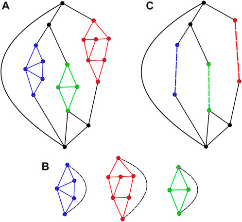
FIGURE 1. Formally, a 3-connected component (3CC) is the set of nodes in a graph that will remain in the same component after any two bonds are removed [16]. For a physicist, however, an intuitive definition may be any subset of the graph that connects to the rest only at a pair of articulating nodes and is not formed by simple parallel and/or series conformations. The hierarchical partition of a graph in 3CCs can be used to solve efficiently the Kirchhoff problem [16]. In panel (A), we show a graph with four 3CCs. After solving the Kirchhoff problem for the three 3CCs shown in (B), these components can be replaced by effective resistances, simplifying the solution of 3CC on a larger scale, as shown in (C).

1.1 Hierarchical structure of the conducting backbone

It has been proposed that the conducting backbone can be separated in blobs and red bonds, with the red bonds being the connections that are removed to split the backbone into two separate parts, while the blobs are the parts of the conducting backbone that are multi-connected, that is, that remain connected after the removal of any bond. Here, we expand on this idea using the concept of 3CCs. In our definition, 3CCs at the largest scale, namely, the blobs of the backbone, are of level 1, and components of level 2 are those that are replaced by effective bonds in components of level 1, and so on, with components of one level replacing effective bonds in the components of the level below. It should be reminded that sets of bonds in simple parallel and series conformations, despite being connected to the rest of the graph at just two points, do not form 3CCs. Therefore, one needs to include factors of level 0, accounting for splits of the current that take place outside all 3CCs. A typical example of the critical conducting backbone is shown in Figure 2, where the bonds are colored according to their 3CC levels, clearly indicating the underlying hierarchical structure of the partition.

FIGURE 2

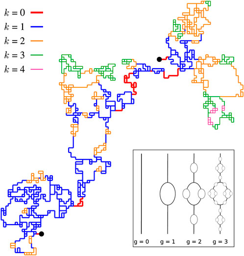
FIGURE 2. Typical critical backbone with bonds colored by level. Bonds of level k are those inside a 3CC of level k but outside 3CCs of level k + 1. The black dots indicate the pole nodes, between which a potential difference is applied. The inset shows the hierarchical model proposed in [11]. Inspired by the self-similarity property of the conducting backbone, this simple model can be solved analytically to compute the current distribution. Higher generations g reveal smaller scales. Considering that every bond has the same resistance, the current passing through resistor ℓ will be given by $I_{\ell }=I_t{2}^{-n_{\ell }}$, where I_t is the total current, and the numbers n_ℓ follow a binomial distribution, resulting in a log-normal distribution for the currents [20]. However, although the critical backbone in the main figure is self-similar and presents a hierarchical structure [18], the current distribution does not follow a log-normal relation [12].

The idea that the structure of critical percolation clusters can be described in terms of a hierarchical model to determine the current distribution has been originally suggested in [20]. In this model, as shown in the inset of Figure 2, each bond ℓ has a current $I_{\ell }=I_t{2}^{-n_{\ell }}$, where I_t is the total current through the lattice, and the exponents n_ℓ are distributed according to a binomial distribution. As a result, the currents follow a log-normal distribution and exhibit multifractal properties [20]. Unfortunately, the clever approach proposed in [20] does not succeed in describing the current distribution on critical conducting backbones since their distribution is not log-normal [12]. This deviation from a log-normal may seem surprising since the critical conducting backbone is self-similar and presents a hierarchical structure [18]. Even more surprising is the fact that the current distribution on the critical backbone does not appear to follow consistent finite-size scaling laws since the distribution assumes different shapes at different scales [12].

2 Methods

Taking advantage of the partition in 3-connected components, the complex problem of a large conducting backbone, with a large number of unknown variables, is replaced by a series of steps. At each step, a single Kirchhoff problem is solved for a single 3CC, which will be replaced by an effective bond when solving the component at a larger scale. In this way, at each step, the number of variables is much smaller. Since the complexity of solving these sets of coupled equations grows super-linearly, for large system sizes, the time gained by reducing the rank of the equations should, therefore, compensate the pre-processing step to obtain the partition. To give an idea of the advantage of employing this decomposition, in two dimensions, the number of nodes in the backbone scales with the system size L as M_b ∼ L^1.64 [21], while the largest 3CC scales as M₃ ∼ L^1.15 [18].

After using the partition in 3-connected components to solve the Kirchhoff problem on the conducting backbone, we proceed with the recovering of the current distribution. To obtain the current through a given bond ℓ, we need to collect the information from every component containing this bond. Each bond will carry a fraction $f_{\ell }={\prod }_{j=0}^k{f}_{j\ell }$ of the total current, where the factors f_jℓ must be determined by solving the Kirchhoff problem on the 3CC at level j, as shown in Figure 3. The number of factors in this product is equal to the level k of the bond, that is, the number of 3CCs where bond ℓ is nested. At each step of the hierarchical solution, the current in each effective bond is typically a significant portion of the current passing through the component. However, when the factors of several nested components are multiplied to obtain the final current of a given bond, the result can be many orders of magnitude smaller than the total current. As a consequence, our hierarchical approach allows in accurately obtaining a current distribution that spans over nearly 16 orders of magnitude, as seen in Figure 4.

FIGURE 3

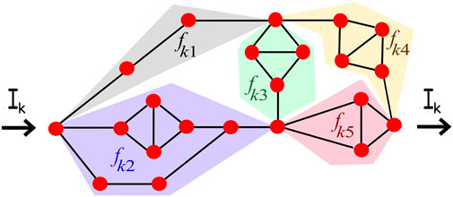
FIGURE 3. Recovering the currents in a typical 3-connected component of level k through which passes a current I_k. After its internal 3CCs have been replaced by effective bonds, this component turns into a simple Wheatstone bridge that can be readily solved to obtain the fraction f_ks of the current I_k passing through each segment s of the Wheatstone bridge. The current of every bond in segment s is then reduced in level k by this factor f_ks. We consider two different ways of sampling the factors f_ks. In the first sampling, we count the so-called actual bonds of level k. These are bonds in segment s that are inside level k but outside level k + 1. In the second sampling, we count the internal bonds, namely, all other bonds in the segment s that are not actual bonds of level k, that is, any bond in s found inside 3CCs of level k + 1. In this example, the factor f_k1 is sampled three times in the distribution for actual bonds and is not included in the distribution for internal bonds as there are no 3CCs in this segment. The factor f_k5 is sampled five times in the distribution of internal bonds and is not included in the distribution of actual bonds as there is no bond carrying the whole current passing through this segment. The factor f_k2 is sampled 10 times by internal bonds and just one by actual bonds.

FIGURE 4

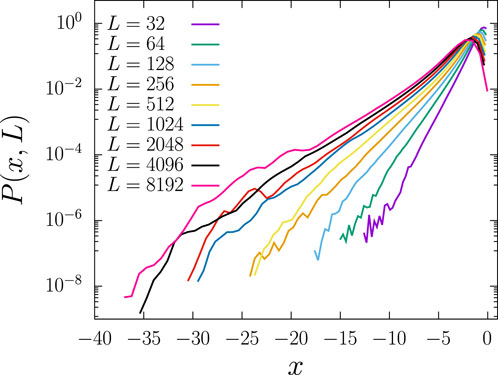
FIGURE 4. Current distribution on critical conducting backbones for different system sizes L × L. In this graph, x = log₁₀(i_ℓ), with i_ℓ, being the currents in each bond. The results were obtained for square lattice subjected to bond percolation at the critical point p_c = 1/2. For each size, we simulated at least 2,000 samples. For each sample, we recovered the largest cluster, applied a potential difference at a pair of nodes separated by L/2 lattice units, and extracted the backbone [22]. Our approach allows obtaining with precision currents of the order of 10⁻³⁵.

2.1 Distribution of current factors

At this point, we make use of our method to study the distribution of the multiplying factors, f_ks. In order to fully describe their statistics, two different sampling ways are adopted, as shown in Figure 3. In the first way, a factor f_ks is sampled by the number of actual bonds of level k in segment s. A bond is of level k when it is inside level k but outside level k + 1. Alternatively, we sample the same factor f_ks by the number of internal bonds. The internal bonds correspond to all other bonds in segment s that are not actual bonds, namely, all bonds in the segment s that are nested inside 3CCs of level k + 1 or higher.

As shown in Figure 5, the distributions of factors generated in both sampling ways closely follow power-law behavior, P(f) ∼ f^α, for over more than seven orders of magnitude. Moreover, the least-squares fits to the datasets of this power-law for all levels k give similar exponents that, within the statistical error bars, are consistent with the value α = 3/4. Approaching the limit f = 1, all distributions above level k = 0 display an exponential cut-off to a vanishing probability. This is to be expected since inside a 3CC, there are no bonds carrying the whole current. For k > 1, the distributions appear to be independent on the level. Level 0 contains the so-called red bonds that carry the total current. For bonds at level 0, very few bonds have f ≠ 1, indicating that only a very small fraction of the blobs consists of parallel bonds, like the ones present in the hierarchical model, as shown in the inset of Figure 2.

FIGURE 5

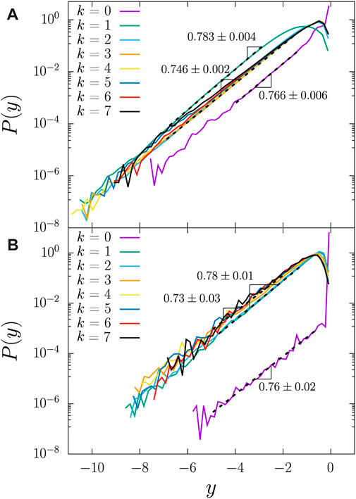
FIGURE 5. Distribution of factors for each level k of the hierarchical structure of the conducting backbone at the critical bond percolation point, p_c = 1/2. In this graph, y = log₁₀(F), with f being the factor by which the currents are reduced when split inside a given 3CC. These results were obtained from numerical simulations using 10,000 realizations of two-dimensional square lattices with size L = 2048. In (A), we show the distribution of factors for actual bonds, and in (B), the distribution for factors on effective bonds. As explained in the main text and in the caption of Figure 3, both distributions are obtained from the same set of factors but with different sampling weights. The distributions closely follow power laws, P(F) ∼ f^α, over up to seven orders of magnitude with exponents that are consistent with the value α = 3/4. Except for k = 0, they all display an exponential cut-off in the proximity of f = 1. Within the statistical fluctuations, the tail of the curves falls on top of each other for k > 1.

Since from level 1 upwards factors are strictly smaller than unity and higher levels correspond to a multiplication of more factors, the current distribution for bonds of higher levels should move toward smaller values. This is confirmed in Figure 6, where we present the current distributions separated by the bond level. The curves move toward weak currents by over one order of magnitude per level, becoming less skewed.

FIGURE 6

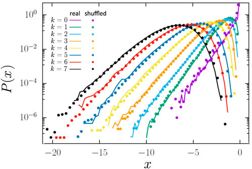
FIGURE 6. Current distribution segregated by the bond level. In this graph x = log₁₀(i_ℓ), with i_ℓ being the currents in a given bond. The solid lines correspond to the current distributions on the bonds within a given level k. As expected, the bonds at higher levels tend to carry a smaller fraction of the total current. In order to test for the presence of correlations between values of factors at different levels, we also generate current distributions from randomly shuffled data (dots). As can be seen, the shuffled data follow closely the numerical results, suggesting that the factors at different levels are statistically independent.

In order to see if there are correlations between factors of different levels, we also compute the distributions after randomly shuffling the data. Precisely, we construct a shuffled current of level k in the following way. Precisely, to construct a shuffled current of level k, for each level from 0 to k − 1, we chose randomly a factor from the distribution of factors for internal bonds (Figure 5B), while for the level k, we chose randomly a factor from the distribution of factors for actual bonds (Figure 5A). As can be seen in Figure 6, the distributions for the shuffled data follow closely the distributions obtained for the real current, suggesting that factors at each level are drawn from independent distributions. The current distribution of the whole network should be obtained by summing the expected distributions for each level weighted by the fraction of bonds of each level in the backbone.

2.2 Distribution of hierarchical levels

Figure 7 shows that the distributions of bond levels k display exponential decays for sufficiently large values of k, indicating that the appearance of a 3CC is a Poissonian process. Moreover, the larger the system size L, the less abrupt the decay becomes. As shown in the main panel of Figure 7, for k ≠ 0, this size dependence is suppressed for levels at the interval 1 ≤ k ≤ 10 when both axes are re-scaled by a factor L^θ, where the exponent θ = 0.16 ± 0.01. The fraction of bonds in level 0 systematically decreases with system size like $L^{-5/4}=L^{d_r-2}$, where d_r = 1/ν = 3/4 is the fractal dimension of the red bonds [23].

FIGURE 7

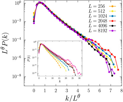
FIGURE 7. Distribution of bond levels k. As shown in the main panel, the distribution of levels seems to obey a scaling relation since the variable k/L^θ, with θ = 0.16 ± 0.01, allows collapsing the data for all system sizes. Some deviation at the tail of the distribution is most likely due to fluctuations resulting from the small frequency of extremely small currents. It should be noted, however, that the same scaling does not hold for bonds of level 0, which seem to collapse with an exponent consistent with 3/4 (not shown). In the inset, we show the distribution without rescaling the axis.

3 Discussion

By exploiting the self-similarity of a critical percolation backbone, we disclosed a hierarchical structure in its 3-connected components, which ends up allowing an extremely efficient decomposition of the whole system. Level 0 of this hierarchy corresponds to bonds that are just in series or in parallel, and their number increases with system size like the red bonds. The occupancy of higher levels follows a Poisson distribution scaling with the fractal dimension of 3CCs, while the fractions of the current at each level are power-law-distributed with exponents consistent with the value 3/4. Finally, through data reshuffling, we showed that the distributions of factors for internal and actual bonds are uncorrelated. In this way, the complex finite-size behavior of the current distribution can be recovered by multiplying factors randomly drawn from their power law distributions, according to the Poisson distribution of levels.

Another important outcome of our work is the development of a very efficient solver for the local currents in the critical backbone. We also implemented our algorithm on triangular and hexagonal lattices obtaining the same scaling relations and exponents observed for the square lattice. The generalization of our algorithm to higher dimensions is straightforward, and we are presently working on three-dimensional lattices.

Our new way of evaluating current distributions on fractal graphs and the huge gain in precision that we could achieve with this method will allow not only to gain insights on the multifractality of percolation clusters, as shown in the present work, but also to analyze with higher precision than before, for instance, traffic on sparse networks, fluid flow in capillary systems, or the effect of weak bonds in incipient gels.

Data availability statement

The original contributions presented in the study are included in the article/Supplementary material; further inquiries can be directed to the corresponding author.

Author contributions

WS: writing–original manuscript and writing–review and editing. JA: writing–original manuscript and writing–review and editing. HH: writing–original manuscript and writing–review and editing. AM: writing–original manuscript and writing–review and editing.

Funding

The author(s) declare financial support was received for the research, authorship, and/or publication of this article. The authors thank the Brazilian agencies CNPq, CAPES, FUNCAP, the National Institute of Science and Technology for Complex Systems of Brazil (INCT-SC), Petrobras (“Física do Petróleo em Meios Porosos,” Project Number: F0185), and the PRONEX-FUNCAP/CNPq Award PR2-0101-00050.01.00/15 for financial support.

Conflict of interest

The authors declare that the research was conducted in the absence of any commercial or financial relationships that could be construed as a potential conflict of interest.

The author(s) declared that they were an editorial board member of Frontiers, at the time of submission. This had no impact on the peer review process and the final decision.

Publisher’s note

All claims expressed in this article are solely those of the authors and do not necessarily represent those of their affiliated organizations, or those of the publisher, the editors, and the reviewers. Any product that may be evaluated in this article, or claim that may be made by its manufacturer, is not guaranteed or endorsed by the publisher.

References

1. Broadbent SR, Hammersley JM. Percolation processes: I. Crystals and mazes. Proc Cambridge Phil Soc (1957) 53:629–41. doi:10.1017/s0305004100032680

CrossRef Full Text | Google Scholar

2. Stauffer D, Aharony A. Introduction to percolation theory. United Kingdom: Taylor & Francis (1992).

Google Scholar

3. Kirkpatrick S. Classical transport in disordered media: scaling and effective-medium theories. Phys Rev Lett (1971) 27:1722–5. doi:10.1103/physrevlett.27.1722

CrossRef Full Text | Google Scholar

4. Sahimi M. Flow and transport in porous media and fractured rock. United Kingdom: John Wiley and Sons (2011).

Google Scholar

5. Hunt AG, Ewing R, Ghanbarian B. Percolation theory for flow in porous media. Lecture Notes Phys (2014) 771. doi:10.1007/978-3-319-03771-4

CrossRef Full Text | Google Scholar

6. Andrade JS, Street DA, Shinohara T, Shibusa Y, Arai Y. Percolation disorder in viscous and nonviscous flow through porous media. Phys Rev E (1995) 51:5725–31. doi:10.1103/physreve.51.5725

PubMed Abstract | CrossRef Full Text | Google Scholar

7. Andrade JS, Almeida MP, Mendes Filho J, Havlin S, Suki B, Stanley HE. Fluid flow through porous media: the role of stagnant zones. Phys Rev Lett (1997) 79:3901–4. doi:10.1103/physrevlett.79.3901

CrossRef Full Text | Google Scholar

8. King PR, Andrade JS, Buldyrev SN, Dokholyan N, Lee Y, Havlin S. Distribution of shortest paths in percolation. Physica A: Stat Mech its Appl (1999) 266:55–61. doi:10.1016/s0378-4371(98)00574-3

CrossRef Full Text | Google Scholar

9. King PR, Masihi M. Percolation theory in reservoir engineering. Singapore: World Scientific (2018).

Google Scholar

10. Tremblay AMS, Fourcade B, Breton P. Multifractals and noise in metal-insulator mixtures. Physica A (1989) 157:89–100. doi:10.1016/0378-4371(89)90282-3

CrossRef Full Text | Google Scholar

11. de Arcangelis L, Redner S, Coniglio A. Anomalous voltage distribution of random resistor networks and a new model for the backbone at the percolation threshold. Phys Rev B (1985) 31:4725–7. doi:10.1103/physrevb.31.4725

CrossRef Full Text | Google Scholar

12. Barthelemy M, Buldyrev SV, Havlin S, Stanley HE. Fractals (2003) 11:19–27. doi:10.1142/s0218348x03001689

CrossRef Full Text

13. Batrouni G, Hansen A, Roux S. Negative moments of the current spectrum in the random-resistor network. Phys Rev A (1988) 38:3820–3. doi:10.1103/physreva.38.3820

PubMed Abstract | CrossRef Full Text | Google Scholar

14. Aharony A, Blumenfeld R, Harris AB. Distribution of the logarithms of currents in percolating resistor networks. I. Theory. Phys Rev B (1993) 47:5756–69. doi:10.1103/physrevb.47.5756

PubMed Abstract | CrossRef Full Text | Google Scholar

15. Barthelemy M, Buldyrev SV, Havlin S, Stanley HE. Multifractal properties of the random resistor network. Phys Rev E (2000) 61:R3283–6. doi:10.1103/physreve.61.r3283

PubMed Abstract | CrossRef Full Text | Google Scholar

16. Hopcroft JE, Tarjan RE. Dividing a graph into triconnected components. SIAM J Comput (1973) 2:135–58. doi:10.1137/0202012

CrossRef Full Text | Google Scholar

17. Gutwenger C, Mutzel P. Int. Symp. On graph drawing. Berlin, Germany: Springer (2000). p. 77.

Google Scholar

18. Paul G, Stanley HE. Beyond blobs in percolation cluster structure: the distribution of 3-blocks at the percolation threshold. Phys Rev E (2002) 65:056126. doi:10.1103/physreve.65.056126

PubMed Abstract | CrossRef Full Text | Google Scholar

19. Herrmann HJ, Stanley HE. Building blocks of percolation clusters: volatile fractals. Phys Rev Lett (1984) 53:1121–4. doi:10.1103/physrevlett.53.1121

CrossRef Full Text | Google Scholar

20. de Arcangelis L, Redner S, Coniglio A. Multiscaling approach in random resistor and random superconducting networks. Phys Rev B (1986) 34:4656–73. doi:10.1103/physrevb.34.4656

CrossRef Full Text | Google Scholar

21. Rintoul MD, Nakanishi H. A precise determination of the backbone fractal dimension on two-dimensional percolation clusters. J Phys A (1992) 25:945–8. doi:10.1088/0305-4470/25/15/008

CrossRef Full Text | Google Scholar

22. Hopcroft J, Tarjan R. Algorithm 447: efficient algorithms for graph manipulation. Commun ACM (1973) 16:372–8. doi:10.1145/362248.362272

CrossRef Full Text | Google Scholar

23. Coniglio A. Cluster structure near the percolation threshold. J Phys A (1982) 15:3829–44. doi:10.1088/0305-4470/15/12/032

CrossRef Full Text | Google Scholar