 Biao Wang
 Yan Huang
 Yongyue Yang1
 Yonghong Wang
- 1School of Instrument Science and Opti-Electronics Engineering, Hefei University of Technology, Hefei, Anhui, China
- 2Intelligent Equipment Department, Zhejiang Jiashan Shuangfei Lubricant Material Co., Ltd., Jiashan, Zhejiang, China
Automatic defect-detection technology based on deep learning is increasingly used for distinguishing production quality by many industries. However, production lines are usually installed with lots of function modules, which make it difficult to integrate new modules. Common deep learning models run on PC platforms and require a big space with high cost, while ARM64 mobile platforms are much smaller with less cost and equivalent connectivity but also weaker performance. Considering these facts, ARM64 platforms with a fully optimized model are the best solution for adding a defect-detection function for existing production lines. This paper focused on a mobile-optimized model to achieve higher speed and equivalent precision on the ARM64 mobile platform for detection. First, the model structure is simplified by reducing the redundancy of feature maps to increase the network inference speed. Second, a convolutional block attention module is attached to compensate for the decrease in precision caused by structure simplification. Furthermore, a transfer learning method is adopted to improve training performance. Finally, the trained and compiled module is exported to the PyTorch Mobile format and deployed on the mobile platform application to execute its defect-detection function. The results show that the optimized network achieves a speed of 2.124 fps, 210.7% compared with that of You Only Look Once v5n, i.e., 1.008 fps, on the RK3399 ARM64 platform, and has an average mAP of 99.2%. The studied mobile-optimized model has better speed and equivalent precision and can be available on many different ARM64 platforms regardless of the processor manufacturer. It can satisfy the need for real-time defect detection and can be used in similar scenarios. In the future, more improvements could be made such as deploying on platforms with NPU support to achieve faster speed, exploring the relationships between dataset properties and transfer learning effects, even training and running the model directly on ARM64 platforms.
1 Introduction
With the advance of industrial automation technology, an increasing number of different functional modules have been attached to the production line. These modules take individual areas in a limited space, but integrating them into one system would be difficult, which limits the application of new modules.
Meanwhile, automatic production quality control demands an effective defect-detection method, as defect detection is an important quality control method in many fields like industry, agriculture, and medicine. Deep learning-based machine vision could be a good choice with its adaptivity of different target objects without programming a complex algorithm. Considering the needs of a defect-detect function and space limit for new modules, a small-size deep learning-based defect-detection module is the best for adding such a function to the existing production line.
The defect-detection module consists of software (deep learning-based application) and hardware (deployment platform). Regarding the hardware, which determines the space occupied, a traditional industry PC can run the application with good speed and precision but needs large space and cannot be shared with different modules, which make it difficult for production line deployment.
Different from PCs, newly developed ARM64 hardware platforms are much smaller with equivalent extensibility, owing to the long-term evolution of ARM architecture. The popularity of mobile phones accelerated the ARM evolution speed, enabled a high-performance core design, and brought in a platform with numerous hardware applications and well-optimized operating system support. Nowadays, ARM64 platforms are good enough for running industrial controlling systems, with their small size and low cost, as well as valid hardware and software ecology. Some deep learning frameworks, like PyTorch Mobile and TensorFlow Lite, are developed for mobile platforms, which can be used for creating deep learning-related applications. These factors show the feasibility of developing a deep learning defect-detection application on ARM64 mobile platforms.
However, the ARM64 platforms are much slower than PC platforms due to weaker processor performance and the absence of discrete GPU support. So, the models which run on a PC smoothly could be very slow on an ARM64 platform due to large model size. Therefore, it is necessary to design a lightweight model which could run on an ARM64 platform with fast inference speed. In addition, the industrial defect detection also demands the model to have good precision as missing too many defects is unacceptable.
In this article, the design of a lightweight defect-detection model for a composite plate is presented. A composite plate is a kind of material based on metal, with an added coating material for acquiring special surface properties. The composite plate is then used to create oil-free lubrication bearings, and the performance of the bearing is determined by the plate-coated surface quality. Therefore, the automatic defect detection of the plate surface is very important.
The manufacturing procedure is simple but liable to produce defects on the plate surface. First, the loading system loads a solid coating material on the base board, where impurities may be contained by the material. The board with a coating material is then preheated with hot nitrogen gas and pressed using a hot rolling wheel to melt and flatten the coating material on the base board. As shown in Figure 1, the manufacturing procedure is full of heating and pressing, which could be affected by temperature and pressure differences. Figure 2 shows a color image sample of a defect on a composite plate. Obviously, the dark dot area is a defect. Defects on the surface could cause serious problems because of their effect on the physical characteristics of the surface, like friction coefficient. Bearings with defects wear out quickly and even cause more damage. Additionally, the composite plate production environment could become very hot because of the heating devices. Furthermore, numerous controlling devices require much space, and little space is left for new modules in the production line.
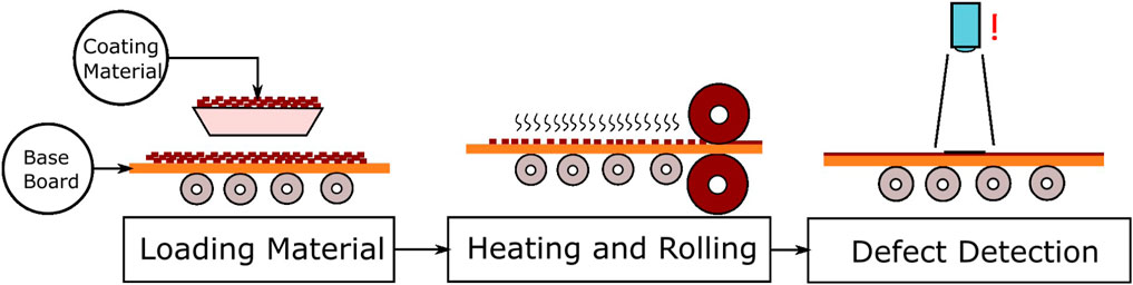
FIGURE 1. Composite plate manufacturing procedure.
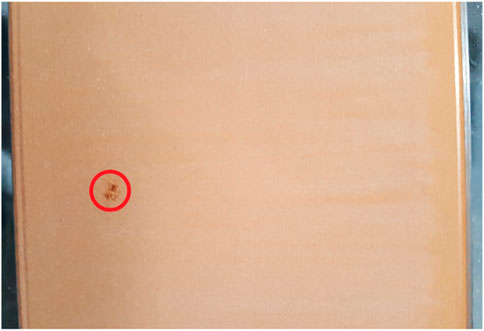
FIGURE 2. Composite plate defect color image sample. The dust in the red circle is a defect.
Therefore, to add an automatic defect-detection function for existing production lines, using a space-saving ARM64 platform with a defect-detection model is a good choice. However, there are problems that need to be solved for model deployment. First, common models are designed for running on a PC platform with large-scale and complex structures, making them run very slowly on ARM64 platforms. Second, simply cutting the model structure could make it run faster but decreases precision significantly, which is unacceptable for industrial use. Last, the datasets for industrial defect-detection purposes are not as abundant as common datasets, like PASCAL VOC and MS COCO series, while they are collected by the industry user for defect detection of specified products. So, the effect of dataset insufficiency should be considered.
Thus, this study proposed a defect-detection deep learning model based on You Only Look Once (YOLO) v5n and processed its deployment on the ARM64 platform. The following efforts were made:
1. The model structure is simplified with Ghost Reduced (GR)-Stem and Asymmetric Ghost Reduced (AGR)-Downsampling blocks, which contained Ghost modules to reduce redundancy, making it much lighter and faster than many object-detection models. Ghost modules use base feature maps with cheap operation to generate similar feature maps, and the redundant parameters for expressing complete feature maps could be reduced. The comparison and analysis are explained in Section 4.2.
2. The model inserted a convolutional block attention module (CBAM) to compensate its precision without much speed and size cost. Although the model is much smaller after simplification, its feature extraction ability is also weaker than before. An attention mechanism could let the model pay more attention and strengthen feature extraction on the target area. The effectiveness analysis is explained in Section 4.3.
3. The model is trained with a transfer learning method to improve its retrain performance. As LED and composite plate defect-detection tasks are similar, a transfer learning method can be deployed. By using an LED defect dataset with abundant defect images, we can fully train the model to perfect its structure and generate an available pre-trained weight. Then, the model is retrained with a composite plate defect dataset to achieve its target function, as well as faster training speed and further improvement in precision, due to a previous pre-train procedure with the LED defect dataset. Details are provided in Section 3.1.4, Section 4.3.
4. The model is deployed as a PyTorch Mobile application and tested on the ARM64 platform. The manufacturer’s support, like NVIDIA mobile GPU and CUDA, is not essential, which makes it easy to use on various ARM64 platforms with Android OS support. Its wide applicability makes it practical for industrial use and provides valuable data for further research. The deployment procedure and test results are given in Section 3.2, Section 4.3.
2 Related work
Scholars worldwide work on automatic object detection and put forward many algorithms and deep learning models with the development of information technology. For example, Mordia and Kumar Verma [1] concluded on a possible way for defect detection in steel products, which are similar to composite plates. A machine vision algorithm could be a possible choice for automatic defect detection. However, it is difficult to design because of the difference between distinct baseboards and defect features. Changing while loaded on the hardware system is difficult, and adapting to possible situations is even more difficult. Therefore, the convolutional neural network (CNN) is a better choice because of its adaptability and precision. For deep learning methods, Wang et al. worked on LED defect detection with Faster R-CNN and achieved an overall accuracy of 95.6% with approximately 10 fps on a high-performance PC platform [2]. Wang et al. used YOLOv5n for detecting apple stem/calyx and arrived at an average precision of 93.89% on the apple image datasets acquired [3]. Deep learning-related CNN models are good for studying defect features without manually modifying procedures, and pertinent optimization could encounter the disadvantage of execution speed.
Regarding the defect-detection purpose, we could use detector algorithms as well as deep learning models. Furthermore, the models could be divided into two kinds: two-stage models and one-stage models. The progress made by researchers is presented in the following sections.
2.1 Detector algorithm methods
Traditional detection methods are the beginners of automatic object detection, and the initial target was human detection. Paul Viola and Michael Jones created the Viola–Jones object-detection framework by combining many different technologies like Haar-like feature, integration image, and AdaBoost detector and classifier [4]. Dala and Triggs put forward the HOG algorithm to extract boundary gradients and their direction to create the feature list [5]. In 2009, Felzenszwalb developed the DPM algorithm which detects different parts of the target from the whole image and removes irrelevant areas to produce final detection results [6].
2.2 Two-stage models
With the evolution of deep learning, two-stage models came into existence, which include R-CNN, Fast R-CNN, Faster R-CNN, and SPP-Net. The R-CNN series are one of the famous object-detection models. They use selective search methods to find proposal regions and support vector machines (SVMs) to determine whether the region includes the target. Girshck et al. put forward an R-CNN model [7] first and improved it continually, and then came out with Fast R-CNN [8], SPP-Net [9], and Faster R-CNN [10]. Faster R-CNN uses VGG16 as the backbone of feature extraction and combines RPN and Fast R-CNN ideas. Affected by the structure, two-stage models are slower with more precision than one-stage models generally [11].
2.3 One-stage models
Different from two-stage models, one-stage models extract characteristics and detect the target directly, which makes them faster than two-stage models but with lower precision. It is better to deploy one-stage models on the ARM64 platform to achieve real-time defect detection.
2.3.1 YOLO series
As one of the most popular object-detection deep learning networks, the YOLO series network has a higher detection speed than others. Redmon et al. designed YOLO, YOLO9000, and YOLOv3 networks [12–14]. The modified version of these networks is also uncountable, like YOLOv3-tiny and YOLOv3-dense, and the authors attempted to optimize the network speed and size. Zhang created an improved YOLOv3-tiny pedestrian detection model with a detection speed of 4.84 ms on the GPU [15]. After Redmon stopped working on YOLO’s further development, Bochkovskiy et al. designed YOLOv4 based on Redmon’s work [16]. Currently, YOLOv5 is being created by Ultralytic and Alexey Bochkovskiy, as PyTorch and TensorFlow versions [17]. However, the precision of YOLO is affected when detecting small-sized targets, which is determined by its one-stage characteristic. Pham et al. put forward the YOLO-Fine network to improve the small target detection performance [11].
2.3.2 MobileNet series
To increase network speed, simplification is necessary. The original YOLOv5 used Darknet-53 as a backbone, but it is too heavy for a light network. The MobileNet series came out with a good start [18,19]. Chen et al. used attention-embedded MobileNetV2 to identify crop diseases and obtained an average accuracy of 99.13% [20].
2.3.3 ShuffleNet series
Furthermore, ShuffleNet simplified the network, improved accuracy, and increased speed [21,22]. Huang and Lin performed breast density classification using ShuffleNet and achieved lesser time for model training and running [23]. Based on improved ShuffleNet v2, Chen et al. built a garbage classification system and created 105-ms single-inference time on Raspberry Pi 4B [24].
2.3.4 PeleeNet series
PeleeNet obtained a new angle for decreased network size [25]. With a cost-efficient stem block before the first dense layer, the feature expression ability improved without adding too much computational cost, which is important for maintaining precision with a small network structure. For example, Piao et al. used PeleeNet as the backbone network of their model to speed up the inference and obtained better results than SSD in terms of detection accuracy and detection speed [26].
2.4 Model enhancement
Regarding model design, scholars work on developing functional blocks or methods to improve deep learning model performance without any major changes to the structure.
2.4.1 Function module developing
Simplification and speed increase for models can also be achieved by using a specialized function module. Huawei put forward the Ghost module, which achieved good speed improvement results on many baseline models [27]. By transforming a feature map into another map through cheap operations, fewer parameters and floating point operations are used in the model. As shown in Figure 3, some similar feature maps are generated by ResNet-50 and our model.
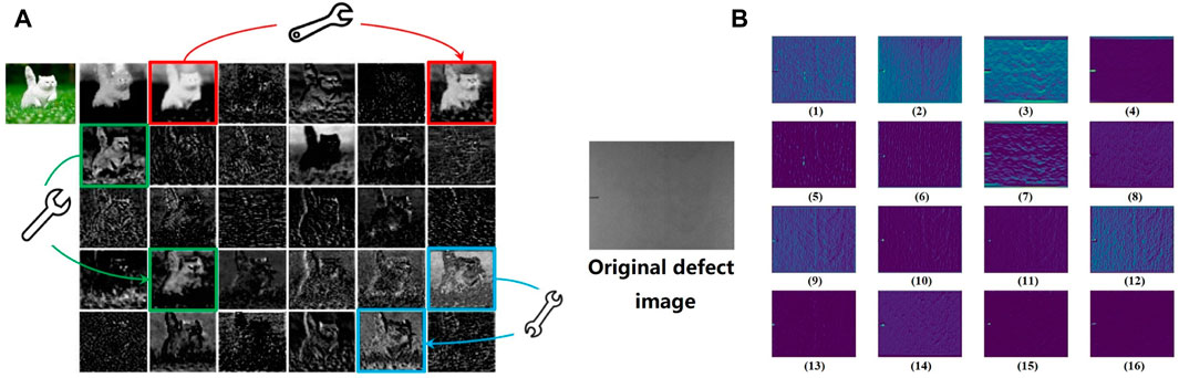
FIGURE 3. (A) Visualization of some feature maps generated by the first residual group in ResNet-50, with three similar feature map pair examples annotated with boxes of the same color [27]. (B) Visualization of feature maps generated by the GR-Stem block. Images 1 and 2, 3 and 7, and 9 and 12 are similar.
In Figure 4, the Ghost module uses base feature maps and cheap operations to generate similar feature maps instead of using a complete feature map, which could reduce lot of redundancy produced by similarity.
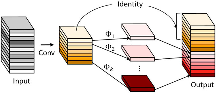
FIGURE 4. GhostConv structure. ϕ means cheap operation [27].
For enhancing detection precision, an attention structure is a good idea, and many researchers have worked on it. The squeeze-attention network is the forerunner that puts forward a structure with the squeeze-excitation attention module [28], and Deng et al. applied the module on original networks, like Inception-V4, ResNeXt, and DenseNet, and obtained a significant performance increase in breast density image detection [29]. Then, the block attention module and convolutional block attention module were created with better performance [30,31]. The CBAM can be used in prohibited item detection in X-ray images to improve performance [32]. Meanwhile, other ways exist to add attention structure to CNNs. For example, the CAT-CNN put forward by Liao et al. performed attention enhancement with different kinds of CNNs and obtained satisfying results [33]. Yang et al. tested the performance of different attention structures on a YOLOv5-based model for invasive plant seed detection [34].
2.4.2 Transfer learning
Transfer learning is a good method to improve the performance of a model without changing the model structure. The idea of transfer learning was inspired by human learning behavior, where humans use previous related knowledge while learning to solve new problems. Transfer learning enables machine learning models to transfer learned knowledge from source domains to a target domain to improve the performance of the target learning function while both the source and target domain have different data distributions. Jamil et al. used a deep boosted transfer learning method to check wind turbine gearbox faults [35]. Zitong Wang et al. reviewed transfer learning methods in electroencephalogram (EEG) signal analysis, like domain adaptation, improved CSP algorithms, DNN algorithms, and subspace learning [36]. Generally, transfer learning is an efficient way for improving model performance without extensive structure modification.
2.5 Summary
In our study, to achieve defect detection on the ARM64 mobile platform, a one-stage network is a good base but needs proper design to make it lightweight and precise. First, most of the deep learning networks are designed for computer platforms with GPU acceleration. Thus, they need to be simplified for mobile platforms. After studying newly developed mobile-optimized deep learning networks, some structures of existing networks are worth importing as a replacement. The backbone area is involved in the characteristic extraction, and it costs the majority of the calculation quantity. Therefore, the backbone should be focused on simplification. Second, shrinking the model size would decrease its precision and training speed because its characteristic extraction is affected by decreased size. Consequently, compensation measures should be taken to maintain precision. Finally, when YOLOv5 was tested to run directly on Ubuntu or Debian ARM64 with a PyTorch ARM64 port, it returned an illegal instruction error. Furthermore, PyTorch Mobile is easier for application programming with Android OS support. So, we chose PyTorch Mobile (PyTorch open-source project, 2022a) instead of PyTorch as a framework for running the network on the ARM64 platform.
3 Network design and optimization
The model structure is shown in Figure 5, and network developing contents are mentioned in the following sections.
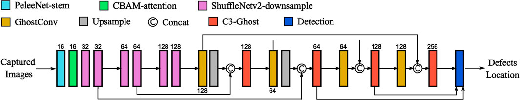
FIGURE 5. CPDD-CLMM network structure.
3.1 Efficiency focused
As mentioned in a previous paper, redundant feature maps could be expressed by one basic feature map with relative parameters. For example, the baseline YOLOv5 backbone is made from Darknet-53, which started from YOLOv3. It evolved from Darknet-19 in YOLOv2, with more shortcut connections and larger scales [14]. However, the Darknet-53 structure is still too large for a lightweight model with its redundancy on mobile platforms. Thus, we create a simplified backbone structure with designed blocks to decrease size and increase speed. Block structures are shown in Figure 6A.
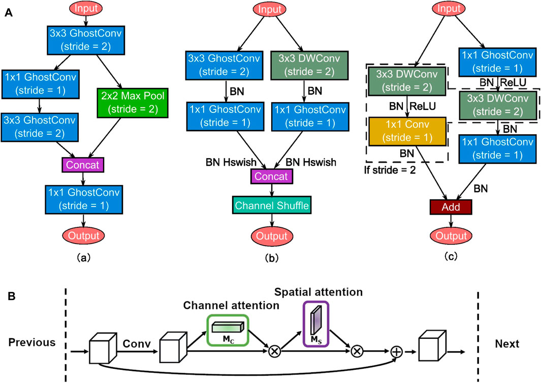
FIGURE 6. (A) GR (Ghost Reduced)-Stem module (a), AGR (Asymmetric Ghost Reduced)-Downsampling module (b) and C3-Ghost (c). DWConv: depthwise convolution. BN, batch normalize. (B) CBAM structure.
The GR-Stem block could improve the feature expression without adding computational complexity. The AGR-Downsample blocks act as the main characteristic extractors with Hard Swish activation function. Tensor padding is one, which means filling one at the boundary of matrix. The module could extract features with GhostConv and DWConv to reduce redundancy and maintain different features acquired by two branches. The block channel shuffle structure is useful for collecting information from different channel mix ups and establishing connections. Although the images appear to be in gray scale, they are in RGB format with multiple color channels. Therefore, it is necessary to use channel shuffle to mix up information from different channels, and it provides compatibility for color camera input. It works as feature pyramid networks, when the neck works as path aggregation networks. Ghost reduced means using Ghost convolution to reduce redundancy for both kinds of blocks. The backbone size became much smaller by using these modules.
The neck and head structures work as one-stage object detectors, making them faster than two-stage models which need multiple procedures of region proposals [11]. In the neck structure, C3-conv is a bottleneck block included by the original YOLOv5n model for preserving spatial dimensions and reducing network depth. However, it is still expensive. We use C3-Ghost instead to simplify the structure and improve speed. The detection block, which is regarded as the head, executes to generate a bounding box for the target.
3.2 Maintaining precision
After optimization of efficiency, the network is much faster but has lower precision. The CBAM combined spatial and channel attention and made it better than SANet which only obtained channel attention enhancement. Its structure is shown in Figure 6B. The intermediate feature map is adaptively refined through the attention module at every convolutional block of deep networks. The module is placed behind the stem module to apply its function.
Transfer learning is an effective method to improve model performance. By training a more complete dataset which is relative to the target dataset, the model could learn and establish a structure. Then, the model is trained with the target dataset, which makes the model faster and perform better than when trained with the target dataset directly.
The defects that appear on the composite plate surface are deeper than in the normal area and have a clear boundary, which makes their features relatively simple and similar, even though we attempted to augment it by adding noise, rotating, or adjusting the brightness and contrast. However, LED defects are different and much more complex. For example, the air bubble defects in LED are multiplex with different sizes and color features. Therefore, the LED defect dataset is suitable for transfer learning of our model, with the same task goal of defect detection but more difficult, which is good for the model to generate its structure.
The model is trained with the LED defect dataset to generate pre-trained model weights. The dataset was provided by Yalan Zhou, with 1788 different images of defects, like air bubbles [2]. The dataset sample is shown in Figure 7. Then, pre-trained weights are imported, and a composite plate dataset is used to make the model available.
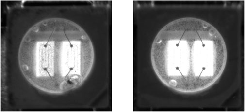
FIGURE 7. LED defect dataset sample.
3.3 Training without refined tuning
The model designed needs more training epochs to obtain enough precision considering its small size, so we set the maximum training epoch limit as 2,000 epochs with a batch size of 16. The pre-trained weight file of YOLOv5n is downloaded from Ultralytics’ GitHub as the training method dependency. The model is trained on a PC platform with an Intel Core i7-10850K CPU and NVIDIA RTX3090 GPU, and CUDA acceleration is enabled for maximum training speed. Warmup and fine-tune training techniques are applied to enhance the training procedure, with YOLOv5 “scratch” hyperparameter settings and SGD optimizer enabled. The fine-tuning of hyperparameters could take a significant amount of time, which is not beneficial for field engineers to deploy the model. Therefore, we use original YOLOv5 hyperparameters, focusing on the structure and training optimization. Hyperparameters are shown in Table 1.
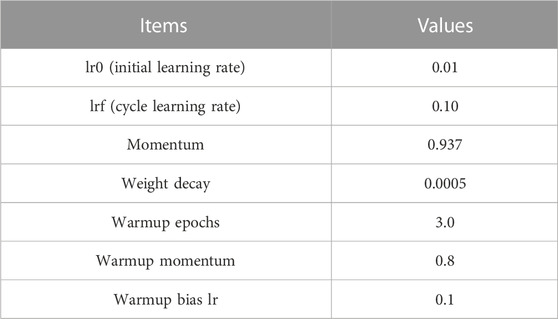
TABLE 1. Model hyperparameters.
3.4 Mobile platform testing
The chart of deploying CPDD-CLMM on the ARM64 platform is given in Figure 8A. The model will be a part of the defect-detection application with PyTorch Mobile runtime. PyTorch Mobile is a runtime for deploying a deep learning model on mobile devices while staying entirely within the PyTorch ecosystem. It does not rely on specific functions like CUDA, which is only available on a specified manufacturer’s product. It has good compatibility with different platforms and is a good choice for running a deep learning model on embedded ARM64 processors. A demo app for object detection is available on the PyTorch Mobile GitHub website, which is the best start for deploying the modified model on the Android ARM64 platform, instead of creating a new app. The application controls the capture camera to gather images, and CPDD-CLMM processes them to find out the defects. The results could be uploaded to monitor for further actions with wired or wireless network connection.
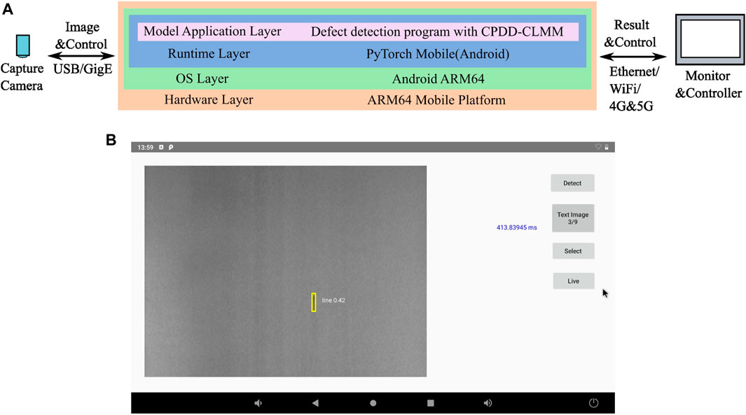
FIGURE 8. (A) Deployment chart of CPDD-CLMM on ARM64 platform and (B) defect detection application interface.
The screenshot of the defect-detection app is shown in Figure 8B. The normal orientation of the demonstration is portrait suitable for mobile phones. To make full use of the screen, the orientation is changed to landscape (Figure 8B). Deployment procedures are explained as follows.
First, the model is trained with a common procedure in a Python environment, and the GPU can be used for acceleration. Second, export.py provided by YOLOv5 is used with necessary instructions to convert the output model file into PyTorch Mobile format (PyTorch open-source project, 2022b). As a runtime framework, PyTorch Mobile could only run a just-in-time (JIT)-translated CNN model. The model file output in the first step is in .pt format without PyTorch Mobile optimization, which cannot be used for app creation. Therefore, the instruction listed on PyTorch Mobile GitHub should be followed to make the model available. Third, the translated model is placed in the app source folder, the corresponding model filename is changed in the source code, and the application is compiled. Fourth, the application package is installed on the system. Last, the model is deployed on the Android ARM64 platform and made available for detection.
The output data are an array containing seven attributes as bounding box upper-left corner (X, Y) coordinates, bounding box width and height, confidence score, and classification probabilities. The number of initial bounding box outputs by the original model is (20*20 + 40*40 + 80*80) * 3 = 25,200, where the multiplied part corresponds to different bounding box groups and 3 denotes three groups. The original YOLOv5 model input image size 640*640, and we can obtain the 20*20 block if the downsample size is 32, with (640/32) * (640/32) = 20*20. For the proposed model, the formula is (20*15 + 40*30 + 80*60) * 3 = 6,300, with an input image size of 640*480. Finally, the output of the generated bounding box array size is 6,300 (boxes) * 7(attributes) = 44,100. An overflow error would occur if the row size is unchanged with the modified model imported.
To measure the model performance, the average inference time is used and defined as the time taken for processing different testing images, and a timer is needed because the demo provided does not include a timer. A timer is then added to the app’s main interface (Figure 8B). Java provided two methods, “System.currentTimeMills()” and “System.nanoTime(),” for time measurement and described their details in the Java SE 17 API documentation [37]. We chose nanotime function to provide nanosecond precision. The application runs in the Android ART Java virtual machine, and the time resolution is affected by the hardware and system kernel time fresh rate. To make the measurement as precise as possible, the inference time counter starts at the beginning of the inference thread and stops at the beginning of the result output. The app can detect defects from images or camera video streams. For speed-testing purposes, an image detecting method is used to obtain the average time the model takes for inferencing a result.
Two platforms were prepared to test the models with different performance levels (Table 2). The main target platform is the Rockpi 4b+ with Rockchip RK3399 as a good standard of an industrial- and commercial-grade ARM processor. Alongside the RK3399 platform, the SM8250-AC (Qualcomm Snapdragon 870) platform works as a high-performance ARM platform contrast, which is a new mainstream mobile processor. The PyTorch Mobile could run on Android ARM64 platforms without additional configuration, regardless of the processor difference, making the testing result effective.
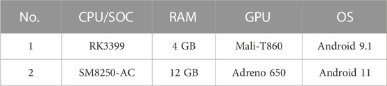
TABLE 2. Testing platform information.
4 Experiment results and discussion
4.1 Dataset refining and expanding
The raw dataset of defects is acquired by the composite plate manufacturer (Zhejiang Jiashan Shuangfei Lubricant Material Co., Ltd.) with an industrial camera installed on the assembly line in production. The dataset contains 960 images with a resolution of 640 × 480 pixels. However, unqualified data, like duplicate images, exist, and a number of different kinds of defect images are unbalanced, which could cause overfitting. Therefore, the datasets need to be arranged to improve the dataset quality.
Defect samples captured by the camera are shown in Figure 9, and they could be classified into two kinds: block and line. Block defects look like black dots, which can happen when external impurities, like small rubber pieces, get burned on the coating surface. Line defects are created by scratching burnt things when the plate is processed by pressure rolls with a line shape.
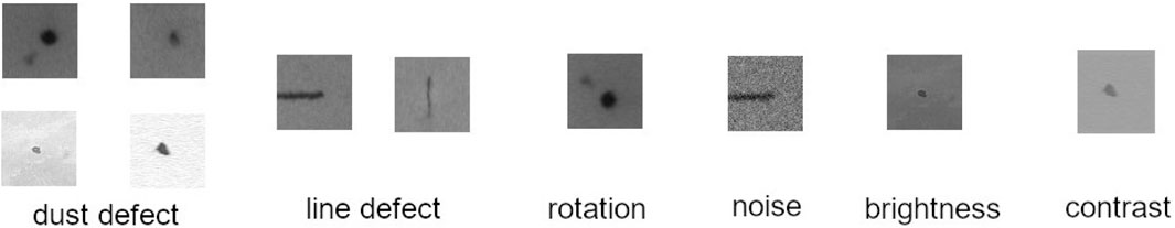
FIGURE 9. Composite plate defect and augmentation samples.
To meet the demand for model training, augmentation is used to create more defect samples from the raw datasets. These defects can be copied and placed with a proper background to generate more available images. All of these images can be polluted by noise, rotated, or adjusted for their contrast and brightness to create more usable counterpart images. Meanwhile, original defects can be modeled afterward to generate pseudo-defects and placed randomly to extend datasets. Augmentation samples are shown in Figure 9.
When enough images are created, the ground truth of images needs to be marked and prepared for model training. The YOLOv5 series use text file (.txt) to mark the ground truth for every separated image file, but the common toolkit LabelImg came out with xml format, which is incompatible [38]. Thus, the xml2txt toolkit is used for transforming an xml file to a text file. After labeling, the datasets are prepared with images and corresponding ground-truth marking files.
After augmentation, each category is defect-free, and the block defect and line defect contain 500 images. The images were divided into three groups: the training group with 1,050 images, the validation group with 150 images, and the testing group with 300 images.
4.2 Model performance comparison
The CPDD-CLMM was compared with other lightweight models, like YOLOv5n, YOLOv5-Lite, and YOLOv7-tiny. Test datasets were divided into three groups: training, detecting, and evaluating. Precision, recall, and accuracy are defined as follows:
In Eqs. 1, 2, TP is true positive, defined as detected objects with an IoU above 0.5. FP is false positive and represents detected objects with an IoU below 0.5. FN is false negative, as objects were not detected.
The PR curve contained interpolated precision for 11 recalls at the 0–1 level. Pinterp is the maximum precision collection of 11 recalls. mAP, the mean AP, is the average of all classes’ APs.
The F1-score, called the balanced F-score, is defined as the harmonic mean of the precision and recall, as Eq. (4)shows, which can be a measure of model accuracy. Meanwhile, the receiver operating characteristic—area under the curve (ROC-AUC) can be also used to measure the ability of the model for classification.
To simulate a regular working environment, all of these platforms run in their normal processor power status, without the limit of the built-in dynamic acceleration function. Defect-detection examples are shown in Figure 9, and the comparison of model characteristics is shown in Table 3. As Chen et al. [20] tested many other lightweight models (YOLOv3-tiny, YOLOv4-tiny, and NanoDet) and YOLOv5-Lite obtained the best result in speed and precision, we chose it as the contract and omitted redundant experiments.
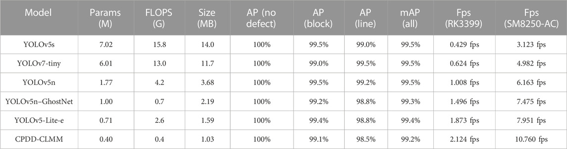
TABLE 3. Model characteristic and test result comparison.
Table 3 shows that CPDD-CLMM has a size of 28.0% and 9.5% FLOPS cost compared with baseline YOLOv5n, and even less for YOLOv5s. In this aspect, the modified model became the best. However, the decrease in model scale could seriously decrease precision. Inference precision was tested and shown in Table 3 as well.
Figure 12A shows the model training parameters results, and Figure 12B shows the F1, P, PR, and R curves of the defects. Figure 12A shows that the loss decreases and precision increases till the 727 epochs. Box_loss, obj_loss, and cls_loss correspond to bounding box loss (loss of bounding box size and position), object loss (loss of numbers of defects), and class loss (loss of defect class identification), respectively. Precision, recall, and mAP curves are also displayed. The maximum limit of the training epoch is 2,000 to train the model as fully as possible. An early stopping method is used to stop the training procedure when the loss of the model stops increasing in the preset epoch limit, and we set the early stopping epoch limit to 100. The best mAP will be recorded in the training procedure, and when the mAP no longer increases for 100 epochs, the early stopping will be trigged. In this case, it was trigged at 727 epochs. Then, the weights corresponding to the best mAP record were saved as the result. In addition, the cause of loss and precision peak, as shown in Figure 12A, could be incidental as the local maximum of loss function as the peak only shows one time. It may be solved when the datasets are extended with more available images.
Figure 12B shows the precision result of the model. The F1-score shown in the F1 curve chart is 0.96 for all classes, and 0.988 mAP is shown in the PR curve chart, which means that the model could identify the defects and distinguish their kinds properly. The model reached 99.1% precision on block defect detection, with only a 0.4% difference from the original YOLOv5 series. The precision decreased by 0.7% for line defects. The precision decreased by 0.3% on average. Generally, the model precision loss is acceptable and still qualified for industrial defect detection as its mAP is 0.988.
4.3 Optimization analysis
To optimize the backbone, we use the GR-Stem block and AGR-Downsample block with specialized simplification and combine GhostConv and the C3-Ghost module to simplify the model neck. By using the simplified blocks, the model is significantly lightweight, as shown in Table 3.
Furthermore, a CBAM is inserted into the model to enhance detection performance. To analyze its effectiveness, the visualization toolkit is used to draw the attention diagram. Kazaj created a YOLOv5 Grad-CAM Python program based on Grad-CAM++ and shared it on GitHub. Grad-CAM++ uses a weighted combination of the positive partial derivatives of the last convolutional layer feature maps with respect to a specific class score as weights to generate a visual explanation for the class label under consideration. As shown in Eq. (4),
The program was modified and used for studies on attention module effectiveness. First, the source code of modules used in models was added to the common .py file. Then, the program parameter is changed according to the model structure. Last, the program is run with a trained model file and target image, and the output image with a gradient map will be generated in the same directory of the target.
Figure 10 shows the defects and corresponding attention gradient map. Samples a2 and b2 revealed that the attention module focused on the main part of the defects, like the line defect body in b2. The attention module in this model did add more attention to the defects. Moreover, a test was made by removing the CBAM and regenerating the model to observe how it affects the model performance.
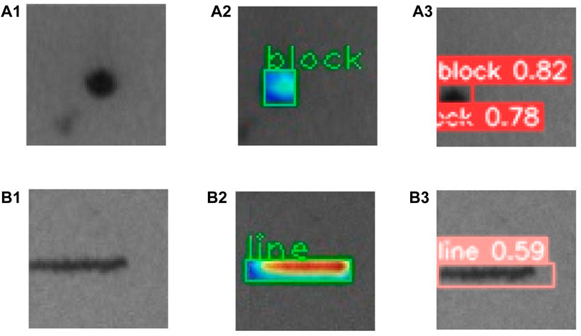
FIGURE 10. Defect attention gradient and detection examples. (A1,B1) are origin defects, (A2,B2) are detection gradient maps and (A3,B3) are detection results.
For comparing the effectiveness of transfer learning, we trained the model with the target dataset 50 times as standard. Then, we trained the model with the LED defect dataset 10 times and chose the best precision weight result as the pre-weight. Then, the model was trained with the generated pre-weight 50 times. Figure 11 shows the epochs obtained by direct training, and transfer learning training used LED datasets. Furthermore, it can be seen that the transfer learning makes the training procedure quicker than direct training, as transfer learning takes fewer epochs to finish the training procedure.
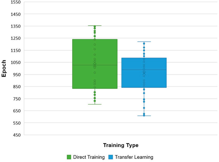
FIGURE 11. Training finishing epoch statistics.
After being converted to PyTorch Mobile .ptl format, the model precision is decreased. The standard of confidence is defined as 0.3 instead of 0.5. A working screenshot is shown in Figure 9. Each image was processed 10 times for inference, with nine randomly chosen images. The definition of TP remained unchanged because the changing of the platform only affects the inference speed and confidence.
The attention module enabled the model to focus more on defects and increased the mAP of line defects to 96.8%. The transfer learning method even improved it to 98.5%. The module and method used by the model increased the precision significantly, as shown in the data given in Table 3.
Table 3 shows that the modified network is faster than the baseline YOLOv5 series, as its frame rate of 2.124 fps is almost double the speed of the original YOLOv5, 1.008 fps, on the RK3399 platform. Meanwhile, a better processor significantly increased the inference speed, as a frame rate of 8.522 fps on the SM8250-AC (1xA77 at 3.2GHz, 3xA77 at 2.4GHz, and 4xA55 at 1.8 GHz) platform is four times faster than 2.007 fps on RK3399 (2xA72 at 1.8GHz and 4xA53 at 1.5 GHz). Speed differences of the models are not the same on platforms 1 and 2, which can be explained by the platforms’ multi-core and multi-thread arrangement and efficiency difference.
4.4 Summary
As described previously, we refined and expanded the raw dataset of defects acquired by the manufacturer and acquired the LED defect dataset for transfer learning. Then, the model we designed with structure simplification and attention enhancement was trained by a transfer learning method and validated with a composite plate defects dataset to test its precision performance. Last, the model was deployed on the RK3399 ARM64 platform to test its speed performance.
In these stages, contrast tests were progressed to prove the effectiveness of our work. Direct training and transfer learning were compared, which showed that the transfer learning does make the training procedure faster with fewer epochs, as shown in Figure 11. Our lightweight model converged with the training procedure in the loss and precision curves shown in Figure 12A and achieved fewer params and smaller size with considerable precision, as shown in the F1 and PR curves given in Figure 12B and Table 3. Meanwhile, more lightweight models, like YOLOv5-Lite-e, are tested on the platform, along with our model, to demonstrate our model speed, as shown in Table 3.
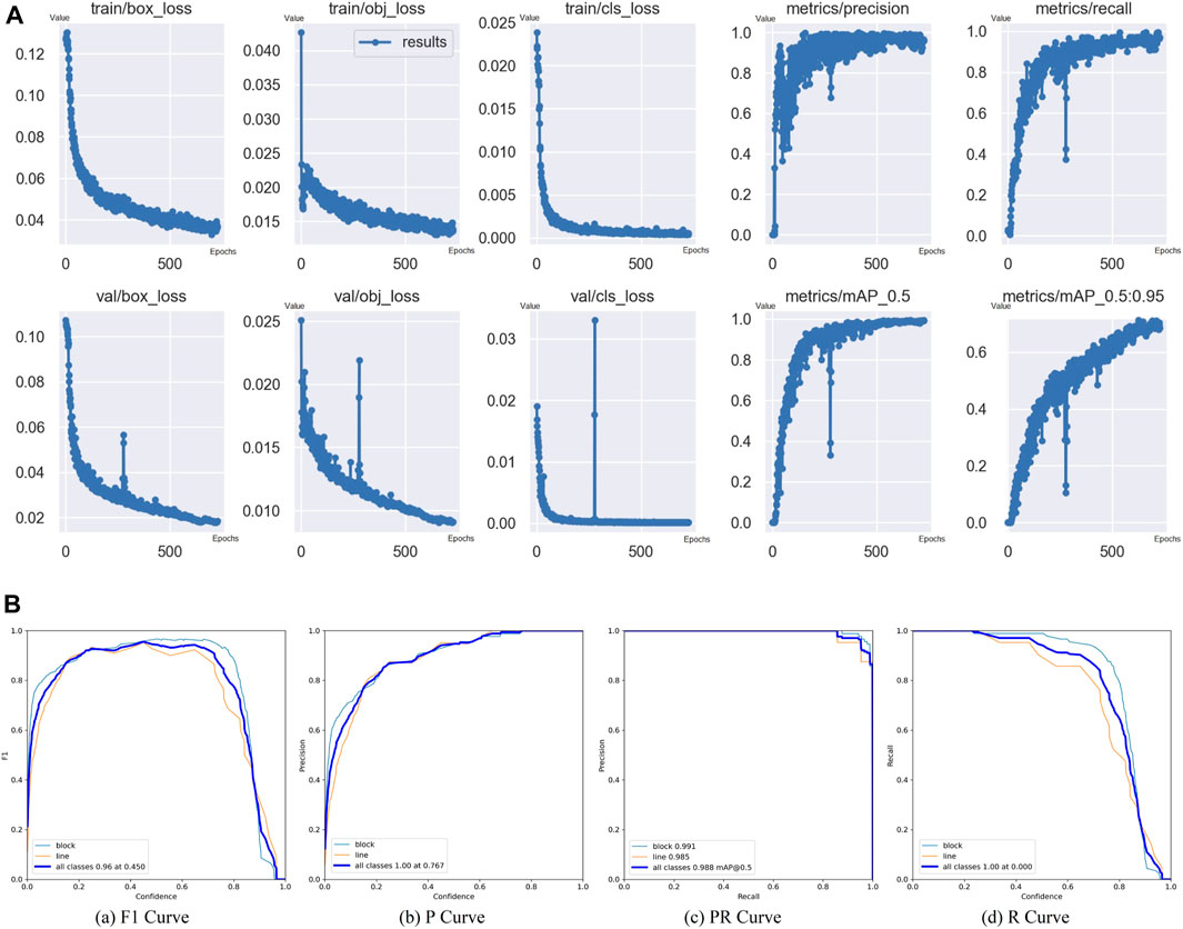
FIGURE 12. (A) Model training parameters results and (B) evaluation results(with transfer training pre-weight, 727 epochs in total). Evaluation metric curves include block and line defects’ information. For PR curve, it contains defect detection results without defect-free results, so the mAP is 99.2% not 98.8%.
Based on these results, we concluded that the model is lightweight and precise enough to achieve real-time defect detection on the ARM64 platform.
5 Conclusion and discussion
The existing production line needs a small and effective solution for its additional function attachment, with less space remaining after long-term modification. The ARM64 mobile platform is a good choice with its small size, extensibility, and stability. To enable a deep learning defect-detection model running on the mobile platform, proper simplification and compensation should be made to make it lightweight and precise enough. The CPDD-CLMM was put forward in the current study for composite plate defect detection on the mobile platform by reducing the redundancy of similar feature maps. The model contains a simplified backbone consisting of GR-Stem and AGR-Downsample modules to improve inference speed, and the CBAM was inserted in the proper position to compensate for decreased precision. The neck and head parts of the model are also simplified with C3-Ghost and GhostConv modules. A transfer training method is also used to improve its precision and training speed. The model can be translated to the PyTorch Mobile format and deployed on Android ARM64 platforms without the specified manufacturer’s hardware dependency, making it suitable for industry deployment.
From the testing data collected, the CPDD-CLMM achieved increased speed and precision maintenance on ARM64 platforms. The model had an inference speed of 2.124 fps on the RK3399 platform and 10.760 fps on the SM8265-AC platform, which was 210.7% and 174.6% more than the speed of the original YOLOv5n and other networks, with only a 0.3% decrease in the mAP at 99.2%. The current study combined advantages from different kinds of object-detection network design, specialized in speed optimization, and produced a practical lightweight solution on ARM64 mobile platforms.
Although such progress has been made, some improvements could be made in the future. First, the defect dataset could be enriched further to improve the defect-detection performance, as the dataset we obtained only contains a limited number of images. Second, an increasing number of new ARM64 processors possess a neural network processing unit (NPU), like Rockchip RK3588 and Qualcomm Snapdragon 8 Gen3, and we can use the NPU to accelerate the model inference further. Third, in this article, we assumed that the defect-detection task of LED is highly relative to the task of composite plates, and the transfer learning method is applied based on that. More defect datasets could be used for a transfer learning test and to find out the relationship between dataset properties and transfer learning effects.
Apart from the aforementioned limitations, how to directly train and run the network on the ARM64 platform could be worked on as the improvement in the ARM64 platform’s hardware and software support. The defect-detection system would be smarter if the network could retrain and update itself locally. We would continue our cooperation with the manufacturer to perfect the dataset and try to deploy the system on the production line eventually.
Data availability statement
The raw data supporting the conclusion of this article will be available on request from the corresponding author BH upon reasonable request.
Author contributions
BW: funding acquisition, supervision, writing–original draft, and conceptualization. YH: data curation, methodology, software, visualization, and writing – original draft. YY: resources, writing–review and editing, and formal analysis. YW: supervision, validation, and writing–review and editing. HL: formal analysis, investigation, and writing–review and editing. BH: funding acquisition, resources, writing–review and editing, and project administration. JC: resources and writing-original draft.
Funding
The authors declare financial support was received for the research, authorship, and/or publication of this article. This study was funded by the Hefei Municipal Natural Science Foundation (2022022) and National Natural Science Foundation of China (51975178).
Conflict of interest
Author JC was employed by Zhejiang Jiashan Shuangfei Lubricant Material Co., Ltd.
The remaining authors declare that the research was conducted in the absence of any commercial or financial relationships that could be construed as a potential conflict of interest.
Publisher’s note
All claims expressed in this article are solely those of the authors and do not necessarily represent those of their affiliated organizations, or those of the publisher, the editors, and the reviewers. Any product that may be evaluated in this article, or claim that may be made by its manufacturer, is not guaranteed or endorsed by the publisher.
References
1. Mordia R, Kumar Verma A. Visual techniques for defects detection in steel products: a comparative study. Eng Fail Anal (2022) 134:106047. doi:10.1016/j.engfailanal.2022.106047
2. Wang B, Zhou Y, Wang Y. Application of improved faster r-cnn network in bubbles defect detection of electronic component led. J Electric Meas Instrumentation (2021) 35:136–43. doi:10.13382/j.jemi.B2003691
3. Wang Z, Jin L, Wang S, Xu H. Apple stem/calyx real-time recognition using yolo-v5 algorithm for fruit automatic loading system. Postharvest Biol Tech (2022) 185:111808. doi:10.1016/j.postharvbio.2021.111808
4. Viola P, Jones M. Rapid object detection using a boosted cascade of simple features. In: Proceedings of the 2001 IEEE Computer Society Conference on Computer Vision and Pattern Recognition. CVPR 2001, 1 (2001). doi:10.1109/CVPR.2001.990517
5. Dalal N, Triggs B. Histograms of oriented gradients for human detection. In: 2005 IEEE Computer Society Conference on Computer Vision and Pattern Recognition (CVPR’05), 1 (2005). p. 886–93. doi:10.1109/CVPR.2005.177
6. Bui M-T, Frémont V, Boukerroui D, Letort P. Deformable parts model for people detection in heavy machines applications. In: 2014 13th International Conference on Control Automation Robotics and Vision (ICARCV) (2014). p. 389–94. doi:10.1109/ICARCV.2014.7064337
7. Girshick R, Donahue J, Darrell T, Malik J. Rich feature hierarchies for accurate object detection and semantic segmentation. In: 2014 IEEE Conference on Computer Vision and Pattern Recognition (2014). p. 580–7. doi:10.1109/CVPR.2014.81
8. Girshick R. Fast r-cnn. In: 2015 IEEE International Conference on Computer Vision (ICCV) (2015). p. 1440–8. doi:10.1109/ICCV.2015.169
9. He K, Zhang X, Ren S, Sun J. Spatial pyramid pooling in deep convolutional networks for visual recognition. IEEE Trans Pattern Anal Machine Intelligence (2015) 37:1904–16. doi:10.1109/TPAMI.2015.2389824
10. Ren S, He K, Girshick R, Sun J (2016). Faster r-cnn: towards real-time object detection with region proposal networks. arXiv e-prints. doi:10.48550/arXiv.1506.01497
11. Pham M-T, Courtrai L, Friguet C, Lefevre S, Baussard A. Yolo-fine: one-stage detector of small objects under various backgrounds in remote sensing images. Remote Sensing (2020) 12:2501. doi:10.3390/rs12152501
12. Redmon J, Divvala S, Girshick R, Farhadi A. You only look once: unified, real-time object detection. In: 2016 IEEE Conference on Computer Vision and Pattern Recognition (CVPR) (2016). p. 779–88. doi:10.1109/CVPR.2016.91
13. Redmon J, Farhadi A. Yolo9000: better, faster, stronger. In: 2017 IEEE Conference on Computer Vision and Pattern Recognition (CVPR) (2017). p. 6517–25. doi:10.1109/CVPR.2017.690
14. Redmon J, Farhadi A. Yolov3: an incremental improvement (2018). arXiv e-prints. doi:10.48550/arXiv.1804.02767
15. Yi Z, Yongliang S, Jun Z. An improved tiny-yolov3 pedestrian detection algorithm. Optik (2019) 183:17–23. doi:10.1016/j.ijleo.2019.02.038
16. Bochkovskiy A, Wang C, Liao H. Yolov4: optimal speed and accuracy of object detection (2020). arXiv e-prints. doi:10.48550/arXiv.2004.10934
17. Jocher G. Ultralytics yolov5 in pytorch (2022). Available at: https://github.com/ultralytics/yolov5.
18. Howard A, Zhu M, Chen B, Kalenichenko D, Wang W, Weyand T, et al. Mobilenets: efficient convolutional neural networks for mobile vision applications (2017). arXiv e-prints. doi:10.48550/arXiv.1704.04861
19. Sandler M, Howard A, Zhu M, Zhmoginov A, Chen L. Mobilenetv2: inverted residuals and linear bottlenecks. In: 2018 IEEE/CVF Conference on Computer Vision and Pattern Recognition (2018). p. 4510–20. doi:10.1109/CVPR.2018.00474
20. Chen J, Zhang D, Suzauddola M, Zeb A. Identifying crop diseases using attention embedded mobilenet-v2 model. Appl Soft Comput (2021) 113:107901. doi:10.1016/j.asoc.2021.107901
21. Zhang X, Zhou X, Lin M, Sun J. Shufflenet: an extremely efficient convolutional neural network for mobile devices. In: 2018 IEEE/CVF Conference on Computer Vision and Pattern Recognition (2018). 6848–56. doi:10.48550/arXiv.1707.01083
22. Ma N, Zhang X, Zheng H-T, Sun J. Shufflenet v2: practical guidelines for efficient cnn architecture design. In: Computer vision – eccv 2018 (2018). p. 122–38. doi:10.1007/978-3-030-01264-9_8
23. Huang M-L, Lin T-Y. Considering breast density for the classification of benign and malignant mammograms. Biomed Signal Process Control (2021) 67:102564. doi:10.1016/j.bspc.2021.102564
24. Chen Z, Yang J, Chen L, Jiao H. Garbage classification system based on improved shufflenet v2. Resour Conservation Recycling (2022) 178:106090. doi:10.1016/j.resconrec.2021.106090
25. Wang XL, Robert J, Ling CX. Pelee: a real-time object detection system on mobile devices. 32nd Conference on Neural Information Processing Systems, Montreal, Canada NeurIPS (2018). doi:10.48550/arXiv.1804.06882
26. Piao Z, Zhao B, Tang L, Tang W, Zhou S, Jing D. Vdetor: an effective and efficient neural network for vehicle detection in aerial image. In: 2019 IEEE International Conference on Signal, Information and Data Processing (ICSIDP) (2019). 1–4. doi:10.1109/ICSIDP47821.2019.9173158
27. Han K, Wang Y, Tian Q, Guo J, Xu C, Xu C. Ghostnet: more features from cheap operations. In: 2020 IEEE/CVF Conference on Computer Vision and Pattern Recognition (2020). (CVPR). 1577–1586. doi:10.1109/CVPR42600.2020.00165
28. Zhong Z, Lin Z, Bidart R, Hu X, Wong A. Squeeze-and-attention networks for semantic segmentation. In: 2020 IEEE/CVF Conference on Computer Vision and Pattern Recognition (CVPR) (2020). 13062–71. doi:10.1109/CVPR42600.2020.01308
29. Deng J, Ma Y, ao Li D, Zhao J, Liu Y, Zhang H. Classification of breast density categories based on se-attention neural networks. Comp Methods Programs Biomed (2020) 193:105489. doi:10.1016/j.cmpb.2020.105489
30. Park J, Woo S, Lee JY, Kweon IS. Bam: bottleneck attention module. In: Computer vision – eccv 2018 (2018). doi:10.48550/arXiv.1807.06514
31. Woo S, Park J, Lee J, Kweon I. Cbam: convolutional block attention module. In: Computer vision – eccv (2018). p. 3–19. doi:10.1007/978-3-030-01234-2_1
32. Liang T, Lv B, Zhang N, Yuan J, Zhang Y, Gao X. Prohibited items detection in x-ray images based on attention mechanism. J Phys Conf Ser (2021) 1986:012087. doi:10.1088/1742-6596/1986/1/012087
33. Liao Q, Wang D, Xu M. Category attention transfer for efficient fine-grained visual categorization. Pattern Recognition Lett (2022) 153:10–5. doi:10.1016/j.patrec.2021.11.015
34. Yang L, Yan J, Li H, Cao X, Ge B, Qi Z, et al. Real-time classification of invasive plant seeds based on improved yolov5 with attention mechanism. Diversity (2022) 14:254. doi:10.3390/d14040254
35. Jamil F, Verstraeten T, Nowé A, Peeters C, Helsen J. A deep boosted transfer learning method for wind turbine gearbox fault detection. Renew Energ (2022) 197:331–41. doi:10.1016/j.renene.2022.07.117
36. Zitong Wang MH, Yang R, Zeng N, Liu X. A review on transfer learning in eeg signal analysis. Neurocomputing (2021) 421:1–14. doi:10.1016/j.neucom.2020.09.017
37. Chander S. Java se 17 and jdk 17 api documentation system currenttimemills and nanotime (2021). https://docs.oracle.com/en/java/javase/17/docs/api/java.base/java/lang/System.html.
38. Lin T. Labelimg python package index page (2021). Available at: https://pypi.org/project/labelImg/.
39. Chattopadhay A, Sarkar A, Howlader P, Balasubramanian VN. Grad-cam++: generalized gradient-based visual explanations for deep convolutional networks. In: 2018 IEEE Winter Conference on Applications of Computer Vision, Lake Tahoe, NV, United States. WACV (2018). 839–47. doi:10.1109/WACV.2018.00097
40. Chen X, Gong Z. Yolov5-lite: lighter, faster and easier to deploy (2021). doi:10.5281/zenodo.5241425
41. Pytorch open source project. Pytorch mobile for android mobile devices (2022). Available at: https://pytorch.org/mobile/android/.
42. Pytorch open source project. Pytorch mobile object detection demo github page (2022). Available at: https://github.com/pytorch/android-demo-app/tree/master/ObjectDetection.
Keywords: composite plate, defect detection, You Only Look Once, embedded optimization, PyTorch Mobile
Citation: Wang B, Huang Y, Yang Y, Wang Y, Li H, Huang B and Chen J (2023) CPDD-CLMM: a comprehensive lightweight mobile-optimized network for composite plate defect detection. Front. Phys. 11:1264636. doi: 10.3389/fphy.2023.1264636
Received: 21 July 2023; Accepted: 01 November 2023;
Published: 20 November 2023.
Edited by:
Sushank Chaudhary, Chulalongkorn University, ThailandReviewed by:
Amir Parnianifard, University of Electronic Science and Technology of China, ChinaAbhishek Sharma, Guru Nanak Dev University, India
Copyright © 2023 Wang, Huang, Yang, Wang, Li, Huang and Chen. This is an open-access article distributed under the terms of the Creative Commons Attribution License (CC BY). The use, distribution or reproduction in other forums is permitted, provided the original author(s) and the copyright owner(s) are credited and that the original publication in this journal is cited, in accordance with accepted academic practice. No use, distribution or reproduction is permitted which does not comply with these terms.
*Correspondence: Bin Huang, hbld@hfut.edu.cn