 Shinichi Saito
- Center for Exploratory Research Laboratory, Research & Development Group, Hitachi, Ltd., Tokyo, Japan
Orbital Angular Momentum (OAM) of photons are ubiquitously used for numerous applications. However, there is a fundamental question whether photonic OAM operators satisfy standard quantum mechanical commutation relationship or not; this also poses a serious concern on the interpretation of an optical vortex as a fundamental quantum degree of freedom. Here, we examined canonical angular momentum operators defined in cylindrical coordinates, and applied them to Laguerre-Gauss (LG) modes in a graded index (GRIN) fibre. We confirmed the validity of commutation relationship for the LG modes and found that ladder operators also work properly with the increment or the decrement in units of the Dirac constant (ℏ). With those operators, we calculated the quantum-mechanical expectation value of the magnitude of angular momentum, which includes contributions from both intrinsic and extrinsic OAM. The obtained results suggest that OAM characterised by the LG modes exhibits a well-defined quantum degree of freedom.
1 Introduction
Quantum commutation relationship between operators is an indispensable characteristic in connection with measurements of physical observables [1–4]. Angular momentum operators are especially important as generators of rotation for states with angular momentum state, |m⟩, which is characterised with a quantised integer or a half-integer, m, along a certain direction (say, z) [1–4]. The states pointing directions such as x- and y-directions or any other directions in three-dimensional (3D) space are described by superposition states of orthogonal basis states [1–4], and commutation relationship is used to rotate the states. The spin,
However, this elegant theoretical framework of angular momentum is less trivial in applying to a photon [5–13], since a photon is usually uni-directionally propagating (say, along z). Therefore, the apparent spherical rotational symmetry is absent for a photon, such that the situation is rather different from that of an electron confined in a spherically symmetric 3D space. The propagation direction of a photon sets a natural quantisation axis; along the propagation direction, the angular momentum operator,
The nature of structured light is attracting significant attention, these days [18–23]. The increased bandwidth in fibre optic communication would be one of the most promising near-term application [20, 24]. Another attractive application will be for quantum technologies, where classical entanglement with orthogonal spin and orbital angular momentum states are correlated over variable space and time [18–23, 25–30].
Nevertheless, there are several naive questions, which should be addressed: 1) The spin of a photon could be proper angular momentum, which would satisfy commutation relationship, at least in the absence of OAM. The selection rules of absorption and excitation of a photon in materials [2–4, 9, 31] are clear evidence to expect that the spin of a photon is transferred to angular momenta of an electron. If the spin of a photon is conserved, while accepting well-defined OAM of an electron, why is it regarded as a classical degree of freedom, which is described by a commutable operator? It should be treated with an appropriate quantum commutation relationship, if spin of a photon is a proper quantum mechanical degree of freedom. Moreover, what about the relationship between spin of a photon and the polarisation [32, 33]? Detailed discussion about spin of photons will be provided in a separate paper [28]. 2) A photon with OAM carries quantised angular momentum of ℏm along the direction of propagation, which was successfully described by a Laguerre-Gauss (LG) mode in cylindrical coordinates [5]. Here, some questions arise: Why ℏ appeared in OAM, which is usually the evidence of quantisation? If the OAM is a classical degree of freedom, described by a commutable operator, we normally expect that ℏ would not appear, which is clearly not the case. Can we define standard quantum mechanical canonical angular momentum operators and apply them to LG modes? Moreover, what happens if we define ladder operators for raising or lowering angular momentum in a standard way, such as
Here is the outline of this paper: In Section 2, we derive fundamental principles and equations, which we are relying on, and explain our model. We are interested in photonics that can be applied to communication technologies and low-energy condensed-matter physics. Consequently, we will not deal with high-energy physics nor those issues related to Lorentz invariance [7, 8, 15, 16] in this paper. We are considering monochromatic coherent light from lasers, such that the incoherent unpolarised light will not be considered, either. The incoherent unpolarised light corresponds to a beam that the radius of the Stokes parameters (S1, S2, S3) does not coincide with its intensity,
In Section 3, we explain our methods to evaluate OAM operators. We clarify the challenges to apply OAM operators to plane-waves, which are not successful. Nevertheless, this would help to understand the problem, which we would like to address. There, we show that the main problem of the plane-waves is a lack of a node at the core of the waveguide, which is also called as topological charge. We show that this problem is solved by using LG modes. In Section 4, we show our main calculation results of various matrix elements for OAM and discuss their implications. Our results show that the LG modes actually satisfy the quantum canonical commutation relationship of angular momentum. We also obtained expectation values of the magnitude of OAM. Finally, in Section 5, we conclude that OAM is indeed a genuine quantum-mechanical observable at least in a graded index (GRIN) fibre [9, 34] satisfying some conditions.
2 Principles and models
2.1 Maxwell’s equations
We start from Maxwell’s equations [9, 10],
in a non-magnetic transparent material of the dielectric constant ϵ and the permittivity μ0 without charges and currents. As usual for describing electromagnetic fields [9, 10], we use complex oscillation fields in SI units for electric field
which is valid in a completely uniform material and in vacuum. In this paper, we will examine the Helmholtz equation in more detail as follows, but we will not examine its validity any further. The only source of deviations would be arising from the case with significant non-uniformity (∇ϵ ≃ 0). Therefore our analysis will not be valid if ϵ is significantly changed in nano-metre-scale such as for photonic crystals [35–38] and other inhomogeneous systems [39, 40].
2.2 Mapping to Schrödinger equation
First, we see the qualitative feature of the Helmholtz equation in a uniform material by assuming a solution for a linearly polarised monochromatic plane wave
where E0 is the magnitude of the electric field, k is the wavenumber in the material, ω is the angular frequency, the unit vector
For various practical applications in laser optics, rays from laser sources are sufficiently collimated, such that the rays can be regarded as paraxial beams [9]. In such a case, we can use slowly varying approximation [9] to neglect the second derivative,
and obtain [41]
where we have used the dispersion relationship, ω = vk, with the velocity
for a particle of mass, m, in a 2D xy-plane at time t. The correspondence is summarised in Table 1.
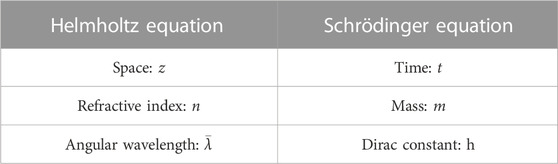
TABLE 1. Mapping of Helmholtz equation to a non-relativistic Schrödinger equation.
This implies the propagation of a photon along a paraxial optical path follows the same equation, which describes the dynamics of a massive quantum-mechanical particle [41]. In fact, electron vortices similar to photonic ones were observed [43], and essentially the same mathematical and physical techniques were applicable to both electronic and photonic systems. It is also intuitive to recognise n for a photon corresponds to m of the particle, such that v is low in a material with large n similar to the low velocity of a heavy particle.
2.3 Coherent state for photons
On the contrary to the above similarity between electrons and photons, the important difference is coming from the nature of statistics between Fermions and Bosons. For photons, we are considering monochromatic rays from lasers, which are considered to be in a macroscopic coherent state, exhibiting Bose-Einstein condensation, enabled by the Bose statistics for spin integer particles [1, 4, 11, 44]. On the other hand, electrons are Fermions due to their spin 1/2 characteristics [1, 4], such that a macroscopic coherence is not expected, except for ordered states, such as a superconducting state, which is similar to Bose-Einstein condensation of Cooper pairs [45]. Here, we consider a coherent state for photons to understand the quantum-mechanical state with certain polarisation and orbital angular momentum. A coherent state cannot be described by a fixed number state only due to the phase coherence. Instead, a coherent state is described by a fixed phase, while allowing fluctuation in the number of photons from their average value by a superposition of states with different number of states [11, 44]. Specifically, a coherent state for σ-polarisation in a uniform material is described by
where σ = H for horizontally polarised state and σ = V for vertically polarised state. ασ is a complex number, accounting for the macroscopic wavefunction [28]. We use horizontally or vertically polarised states as basis states, for simplicity, but in general we can take other orthonormal bases such as left/right polarised states and diagonal/anti-diagonal states [9].
where δ is the Kronecker delta. A coherent state is best characterised by the fact that it is an eigenstate of an annihilation operator, which can be directly confirmed by the commutation relationship as
We can also confirm that |ασ⟩ is normalised as ⟨ασ|ασ⟩ = 1. Then, we can calculate the average number of photons for both polarised states as
where NH and NV are the average number of photons for horizontally and vertically polarisation, respectively, N = NH + NV is the total number of photons, and α is the auxiliary angle
where δ ∈ (0, 2π) is the phase of the polarisation. The overall coherent state is described by the direct product as
Now, we have prepared the coherent state, and the next step is to consider the quantum many-body description of the electromagnetic field, which is achieved by considering the following complex electric field operator
where V is the volume,
we realise the state is an eigenstate of
where
where the matrix part is nothing but a Jones vector [9] to describe the polarisation state of a photon. Moreover, the overall factor of the complex electric field of E0eiβ corresponds to the orbital part of the wavefunction for photons in a uniform material, which is the solution of Helmholtz equation.
More generally, for describing a coherent monochromatic ray from a laser source propagating in a waveguide or a fibre, the complex electric field operator must be defined as
where the scalar complex electric field,
where the orbital part is described by Ψ(r) = ψ(r)eiβ. Ψ(r) is determined by the scalar Helmholtz equation
and thus Ψ(r) is essentially a single-particle wavefunction, describing the orbital degree of freedom. The reason why a macroscopic number of photonic state can be described by a single wavefunction comes from the Bose-Einstein condensed character of a superposition state. All photons are occupying a single state with fixed ω, k, δ, and α, while allowing the fluctuation of the number of photons around its average value of N using a coherent state. The polarisation state is also described as a superposition state of two orthogonal polarisation basis states, coming from intrinsic internal degrees of freedom described by a Jones vector.
The coherent state for a laser beam can also be written as
If we want to calculate the real electric field, instead of the complex field, we should use the electric field operator defined by
which is an observable, such that we can calculate the expectation value,
2.4 Laguerre-Gauss mode in a uniform material
Above formalism is based on Maxwell equations, quantum statistics, and superposition principle. Therefore, it is virtually an exact consequence that Ψ(r) represents the wavefunction of coherent photonic states and satisfies the Helmholtz equation at least in a uniform material. The similarity of quantum-mechanical nature of Ψ(r) was intuitively suggested in many pioneering works [5, 6, 8, 14]. Now, it becomes clearer that the intuitive correlation is not merely a coincidence but firmly supported by a quantum many-body theory rather than classical Maxwell’s equations alone, since we cannot derive a wavefunction from classical mechanics. Our formalism contains a standard vacuum state of Quantum Electro-Dynamics (QED) theory [4] in the limit of n → 1, where Ψ(r) will become a simple plane wave, Ψ(r) → eiβ.
However, the plane wave is not the only solution of the Helmholtz equation, since a solution of differential equation depends also on the symmetry and boundary condition of the system [5, 9]. This is especially true in condensed matter physics, because a material is usually patterned in a specific form with a certain symmetry. Here, we derive a LG mode solution in a uniform material in cylindrical coordinates by using the slowly varying approximation [5, 9]. For completeness, we will describe its full detail in this subsection.
Our starting point is the Helmholtz equation in cylindrical coordinates (r, ϕ)
where
where w(z) is the beam-waist size, P(z) is the phase shift for a beam expansion, q(z) is the complex spherical radius, and θ(z) is another phase shift for radial and azimuthal expansions. Here, we tentatively assume m ≥ 0 for simplicity, and yet we relax this condition for all integer values, including negative values, at the end of the calculation. While the trial wavefunction is inserted into the Helmholtz equation, it is useful to note that ∂x (fg) = g (∂xf ) + f (∂x g) = ψ(∂x f )/f + ψ∂x g/g holds. Then, we obtain
The Gaussian mode solution is given by assuming
which will give us q(z) = z + q0 = z − iz0 and
and the phase-shift factor
where the beam waist, w(z), the beam radius, R(z), and the phase, η(z), are given by
The focal point of the Gaussian beam is set at the origin, where the waist becomes minimum w (0) = w0. In a uniform material or a vacuum, there is no mechanism to confine the mode, and the beam waist can be arbitrarily controlled by the use of an optical lens up to the diffraction limit. Thus, w0, and consequently z0, can be controlled and determined by a boundary condition. It is also useful to note that kww′ = 2z/z0 and
We now focus on the last three terms of this equation, which can be rewritten by exchanging valuables subsequently using ρ = r/w, a = ρ2, and b = 2a as
where we used the differential equation for the associate Laguerre function,
such that we can obtain
which gives the phase-shift
Finally, we obtain
which is not normalised, yet. The norm Nnorm of the wavefunction is obtained by
where we used the orthogonality condition (Section 4)
Thus, we obtain
Now, we consider the case for a negative value of m. The only source of the azimuthal dependence in the Helmholtz equation is coming from
such that the solution does not depend on the sign of m.
Therefore, the final normalised wavefunction becomes
Here, the wavefunction was normalised in the xy-plane as
since our main interests in the following sections are orbital angular momentum, and this normalisation is easier to treat. On the other hand, in the consideration of the electric field in the previous subsection, the normalisation was slightly different, since we have prioritised to have the proper definition of E0 (V/cm) as the electric field. When the number of photons that we are considering is one, this corresponds to the zero-point fluctuation of the electric field,
It is worth making a remark on the Gouy phase [5, 42, 46–50] of
which is the same as a geometrical phase of Pancharatnam-Berry. This term appears due to the focusing of the beam, which will change
We should be careful for the interpretation of the radial quantum number, p, which describes the number of nodes along the radial direction. This value is different from the quantum number, l, to describe the magnitude of OAM in a spherical symmetric system by
2.5 Laguerre-Gauss mode in a graded index fibre
As another example, for which the Helmholtz equation can be solved exactly, we also discuss the propagation of a coherent monochromatic laser beam in the GRIN fibre [9, 34], which has the refractive index n(r) dependence given by
With those parameters, we can rewrite
in the cylindrical coordinate, we can convert this equation to
One of the conceptual advantages to consider the GRIN waveguide is that we do not have to worry about the paraxial slowly varying approximation at all, because the second derivative along z vanishes. This can be verified by confirming that the trial wavefunction
with the constant waist w0 and the constant complex radius, q, becomes the solution. Again, we tentatively assume m ≥ 0. By inserting Eq. 53 into Eq. 52, we obtain
we then obtain a stable Gaussian form by noting
we also use useful identities
and the Helmholtz equation then becomes
By noticing that the last three terms in the left-hand side of Eq. 59 can be described by the associated Laguerre function, we obtain
and the remaining equation becomes
This provides the solution [9]
where we have defined a phase velocity at the core as v0 = c/n0 and a frequency shift as δω0 = v0g. By solving Eq. 62 with respect to ω, we obtain the dispersion relationship
This dispersion relationship can be intuitively understood as follows: Since ω ≠ 0 at k = 0, this implies an opening of an energy gap in a band diagram, meaning that the dispersion is “massive.” The emergence of an energy gap is reminiscent of the theory of superconductivity [45] and the Nambu-Anderson-Goldstone-Higgs theory of a broken symmetry [51–54]. We infer that a similar symmetry principle is hidden in our system. We will discuss this in a subsequent paper [55]. Here, we can recognise the increase of the gap by increasing the radial quantum number, p, and the quantised OAM number, m, because the discrete photon energy is related to the confinement degrees of freedom of photons rather than the free propagation of photons along z.
Finally, we relax the condition for m to allow negative integers without breaking the formalism. Normalising the wavefunction as before, we obtain an exact solution
in a GRIN fibre without the slowly varying paraxial approximation.
3 Methods
3.1 Orbital angular momentum for photons
We have confirmed the fundamental principle on how to treat a coherent laser beam on the basis of Maxwell’s equations and a quantum many-body theory. In particular, we have understood why we can describe a macroscopically coherent laser by a single-particle wavefunction, Ψ(r), due to Bose-Einstein statistics, while the entire many-body state is described by a coherent state with both orbital and spin degrees of freedom. Photons are quantum-mechanical particles with a wave nature; we can also describe them with Maxwell’s equations together with a quantum many-body theory. For coherent photons from a laser, it was less obvious how we can treat the ray quantum-mechanically; however, a laser produces indistinguishable photons with the same phase by the stimulated emission process, in which existing photons in a cavity induce recombinations of electron-hole pairs to make clones of photons as a results of a chain-reaction. Thus, we can describe a coherent monochromatic ray by the single mode of Ψ(r). If the waveguide contains several modes, it is straightforward to allow the superposition of these macroscopically coherent beams.
The fundamental equation for describing the orbital character of Ψ(r) is the Helmholtz equation, instead of the Schrödinger equation, although we have a significant similarity to a paraxial wave (Table 1). Unlike in vacuum without a material, where Ψ(r) is a simple plane-wave, the mode profile of Ψ(r) can be highly non-trivial in materials, depending on the symmetries of the waveguides and the actual profile of the refractive index, n(r). In the previous section, we have obtained LG modes in a GRIN fibre with a uniform material. Here, the LG modes (LGnm) were clearly labelled by the radial quantum number n and the quantum optical orbital angular momentum number m along the propagation direction. The central theme of this paper is to examine the validity of this interpretation that m is indeed a proper quantum index to describe the optical OAM, and thus the angular momentum of the orbital is ℏm. Under the assumption that a standard quantum mechanical treatment is also applicable to photons, described by Ψ(r), we examine the impacts of OAM operations in the following sections.
3.2 Canonical orbital angular momentum operators
The most well-established quantum mechanical treatment is canonical commutation relationship for the position
respectively. In a system with a spherical symmetry, the eigenstate of these operators are described by Ylm (θ, ϕ) = ⟨θ, ϕ|l, m⟩, where θ and ϕ are polar and azimuthal angels, respectively, l and m are quantum numbers for the magnitude of OAM and the OAM component along the quantisation axis, respectively [1–3]. Our goal is to obtain a similar relationship for a system with a cylindrical symmetry, described by the LG modes. In this section, we will obtain the operator representation of
The unit vectors of cylindrical coordinates are defined for a rotation in a 3D Cartesian coordinate along the z-axis,
where
and the Laplacian becomes
where we have used
This ϕ dependence of
By inserting these into
We can readily confirm the original commutation relationship
and its cyclic exchanges
are all valid in the cylindrical coordinate (r, ϕ, z).
We also obtain raising and lowering operators, respectively, as
3.3 Application to plane waves and problems
So far, it was straightforward to develop a theory for photonic OAM. In this subsection, we will apply our canonical OAM operator to plane waves to clarify that problems arise. Specifically, we consider a plane wave with OAM in the simplest form:
which is not the solution of the Helmholtz equation at m ≠ 0. Nevertheless, it is useful to clarify the potential issue and to explain what we should address in the following sections.
First, multiplying it by
which means that Ψ is indeed an eigenstate for lz and that
by averaging these over space, we obtain
therefore, the expectation values are reasonably well-defined.
However, if we calculate the complex conjugate of
and multiply this by
which is a positive real value. On the other hand, the direct calculation of
This implies that
which means that the l± is not observable for the Hilbert space spanned by the plane waves with OAM. We can also confirm the conjugate relationships
which also imply
We also see
showing a classical result without providing commutation relationship. This is a remarkable difference from the standard quantum mechanics [3], which shows the canonical commutation relationship upon the calculation of the norm for
On the other hand, the direct calculation shows
such that the commutation relationship
is indeed satisfied on the average.
These apparent contradiction and inconsistency are coming from the assumption of the ill-defined plane-wave wavefunction, Ψ(r, ϕ, z) = eikzeimϕ. This is confirmed by calculating the magnitude of the OAM along the radial direction as
which gives an imaginary part, thus showing that the magnitude is not observable. If we take the average over z ∈ (0, L), we obtain
which is still a complex value. Further average over r ∈ (0, R), where R is the radius of a cylindrical waveguide, gives
which diverges at the origin. We can also integrate over z ∈ (L/2, L/2), and obtain
which becomes a real value, but still diverges at the origin.
The position-dependent average of the radial magnitude suggests that it contains extrinsic contributions of OAM. For both coordinates, we could not avoid the ultraviolet divergences at the origin, which are coming from the finite amplitude of the wavefunction at the origin. Without having a node at the origin, the magnitude of the OAM required to sustain the phase described by eimϕ is impossible to exist.
However, for the LG modes, which always have nodes at the centre (r = 0) of the waveguide for ∀m ≠ 0, there is a chance that the OAM can be well-defined quantum-mechanically. Our main purpose of this work is to confirm the validity of this concept of OAM, using canonical orbital angular momentum operators defined in this section, for the LG modes in a cylindrical GRIN fibre. In the next section, we will confirm positive results, including the observable nature of the magnitude and the commutation relationship for OAM.
4 Mathematical formulas
4.1 Laguerre function
We describe full details of Laguerre and associate Laguerre functions and related formulas in this section [56–58]. First, we consider a differential equation
which will be solved by assuming a Taylor series expansion
which gives
This provides a recurrence formula
for j = 0, 1, 2, …, n, and aj = 0 for j > n. Therefore, we obtain
The differential equation cannot be determined uniquely without providing a boundary condition. The same is true for a special function, such that there exists a room to choose the arbitrary value of a0, while it is a standard rule to choose a0 > 0 in mathematics. Our definition in this paper is a0 = 1, but other people are also using a0 = n! as an alternative definition. In this way, we obtain the solution, f = fn(a), as
where nCj is a binomial coefficient.
4.1.1 Rising operator
By directly calculating the derivative, we obtain
which can be combined with this identity
to obtain
This formula works as a raising operator to increase the radial index, n.
4.1.2 Lowering operator
Quite similarly, we can also obtain the lowering operator. Calculating a derivative,
together with the identity
we obtain the lowering operation formula,
By summing up raising and lowering operators, we also obtain the recurrence relationship
which correlate 3 successive Laguerre functions.
4.1.3 Generating function
The generating function is defined as a function, whose coefficients of series expansion are Laguerre functions. Therefore, it is defined as
By inserting the series expansion form of Li(t), we obtain
where we used k = i − j in the 2nd line. Together with the binomial theorem
we finally obtain the analytic formula for the generating function as
Using this generating function, we can obtain the orthogonality relationship, which is used to confirm the orthogonality against modes with different radial numbers and calculate the normalisation factors. In order to derive it, we evaluate the following sum of the integrals,
Comparing the first term and the last one, we obtain
4.1.4 Rodrigues formula
Rodrigues formula is an operator form of the representation of Laguerre function, which will be suitable for quantum mechanics. In order to obtain it, we just need to evaluate the following function
and thus, we obtain
4.2 Associated Laguerre function
The associated Laguerre function is defined as
The factor of (−1)m guarantees the first Taylor series expansion coefficient of a0 to be positive a0 > 0 as a mathematical convention.
The differential equation for the associated Laguerre function is derived from that of the Laguerre function
by the mth derivative of this equation,
which becomes,
By exchanging n → n + m, we obtain
We also obtain the Taylor series expansion of
which shows that the term at j = 0 is indeed positive.
4.2.1 Generating function
The generating function for the associated Laguerre function is defined by
Using the binomial theorem,
we obtain
4.2.2 Recurrence relationship
We obtain the recurrence relationship for the associated Laguerre function. By calculating the derivative of the generating function by τ, we obtain
Then, we obtain
from which we obtain the recurrence relationship
for n ≥ 1.
4.2.3 Ladder operators for radial quantum number
For obtaining ladder operators, we calculate the derivative of the generating function by t as
which becomes
Then, we obtain the identity for lowering n
However, this expression is not perfect, since the derivative operator remained in the right-hand side, which will be removed later.
Next, we construct the raising operator by calculating the derivative of the recurrence equation by t as
which becomes
by using the lowering identity, this becomes
which gives the raising operator
for n ≥ 1. This expression is preferable, since the derivative operation appeared only in the left-side. Together with this raising operator and the recurrence formula, we can eliminate
while keeping m unchanged. These ladder operations for the associated Laguerre functions are consistent with those for Laguerre function in the limit of m = 0.
4.2.4 Ladder operators for orbital angular momentum
The above formulas for raising and lowering the radial quantum numbers are known in literatures [56–58], while we could not find appropriate formulas for raising and lowering quantum number m for orbital angular momentum without affecting the radial quantum number of n. Here, we derived these by direct calculations. First, we obtain the raising operator by calculating
Thus, the raising operator is described as
It was less straightforward to obtain the lowering operator. As for preparations, we recognised several useful recurrence formulas
By using the recurrence formula, we obtain
Next, we use the raising operator for n to obtain
By combining these equations, we obtain
Inserting this into Eq. (B33), we obtain the lowering operator
4.2.5 Orthogonality relationship
The orthogonality relationship is obtained in a similar way by using the generating function
and calculating the sum
where we used the binomial theorem
Thus, we obtain the orthogonality relationship
4.2.6 Rodrigues formula
The Rodrigues formula for the associated Laguerre function is obtained by the direct calculations. First, we calculate
On the other hand, we calculate
By comparison, we obtain the Rodrigues formula
4.2.7 Integration formulas
We also obtained integration formulas for the associated Laguerre functions:
These are useful to calculate the matrix elements. We also obtained an identity,
5 Results and discussions
We consider applications of the canonical OAM operators to the LG modes in a GRIN fibre. We use the normalised LG mode [5, 6, 8–10]
where n is the radial quantum number and m is the quantum number of OAM along the direction of propagation. In principle, we should also consider a superposition state made of the LG modes with different quantum numbers [59–61], but we will not consider this in this paper for simplicity; yet our formalism works well. We define a normalised cross-sectional area as
5.1 Expectation value
First, we have checked the expectation values of
and thus we obtain
Therefore, the quantum-mechanical expectation value of OAM is well-defined for all directions. This is a single particle expectation value, and the total angular momentum,
5.2 Ladder operations
We will evaluate ladder operations to the LG modes. The calculations are straightforward but tedious, so that we will split them into several sections.
5.2.1 Rising operation for m > 0
We assume m > 0 and calculate
Where the last factor becomes
Where we have used
Therefore, we obtain
The most significant part of this expression is that we confirm
5.2.2 Rising operation for m = 0
We then continue to calculate for m = 0 as
where the last factor becomes
and thus we obtain
which is exactly the same expression with that of m > 0.
5.2.3 Rising operation for m < 0
We obtain a similar result by directly calculating
where the last factor becomes
where we have used
Thus, we obtain
therefore, the raising operator is successfully working to increment m, independently of the value and the sign of m.
5.2.4 Lowering operation for m < 0
Next, we apply the lowering operator to the case for m < 0, and obtain
Where the last factor becomes
Which yields
this also shows that the lowering operator can actually lower m to m − 1.
5.2.5 Lowering operation for m = 0
Similarly, we obtain for m = 0:
Where the last factor becomes
Which yields
This is the same formula as that we obtained for m < 0.
5.2.6 Lowering operation for m > 0
Finally, we apply the lowering operator to the case for m > 0, and obtain
where the last factor becomes
which yields
therefore, the lowering operator is also successfully working to decrement m, independently of the value and the sign of m.
Thus, in this subsection, by obtaining the wavefunction after the ladder operations, we confirmed that the ladder operations work to change the quantised OAM along the propagation direction in units of ℏ.
5.3 Norm after ladder operations
In this subsection, we obtain the norm of the wavefunctions after ladder operations. We calculate it for separately depending on the sign of m, as in the previous subsection. We have extensively used the integration formulas, which are summarised in Section 4.
5.3.1 Norm of
First, we rewire the wavefunction by using the formula,
Then, we obtain
5.3.2 Norm of
Similarly, we obtain
5.3.3 Norm of
Next, we calculate the norm of
5.3.4 Norm of
Finally, we calculate
5.3.5 Summary of the norm of
The above direct calculations show that we obtain the same norm for
which is independent of the sign of m. The first term is coming from the origin dependent extrinsic OAM, while the second term corresponds to the contribution from the intrinsic OAM, which is always positive and finite. The obtained form of
5.4 Validity of commutation relationship for LG modes
First, we must calculate the wavefunction of
5.4.1 Ladder operators
Before calculating the matrix elements, we will describe operators,
and
Thus, we also confirmed the commutation relationship for
therefore, if we apply these operators to an LG mode, we must confirm that this identity is always valid. This is useful to check the validity of the calculation.
5.4.2
First, we evaluate various terms as follows:
and finally
By summing up some of these terms, we obtain
By using the integration formulas (Section 4), we finally obtain
5.4.3
The only source of the difference between
This result, together with the previous result for
where
5.4.4
We can proceed for m ≤ 0 in a similar way. First, we evaluate the factors:
and the other factors are the same ones for m ≥ 0. Then, we obtain
Therefore, we finally obtain
5.4.5
Again, the only source of the change between
Therefore, the commutation relationship over average
is also valid for m ≤ 0.
5.5 Summary of expectation values of
The above results are summarised as follows,
and
which are independent of the sign of m. The commutation relationship over average
is also valid for ∀m.
5.6 Magnitude of OAM
The above calculations have confirmed the quantum commutation relationship,
We can confirm that the expectation value is independent of whether we are using
The expectation value does not depend on the sign of m, which is reasonable in a system with a helical symmetry. The first term contains the origin (z = 0) dependent contribution of the extrinsic OAM. If we take the average over z ∈ (0, L), we obtain
while if we average over z ∈ (−L/2, L/2), it becomes
The other contributions are from intrinsic OAM. If m ≫ 1, the most of the energy of photons is used to sustain the rotating motion as OAM, such that ℏδω0m ≫ ℏv0k in the dispersion relationship. In this limit, the intrinsic OAM is dominated by the contribution from ℏm, which is consistent with the above formula.
In the opposite limit of the absence of the definite quantised OAM (n = m = 0), the beam becomes a simple Gaussian wave. Even in this case,
holds, which is an intuitive formula, because the same amount of the angular momentum magnitude with spin of ℏ is subtracted. The finite intrinsic OAM is coming from quantum mechanical fluctuations due to
where
5.7 Transfer matrix element
Finally, we calculate the matrix elements of
for m ≥ 0,
for m < 0,
for m > 0, and
for m ≤ 0, respectively, If we take the average over z ∈ (0, T), assuming a thickness of T for the optical plate to increment or decrement the value of m, these results show
for m ≥ 0, and
for m < 0. For both cases, the relationship,
is always valid for ∀m. This implies
for a system described at least in a Hilbert space spanned by the LG modes. These results also suggest that OAM can be a proper quantum mechanical observable, satisfying the commutation relationship, at least for a system described by the LG modes. Experimentally, there are many successful demonstrations to control m [62–68]. In this paper, we have provided a theoretical justification for enabling the increment or decrement of the quantum number, m, thus confirming quantum-mechanical description of the OAM.
5.8 Application to numerical calculations
As an application of this theory, we have numerically calculated how the mode profile is changed up by the ladder operations (Figures 1, 2). Here, we assume a Gaussian profile in the input beam with λ = 1.55 μm in a GRIN fibre with the maximum refractive index at the core of n0 = 1.50. The refractive index of the core is assumed to be changed dn = 0.05 over the core radius of 25 μm, which corresponds to the GRIN parameter of g = 0.05/25 = 0.002 [(μm)−1]. We assume a horizontally polarised mode, such that the complex electric field has only x-component, as
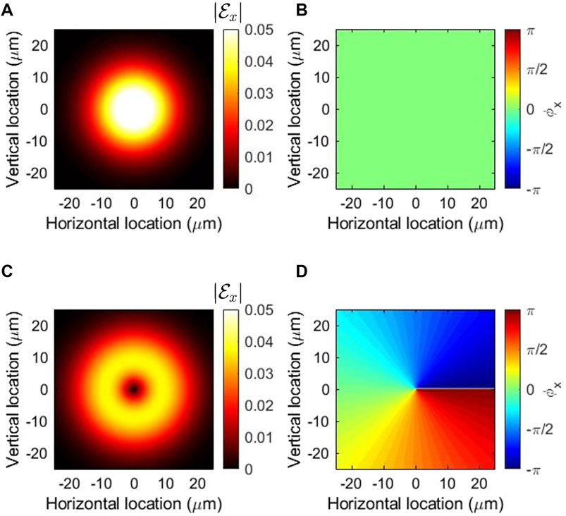
FIGURE 1. Ladder operation to increment the quantum number for orbital angular momentum. (A) The amplitude and (B) the phase of the input Gaussian beam without a vortex. (C) The amplitude and (D) the phase of the output beam after the ladder operation. The left vortex with topological charge of 1 is generated upon the ladder operation.
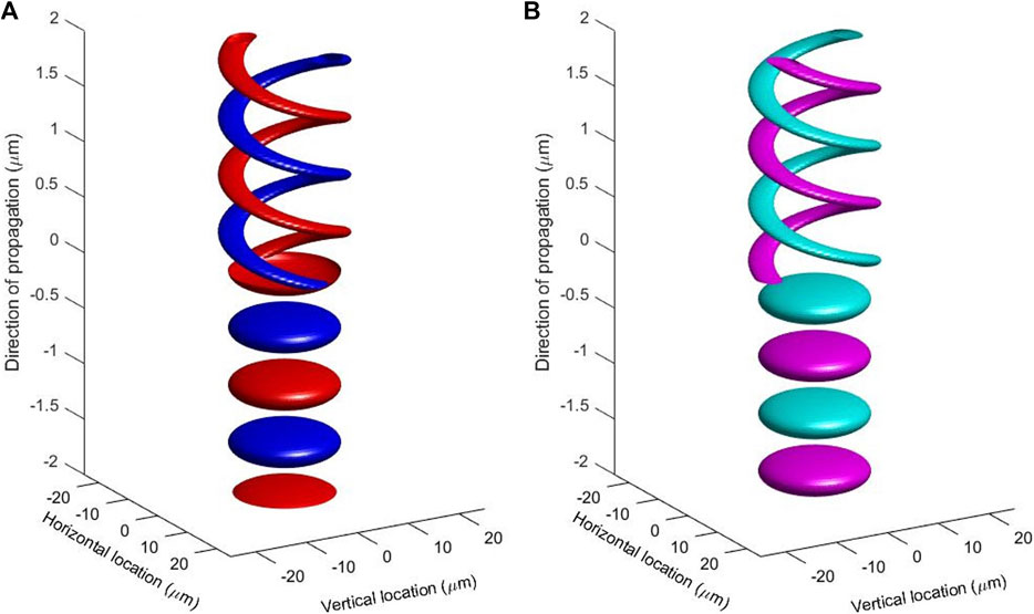
FIGURE 2. Generation of the left vortex upon passing through a vortex lens. The vortex lens was assumed to be located at z = 0, where the Gaussian input beam is converted to be the left vortex. (A) Real part and (B) imaginary part of the complex electric field,
We have also confirmed the generation of the left vortex along the direction of the propagation (Figure 2). We have assumed the same parameters to calculate the mode profiles in Figure 1, and considered that a vortex lens [5, 23, 59–61, 67, 69–73], is located at the middle of the direction of the propagation (z) at z = 0. In the calculation, we have used the ladder operation of
5.9 Extension and limitation of the theory
So far, we have discussed applications of canonical orbital angular momentum operators to Laguerre-Gauss modes in a GRIN fibre, and found that the ladder operations worked properly and analytically calculated the magnitude of orbital angular momentum. This is consistent with a view that orbital angular momentum is a well-defined quantum observable at least in a GRIN fibre. However, if orbital angular momentum is properly defined only in a GRIN fibre, applications of the present theory is limited. Finally, we discuss about the possibility to extend our theory for a more generic case and its limitation.
The reason why we have considered the GRIN fibre is that we can treat Laguerre-Gauss modes virtually exactly within the paraxial approximation. This allows us to consider the collimated beam, propagating in the GRIN fibre, for the fixed waist, w0. The GRIN fibre contains a limit of a uniform material at g = 0, where the most important application would be the vacuum at n0 = 1. In the vacuum, however, we need to consider the propagation dependent waist of w = w(z) and the spherical beam radius of R = R(z), as we derived in Section 2.4. It is also important to consider the Gouy phase [5, 42, 46–50]. These factors will add extra contributions during the applications of ladder operations. Fortunately, these extra contributions are negligible for the sufficiently large confocal parameter, known also as Rayleigh length,
Finally, we would like to discuss briefly whether our theory can applicable to other families of structured light, such as Hermite-Gauss [5, 9], Bessel-Gauss [74–77], and Ince-Gauss [78] beams. The Bessel-Gauss beams are quite attractive, since it prevents the diffraction and the mode shape is preserved upon propagation [74–77]. It is beyond the scope of the present work to develop ladder operations to these special functions in general rather than Laguerre-Gauss beams, but Laguerre-Gauss beams have correlation to Hermite-Gauss beams [5, 9]. The Hemite-Gauss beams in the GRIN fibre is given by
where Hl(x) and Hm(y) are Hermite functions with l and m as quantum numbers for horizontal and vertical directions [5, 9]. We are interested in the relationship to the Laguerre-Gauss beams
where σi (i = 1, 2, 3) is the Pauli matrix, and the commutation relationship becomes
where ϵijk is a complete anti-symmetric tensor. Then, we obtain the horizontal state in orbital angular momentum state as
where we have used the formula of r (eimϕ + e−imϕ) = 2r cos(ϕ) = 2x. This means that the Laguerre-Gauss beam is converted into the Hermite-Gauss beam [5]. Similarly, the vertical state in orbital angular momentum becomes
where we have used the formula of r (−eimϕ + e−imϕ) = −2ir sin(ϕ) = −i2y. Therefore, both horizontal and vertical states in orbital angular momentum are described by Hermite-Gauss beams [5]. We can calculate the average orbital angular momentum per a photon as
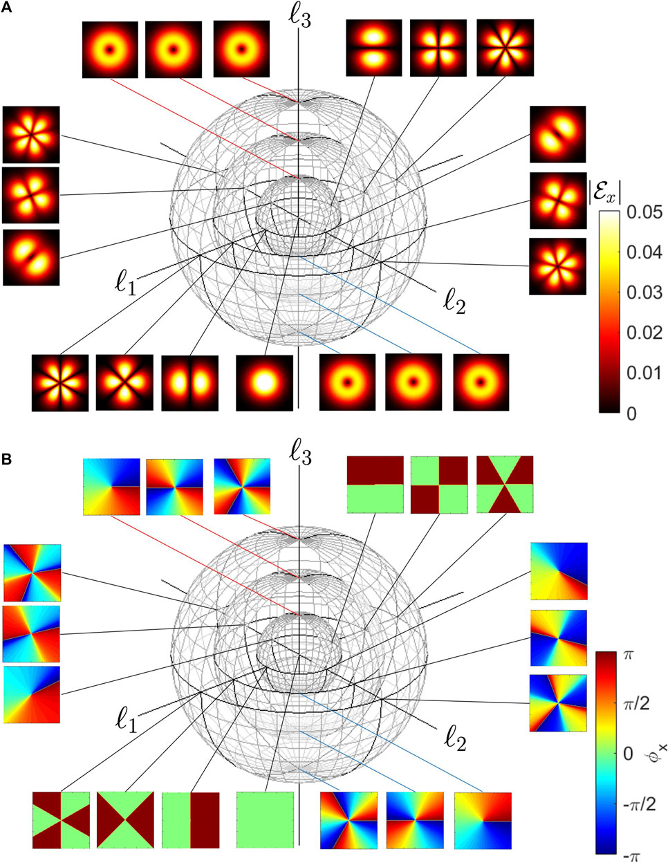
FIGURE 3. The higher-order Poincaré sphere for orbital angular momentum. By considering the superposition states between the left and the right vortexed states with topological charge of m and −m, respectively, the expectation values of the orbital angular momentum, (ℓ1, ℓ2, ℓ3), are calculated, which form the sphere with the radius of ℏm per a photon. (A) The amplitude and (B) the phase of superposition states are calculated at typical points. The ladder operators of
6 Conclusion
A photon, an elementary particle with the internal spin degree of freedom, can have an orbital degree of freedom [5, 6, 8–13]. In a vacuum, a photon travels at the speed of light, c, and is described by a plane wave [10]. The many-body state for photons can be described by a QED theory [1, 4, 11, 12, 44]. On the other hand, for a photon confined to a region with a larger refractive index, i.e., a waveguide, the mode is described as a confined mode, which is a bound state with a discrete energy level. The nature of this mode is completely different from that described by a plane wave allowing a continuous energy spectrum. We have shown that the fundamental equation to describe the orbital wavefunction of photons in a waveguide is Helmholtz equation [9, 10] for a monochromatic coherent beam emitted from a laser, where the spin degree of freedom is described by a Jones vector. We must solve the Helmholtz equation in a material including the refractive index profile and the symmetry of the system [88]. The reason why the many-body photonic state can be described by a single wavefunction is based on the Bose-Einstein condensation nature of a coherent state that allows a macroscopic number of photons to occupy the lowest energy state, because of the Bose statistics due to the integer spin. As a specific example, we have considered a GRIN fibre with a cylindrical symmetry, for which we could solve the Helmholtz equation exactly by using LG modes [5, 6, 8–12].
We have defined canonical OAM operators in cylindrical coordinates and have applied them to the LG modes. We have confirmed that the OAM is quantised along the direction of propagation and that the quantum-mechanical expectation value is indeed obtained as ℏm, while the average values along the directions perpendicular to the propagation vanish. We have found that the ladder operators to increase or decrease m work successfully to increment or decrement in units of ℏ. We could also calculate the quantum-mechanical average of the magnitude of OAM as a function of the radial quantum numbers of n and m. We have also confirmed the contributions from the intrinsic OAM and the origin-dependent extrinsic OAM. Finally, we have calculated the matrix elements of the ladder operators and have confirmed that the angular momentum operators are observable at least in the Hilbert space spanned by the LG modes. From those results, we conclude that the OAM is a proper quantum-mechanical degree of freedom and that a standard quantum-mechanical treatment is applicable to a monochromatic coherent beam of photons.
Data availability statement
The original contributions presented in the study are included in the article, further inquiries can be directed to the corresponding author.
Author contributions
The author confirms being the sole contributor of this work and has approved it for publication.
Funding
This work is supported by JSPS KAKENHI Grant Number JP 18K19958.
Acknowledgments
The author would like to express sincere thanks to Prof I. Tomita for continuous discussions and encouragements.
Conflict of interest
Author SS was employed by Hitachi, Ltd.
Publisher’s note
All claims expressed in this article are solely those of the authors and do not necessarily represent those of their affiliated organizations, or those of the publisher, the editors and the reviewers. Any product that may be evaluated in this article, or claim that may be made by its manufacturer, is not guaranteed or endorsed by the publisher.
References
5. Allen L, Beijersbergen MW, Spreeuw RJC, Woerdman JP. Orbital angular momentum of light and the transformation of Laguerre-Gaussian laser modes. Phys Rev A (1992) 45:8185–9. doi:10.1103/PhysRevA.45.8185
6. v Enk SJ, Nienhuis G. Commutation rules and eigenvalues of spin and orbital angular momentum of radiation fields. J Mod Opt (1994) 41:963–77. doi:10.1080/09500349414550911
7. Leader E, Lorcé C. The angular momentum controversy: What’s it all about and does it matter? Phys Rep (2014) 541:163–248. doi:10.1016/j.physrep.2014.02.010
8. Barnett SM, Allen L, Cameron RP, Gilson CR, Padgett MJ, Speirits FC, et al. On the natures of the spin and orbital parts of optical angular momentum. J Opt (2016) 18:064004. doi:10.1088/2040-8978/18/6/064004
9. Yariv Y, Yeh P. Photonics: Optical electronics in modern communications. Oxford: Oxford University Press (1997).
11. Grynberg G, Aspect A, Fabre C. Introduction to quantum optics: From the semi-classical approach to quantized light. Cambridge: Cambridge University Press (2010).
12. Bliokh KY, Rodríguez-Fortuño FJ, Nori F, Zayats AV. Spin-orbit interactions of light. Nat Photon (2015) 9:796–808. doi:10.1038/NPHOTON.2015.201
13. Al-Attili AZ, Burt D, Li Z, Higashitarumizu N, Gardes F, Ishikawa Y, et al. Chiral germanium micro-gears for tuning orbital angular momentum. Sci Rep (2022) 12:7465. doi:10.1038/s41598-022-11245-1
14. Allen L, Padgett MJ. The poynting vector in Laguerre-Gaussian beams and the interpretation of their angular momentum density. Opt Comm (2000) 184:67–71. doi:10.1016/S0030-4018(00)00960-3
15. Ji X. Comment on “Spin and orbital angular momentum in gauge theories: Nucleon spin structure and multipole radiation revisited”. Phys Rev Lett (2010) 104:039101. doi:10.1103/PhysRevLett.104.039101
16. Chen XS, Lü XF, Sun WM, Wang F, Goldman T. Spin and orbital angular momentum in gauge theories: Nucleon spin structure and multipole radiation revisited. Phys Rev Lett (2008) 100:232002. doi:10.1103/PhysRevLett.100.232002
17. Yang LP, Khosravi F, Jacob Z. Quantum field theory for spin operator of the photon. Phys Rev Res (2022) 4:023165. doi:10.1103/PhysRevResearch.4.023165
18. Forbes A, d Oliveira M, Dennis MR. Structured light. Nat Photon (2021) 15:253–62. doi:10.1038/s41566-021-00780-4
19. Nape I, Sephton B, Ornelas P, Moodley C, Forbes A. Quantum structured light in high dimensions. APL Photon (2023) 8:051101. doi:10.1063/5.0138224
20. Ma M, Lian Y, Wang Y, Lu Z. Generation, transmission and application of orbital angular momentum in optical fiber: A review. Front Phys (2021) 9:773505. doi:10.3389/fphy.2021.773505
21. Rosen GFQ, Tamborenea PI, Kuhn T. Interplay between optical vortices and condensed matter. Rev Mod Phys (2022) 94:035003. doi:10.1103/RevModPhys.94.035003
22. Shen Y, Rosales-Guzmán C. Nonseparable states of light: From quantum to classical. Laser Photon Rev (2022) 16:2100533. doi:10.1002/lpor.202100533
23. Cisowski C, Götte JB, Franke-Arnold S. Colloquium: Geometric phases of light: Insights from fiber bundle theory. Rev Mod Phys (2022) 94:031001. doi:10.1103/revmodphys.94.031001
24. Liu R, Zhang J, Liu J, Lin Z, Li Z, Lin Z, et al. 1-pbps orbital angular momentum fibre-optic transmission. Light Sci Appl (2022) 11:202. doi:10.1038/s41377-022-00889-3
25. Spreeuw BJC. A classical analogy of entanglement. Found Phys (1998) 28:361–74. doi:10.1023/A:1018703709245
26. Shen Y. Rays, waves, su(2) symmetry and geometry: Toolkits for structured light. J Opt (2021) 23:124004. doi:10.1088/2040-8986/ac3676
27. Saito S. Poincaré rotator for vortexed photons. Front Phys (2021) 9:646228. doi:10.3389/fphy.2021.646228
28. Saito S. Spin of photons: Nature of polarisation (2023). arXiv (2023) 2303.17112. doi:10.48550/arXiv.2303.17112
29. Saito S. SU(2) symmetry of coherent photons and application to poincaré rotator (2023). arXiv (2023) 2303.18199. doi:10.48550/arXiv.2303.18199
30. Saito S. Macroscopic singlet, triplet, and colour-charged states of coherent photons (2023). arXiv (2023) 2304.01216. doi:10.48550/arXiv.2304.01216
33. Gil JJ, Ossikovski R. Polarized light and the mueller matrix approach. London: CRC Press (2016). doi:10.1201/b19711
34. Kawakami S, Nishizawa J. An optical waveguide with the optimum distribution of the refractive index with reference to waveform distortion. IEEE Trans Microw Theor Techn. (1968) 16:814–8. doi:10.1109/TMTT.1968.1126797
35. Joannopoulos JD, Johnson SG, Winn JN, Meade RD. Photonic crystals: Molding the flow og light. New York: Princeton Univ. Press (2008).
36. Sotto M, Tomita I, Debnath K, Saito S. Polarization rotation and mode splitting in photonic crystal line-defect waveguides. Front Phys (2018) 6:85. doi:10.3389/fphy.2018.00085
37. Sotto M, Debnath K, Khokhar AZ, Tomita I, Thomson D, Saito S. Anomalous zero-group-velocity photonic bonding states with local chirality. J Opt Soc Am B (2018) 35:2356–63. doi:10.1364/JOSAB.35.002356
38. Sotto M, Debnath K, Tomita I, Saito S. Spin-orbit coupling of light in photonic crystal waveguides. Phys Rev A (2019) 99:053845. doi:10.1103/PhysRevA.99.053845
39. Bliokh KY, Bekshaev AY, Nori F. Optical momentum, spin, and angular momentum in dispersive media. Phys Rev Lett (2017) 119:073901. doi:10.1103/PhysRevLett.119.073901
40. Bliokh KY, Bekshaev AY, Nori F. Optical momentum and angular momentum in complex media: From the abraham-minkowski debate to unusual properties of surface plasmon-polaritons. New J Phys (2017) 19:123014. doi:10.1088/1367-2630/aa8913
41. Barnett SM, Babiker M, Padgett MJ. Optical orbital angular momentum. Phil Trans R Soc A (2016) 375:20150444. doi:10.1098/rsta.2015.0444
42. Simon R, Mukunda N. Bargmann invariant and the geometry of the Güoy effect. Phys Rev Lett (1993) 70:880–3. doi:10.1103/PhysRevLett.70.880
43. Lloyd SM, Babiker M, Thirunavukkarasu G, Yuan Y. Electron vortices: Beams with orbital angular momentum. Rev Mod Phys (2017) 89:035004. doi:10.1103/RevModPhys.89.035004
45. Schrieffer JR. Theory of superconductivity. Boca Raton: CRC Press (1971). doi:10.1201/9780429495700
46. Pancharatnam S. Generalized theory of interference, and its applications. Proc Indian Acad Sci Sect A (1956) XLIV:247–62. doi:10.1007/BF03046050
47. Berry MV. Quantual phase factors accompanying adiabatic changes. Proc R Sco Lond A (1984) 392:45–57. doi:10.1098/rspa.1984.0023
48. Tomita A, Cao RY. Observation of Berry’s topological phase by use of an optical fiber. Phys Rev Lett (1986) 57:937–40. doi:10.1103/PhysRevLett.57.937
49. Hamazaki J, Mineta Y, Oka K, Morita R. Direct observation of gouy phase shift in a propagating optical vortex. Opt Exp (2006) 14:8382–92. doi:10.1364/OE.14.008382
50. Bliokh K. Geometrodynamics of polarized light: Berry phase and spin Hall effect in a gradient-index medium. J Opt A: Pure Appl Opt (2009) 11:094009. doi:10.1088/1464-4258/11/9/094009
51. Nambu Y. Quasi-particles and gauge invariance in the theory of superconductivity. Phys Rev (1960) 117:648–63. doi:10.1103/PhysRev.117.648
52. Anderson PW. Random-phase approximation in the theory of superconductivity. Phys Rev (1958) 112:1900–16. doi:10.1103/PhysRev.112.1900
53. Goldstone J, Salam A, Weinberg S. Broken symmetries. Phy Rev (1962) 127:965–70. doi:10.1103/PhysRev.127.965
54. Higgs PW. Broken symmetries and the masses of gauge bosons. Phys Lett (1962) 12:508–9. doi:10.1103/PhysRevLett.13.508
55. Saito S. Dirac equation for photons: Origin of polarisation (2023). arXiv (2023) 2303.18196. doi:10.48550/arXiv.2303.18196
57. Whittaker ET, Watson GN. A course of modern analysis. Cambridge: Cambridge University Press (1962). doi:10.1017/9781009004091
58. Bateman H. Higher transcendental functions [volumes I-III]. New York: MacGraw-Hill Book Company (1953).
59. Padgett MJ, Courtial J. Poincaré-sphere equivalent for light beams containing orbital angular momentum. Opt Lett (1999) 24:430–2. doi:10.1364/OL.24.000430
60. Milione G, Sztul HI, Nolan DA, Alfano RR. Higher-order poincaré sphere, Stokes parameters, and the angular momentum of light. Phys Rev Lett (2011) 107:053601. doi:10.1103/PhysRevLett.107.053601
61. Liu Z, Liu Y, Ke Y, Liu Y, Shu W, Luo H, et al. Generation of arbitrary vector vortex beams on hybrid-order Poincaré sphere. Photon Res (2017) 5:15–21. doi:10.1364/PRJ.5.000015
62. Marrucci L, Manzo C, Paparo D. Optical spin-to-orbital angular momentum conversion in inhomogeneous anisotropic media. Phys Rev Lett (2006) 96:163905. doi:10.1103/PhysRevLett.96.163905
63. Machavariani G, Lumer Y, Moshe I, Meir A, Jackel S. Efficient extracavity generation of radially and azimuthally polarized beams. Opt Lett (2007) 32:1468–70. doi:10.1364/OL.32.001468
64. Lai WJ, Lim BC, Phua PB, Tiaw KS, Teo HH, Hong MH. Generation of radially polarized beam with a segmented spiral varying retarder. Opt Exp (2008) 16:15694–9. doi:10.1364/OE.16.015694
65. Guan B, Scott RP, Qin C, Fontaine NK, Su T, Ferrari C, et al. Free-space coherent optical communication with orbital angular, momentum multiplexing/demultiplexing using a hybrid 3d photonic integrated circuit. Opt Exp (2013) 22:145–56. doi:10.1364/OE.22.000145
66. Sun J, Moresco M, Leake G, Coolbaugh D, Watts MR. Generating and identifying optical orbital angular momentum with silicon photonic circuits. Opt Lett (2014) 39:5977–80. doi:10.1364/OL.39.005977
67. Naidoo D, Roux FS, Dudley A, Litvin I, Piccirillo B, Marrucci L, et al. Controlled generation of higher-order Poincaré sphere beams from a laser. Nat Photon (2016) 10:327–32. doi:10.1038/NPHOTON.2016.37
68. Dorney KM, Rego L, Brooks NJ, San Román J, Liao CT, Ellis JL, et al. Controlling the polarization and vortex charge of attosecond high-harmonic beams via simultaneous spin-orbit momentum conservation. Nat Photon (2019) 13:123–30. doi:10.1038/s41566-018-0304-3
69. Erhard M, Fickler R, Krenn M, Zeilinger A. Twisted photons: New quantum perspectives in high dimensions. Light: Sci Appl (2018) 7:17146. doi:10.1038/lsa.2017.146
70. Andrews DL. Symmetry and quantum features in optical vortices. Symmetry (2021) 13:1368. doi:10.3390/sym.13081368
71. Angelsky OV, Bekshaev AY, Dragan GS, Maksimyak PP, Zenkova CY, Zheng J. Structured light control and diagnostics using optical crystals. Front Phys (2021) 9:715045. doi:10.3389/fphy.2021.715045
72. Agarwal GS. SU(2) structure of the poincaré sphere for light beams with orbital angular momentum. J Opt Soc A A (1999) 16:2914–6. doi:10.1364/JOSAA.16.002914
73. Golub MA, Shimshi L, Davidson N, Friesem AA. Mode-matched phase diffractive optical element for detecting laser modes with spiral phases. Appl Opt (2007) 46:7823–8. doi:10.1364/AO.46.007823
74. Gori F, Guattari G, Padovani C. Bessel gauss beams. Opt Commun (1987) 64:491–5. doi:10.1016/0030-4018(87)90276-8
75. Durnin J, Miceli JJJ, Eberly JH. Diffraction-free beams. Phys Rev Lett (1987) 58:1499–501. doi:10.1103/physrevlett.58.1499
76. Wang W, Ye T, Wu Z. Probability property of orbital angular momentum distortion in turbulence. Opt Exp (2021) 29:44157–73. doi:10.1364/OE.445175
77. Wang W, Zhang G, Ye T, Wu Z, Bai L. Scintillation of the orbital angular momentum of a bessel Gaussian beam and its application on multi-parameter multiplexing. Opt Exp (2023) 31:4507–20. doi:10.1364/OE.478127
78. Bandres MA, Gutiérrez-Vega JC. Ince-Gaussian beams. Opt Lett (2004) 29:144–6. doi:10.1364/OL.29.000144
79. Jones RC. A new calculus for the treatment of optical systems i. description and discussion of the calculus. J Opt Soc Am (1941) 31:488–93. doi:10.1364/JOSA.31.000488
81. Born M, Wolf E. Principles of optics. Cambridge: Cambridge University Press (1999). doi:10.1017/9781108769914
82. Collett E. Stokes parameters for quantum systems. Am J Phys (1970) 38:563–74. doi:10.1119/1.1976407
83. Luis A. Degree of polarization in quantum optics. Phys Rev A (2002) 66:013806. doi:10.1103/PhysRevA.66.013806
84. Luis A. Polarization distributions and degree of polarization for quantum Gaussian light fields. Opt Comm (2007) 273:173–81. doi:10.1016/j.optcom.2007.01.016
85. Björk G, Söderholm J, Sánchez-Soto LL, Klimov AB, Ghiu I, Marian P, et al. Quantum degrees of polarization. Opt Comm (2010) 283:4440–7. doi:10.1016/j.optcom.2010.04.088
86. d Castillo Gft , García IR. The Jones vector as a spinor and its representation on the Poincaré sphere. Rev Mex Fis (2011) 57:406–13. doi:10.48550/arXiv.1303.4496
87. Al-Attili AZ, Kako S, Husain MK, Gardes FY, Higashitarumizu N, Iwamoto S, et al. Whispering gallery mode resonances from ge micro-disks on suspended beams. Front Mat (2015) 2:43. doi:10.3389/fmats.2015.00043
88. Saito S, Tomita I, Sotto M, Debnath K, Byers J, Al-Attili AZ, et al. Si photonic waveguides with broken symmetries: Applications from modulators to quantum simulations. Jpn J Appl Phys (2020) 59:SO0801. doi:10.35848/1347-4065/ab85ad
90. Hall BC. Lie groups, Lie algebras, and representations; an elementary introduction. Switzerland: Springer (2003).
92. Georgi H. Lie algebras in particle physics: From isospin to unified theories (Frontiers in physics). Massachusetts: Westview Press (1999).
Keywords: orbital angular momentum, commutation relationship, ladder operator, Laguerre-Gauss mode, graded index fibre, coherent state
Citation: Saito S (2023) Quantum commutation relationship for photonic orbital angular momentum. Front. Phys. 11:1225346. doi: 10.3389/fphy.2023.1225346
Received: 19 May 2023; Accepted: 26 July 2023;
Published: 13 October 2023.
Edited by:
Carmelo Rosales-Guzmán, Centro de Investigaciones en Optica, MexicoReviewed by:
Roberto Ramirez Alarcon, Centro de Investigaciones en Optica, MexicoYijie Shen, University of Southampton, United Kingdom
Copyright © 2023 Saito. This is an open-access article distributed under the terms of the Creative Commons Attribution License (CC BY). The use, distribution or reproduction in other forums is permitted, provided the original author(s) and the copyright owner(s) are credited and that the original publication in this journal is cited, in accordance with accepted academic practice. No use, distribution or reproduction is permitted which does not comply with these terms.
*Correspondence: Shinichi Saito, c2hpbmljaGkuc2FpdG8ucXRAaGl0YWNoaS5jb20=