Analysis and numerical approximation of the fractional-order two-dimensional diffusion-wave equation

Non-local fractional derivatives are generally more effective in mimicking real-world phenomena and offer more precise representations of physical entities, such as the oscillation of earthquakes and the behavior of polymers. This study aims to solve the 2D fractional-order diffusion-wave equation using the Riemann–Liouville time-fractional derivative. The fractional-order diffusion-wave equation is solved using the modified implicit approach based on the Riemann–Liouville integral sense. The theoretical analysis is investigated for the suggested scheme, such as stability, consistency, and convergence, by using Fourier series analysis. The scheme is shown to be unconditionally stable, and the approximate solution is consistent and convergent to the exact result. A numerical example is provided to demonstrate that the technique is more workable and feasible.

1 Introduction

Fractional calculus is the non-integer or fractional-order differentiation and integration that has received significant attention over the last two decades for its application in describing real-world problems. Non-linear fractional-order differential equations (NL-FDEs) play a major role in applied sciences and social sciences, such as material science, signal processing, control theory, finance, and food supplements [1–3]. Recently, many advanced and reliable approaches have been discussed by the researchers. For example, Shen et al. [4] discussed the analytical and numerical solutions for a 2D multi-term time-fractional DWE. They used the approach of the variable of separation to drive analytical solutions, as well as the properties of Mittag–Leffler functions, and showed that stability and convergence analyses were studied. Ruzhansky et al. [5] considered the multi-term DWE and used the Caputo derivative, a non-local initial problem, and the Mittag–Leffler function in this study. Fan et al. [6] investigated the inverse problem to recognize the initial value for the space–time FDWE. They utilized the Landweber iterative regularization method for the time–space FDWE and calculated the error between validity and stability. The approximate solutions for 1D and 2D multi-term time-fractional sub-diffusion and DWEs with smooth and non-smooth solutions have been discussed by Rashidinia et al. [7]. They applied the Legendre collocation method and the Caputo derivative for solving the proposed equation. Moreover, they found the convergence analysis and concluded that this method has the benefit of using limited Legendre polynomials to obtain accurate and acceptable results. Feng et al. [8] researched a novel approach based on the finite element method (FEM) 2D diffusion type non-integer order equation. The utilized scheme is approximated for three different types of equations. The matrix form of the scheme is generated using the FEM, and the formulation of the equation is determined. The theoretical analysis, such as stability and convergence, is established. The suggested technique is versatile and resilient and may be used to solve various multi-term time-fractional diffusion problems directly. The Caputo derivative is in the temporal direction of the 2D time-dependent FDWE, as studied by Yang et al [9]. They used the finite difference method (FDM) to discretize the fractional-order derivative and provide a meshless approximation in spatial directions using moving least squares (MLS), which may be used to solve more complicated problem domains. The study also investigated the time-related convergence and stability properties of the semi-discretized scheme. In another study, Yang et al. [9] considered a 2D non-linear time-fractional DWE solved using a Crank–Nicolson Legendre spectral technique. The time-stepping is performed using the Crank–Nicolson difference method, while the spatial discretization is performed using the Legendre spectral approach. Lyu et al. [10] suggested a fast and linearized FDM for solving the non-linear multi-term FDWE. The suggested technique is based on a weighted approach, fast $L_2-1_{\sigma }$ discretization, and multi-term $L_2-1_{\sigma }$-type discretization. The obtained truncation error in the suggested weighted discretization to the multi-term Caputo derivative rigorously proved unconditional convergence by demonstrating certain crucial aspects of the refined coefficients of full discretization. Salehi [11] investigated multi-term FDWS in 2D and solved it using a meshless collocation approach. The shape functions for spatial approximation are constructed using the moving least squares reproducing kernel particle approximation. They also created a semi-discrete technique by discretizing Caputo’s time derivatives using a finite difference approximation. The obtained difference schemes demonstrated unconditional stability and convergence. Ghafoor et al. [12] developed a technique based on the approximations of finite difference and Haar wavelets. The approach is used to numerically solve $\left(1+1\right)$-D and $\left(1+2\right)$-D time fractional PDEs. Zhuang and Liua [13] worked on a finite domain and the 2D temporal fractional diffusion equation (2D-TFDE). The 2D-TFDE is modeled using an implicit difference approximation. The mathematical induction approach is used to assess the stability and convergence analysis. Heydari et al. [14] investigated the approximate solution to the variable-order (VO) space–time fractional non-linear diffusion-wave problem. The established approach combines the collocation and tau methods with the Chebyshev cardinal functions and their operational matrix of VO-FDs. A resilient and reliable numerical approach for solving a 2D VO non-linear FDWE on arbitrary domains was suggested by Shekari et al. [15] using the MLS meshless procedure for the space domain and the FDS for the time domain . The method was devised in such a way that it is independent of the uniformity of the domain in consideration and the solution of the algebraic system of equations. The proposed method was tested using a variety of space domains, including quadrilateral, rounded, triangular, and polar domains, as well as different types of non-linearity. Kumar et al. [16]provided the local collocation method that depends on radial basis functions to investigate the solution of time-fractional non-linear DWEs. They demonstrated the numerical schemes that are unconditionally stable and converge in semi-discrete. Ding [17] researched the creation of a high-order numerical approach for the 2D time-space FDWEs. A new approach with order $O\left({\tau }^2+h^4+h^4\right)$ is derived based on the fourth-order fractional-compact difference operator, where the temporal step size\tau and $h_1$ and $h_2$ are the spatial step sizes, respectively. The energy approach is used to analyze the algorithm’s stability and convergence, and a numerical experiment is conducted to confirm the numerical algorithm’s viability. Li et al. [18] analyzed a 2D non-linear FDWE in both time and space. The spatial component is discretized using the Galerkin FEM, while the temporal part is discretized using the new ADI method,” which also proved stability and convergence. They presented a 2D FDWE with the fractional derivative of order $\alpha \left(1<\alpha <2\right)$. Li et. al. [19] considered the ADI analysis based on the Crank–Nicolson method and the Galerkin FEM, both of which are analyzed. The ADI scheme is unconditionally stable, and $L_2$ norm convergence is rigorously illustrated. Datsko et al. [20] proposed that the TFDE with mass absorption in a sphere is observed under the harmonic impact on the surface of a sphere. The TFD of “Caputo” is implemented. The Mittag–Leffler function is also used to express the Laplace transform with respect to time and the finite sin-Fourier transform with respect to the spatial coordinates. Ren and Sun [21] discussed the fourth-order compact algorithm for solving the TFDWE with Neumann boundary conditions. For the time-fractional derivative, $L_1$ discretization is used, whereas the compact difference methodology is used for spatial discretization. The compact difference scheme is unconditionally stable, and global convergence is carefully shown. In addition, the Crank–Nicolson scheme with second-order spatial precision is described and perhaps an error estimate as well. The 2D case is solved using the compact ADI difference algorithm with Robin boundary conditions. Yang et al. [22] considered the initial value problem with mixed initial conditions of TFDWEs. They used the truncated regularization method and investigated conditional stability and error approximations, as well as some acceptable numerical examples, to establish the method’s validity. The convergence estimates in this publication are not saturated when compared with other authors’ works, and the non-homogeneous factors are correlated. Ali and Abdullah [23] discussed the FDWEs of arbitrary order.” They explain efficiency and fruitfulness through numerical test examples. There are many related studies available in the literature discussing different types of fractional-order models. For instance, Nawaz et al. [24] considered two numerical approaches, found the solution for two fractional-order models, and compared their solution with classical solutions. The fractional-order operator is in the Caputo sense, and we obtained the results numerically and graphically. They claimed that the methods are quickly convergent and yield encouraging results. Farid et al. [25] examined the Laplace transform with an iterative method for the space–time fractional-order models. They compared the obtained results with other existing schemes in the literature, which are more feasible and effective. Sayevand and Jafari [26] introduced the fractional-order KdV model in a fractal domain and applied the transformation to convert the fractional order into an ordinary-order derivative. They analyzed the theoretical analyses and presented many numerical examples to confirm the accuracy of the suggested approach. Li et al. [27] studied the significant properties of the Caputo fractional derivative in the real line and further developed it in the complex plane, which is used in signal processing. Guariglia [28] derived the functional equation for the fractional-order derivative Hurwitz function and proved the relation between the fractional-order zeta function and Bernoulli numbers. In another study, Guariglia [29] presented the functional equation with the Grunwald–Letnikov fractional derivative and discussed the link with the distribution of prime numbers. The other comprehensive literature can be studied in [30–37].

According to the previously described literature, fractional calculus is still a relatively new field that requires more accurate numerical approaches to examine the more practicable FDEs. The goal of this research is to develop a more accurate and reliable numerical technique for the FDWE. An attempt to discretize the R-L integral operator numerically and implement it in the Riemann–Liouville fractional-order derivative to approximate the FDWE has not yet been made. This approach reduces computational complexity and increases accuracy. Analysis, including aspects such as stability, consistency, and convergence, was also investigated based on the Fourier method and Taylor’s series expansion.

The remainder of the paper is arranged as follows: the associated preliminaries are described in Section 2. Section 3 explains the proposed method. The stability analysis is discussed in Section 4. Consistency and convergence are addressed in Section 5. Section 6 presents the numerical results, and the conclusion is provided in Section 7.

Here, we consider the FDWE as follows [23]:

$\frac{{\partial }^{2}w\left(x,y,t\right)}{\partial t^2}=D_t^{2-q}\left(\frac{{\partial }^{2}w\left(x,t\right)}{\partial x^2}+\frac{{\partial }^{2}w\left(y,t\right)}{\partial y^2}\right)+F\left(x,y,t\right),\hspace{1em}qϵ\left.\left(\mathrm{0,1}\right.\right],\hspace{1em}xϵ\left[0,L\right],\hspace{1em}yϵ\left[0,L\right],\hspace{1em}tϵ\left[0,T\right],(1)$

where the conditions are

$w\left(x,y,0\right)={\phi }_1\left(x,y\right),w_t\left(x,y,0\right)={\phi }_2\left(x,y\right),(2)$

$w\left(0,y,t\right)={\phi }_3\left(y,t\right),w\left(L,y,t\right)={\phi }_4\left(y,t\right),w\left(x,0,t\right)={\phi }_5\left(x,t\right),w\left(x,L,t\right)={\phi }_6\left(x,t\right),(3)$

where $F\left(x,y,t\right)$ represents the non-homogenous term and $D_t^{2-q}$ denotes the R-L fractional-order derivative operator of order $q$ lying between 0 and 1.

2 Preliminaries

The R-L fractional differential operator is the most important extension of the classical differential operator. The R-L fractional-order derivative is defined as follows [38]:

$D_t^{2-q}w\left(x,y,t\right)=\frac{1}{\begin{array}{c}\mathrm{\Gamma }\left(\mathrm{q}\right)\end{array}}\frac{d^2}{d{t}^2}{\displaystyle {\int }_0^t}\frac{w\left(x,y,z\right)}{{\left(t-z\right)}^{1-q}}dz=\frac{d^2}{d{t}^2}{I}_0^{q}w\left(x,y,t\right).(4)$

The R-L integral operator can be defined as follows:

$I_0^{q}w\left(x,y,t\right)=\frac{1}{\mathrm{\Gamma }\left(\mathrm{q}\right)}{\int }_0^t\frac{w\left(x,y,z\right)}{{\left(t-z\right)}^{1-q}}dz,(5)$

where $I_0^q$ represents the R-L fractional-order integral operator of order $q$ lying between 0 and 1. Equation 5 can also be written as

$I_0^{q}w\left(x,y,t_n\right)=\frac{1}{\mathrm{\Gamma }\left(q\right)}{\int }_0^{t_n}{\left(t_n-z\right)}^{q-1}w\left(x,y,z\right)dz.(6)$

We use the Jumarie property in [25] as

$=\frac{1}{q\mathrm{\Gamma }\left(q\right)}{\displaystyle {\int }_0^{t_n}}W\left(x,y,z\right){\left(dz\right)}^q.$

By discretization of the aforementioned equation, we obtain the following equations:

$=\frac{1}{\mathrm{\Gamma }\left(1+q\right)}{\displaystyle {\sum }_{k=0}^{n-1}}{\int }_{t_k}^{t_{k+1}}w\left(x,y,z\right){\left(dz\right)}^q,=\frac{1}{\mathrm{\Gamma }\left(1+q\right)}{\displaystyle {\sum }_{k=0}^{n-1}}w\left(x,y,t_{n-k}\right){\int }_{t_k}^{t_{k+1}}{z}^0{\left(dz\right)}^q.(7)$

Applying the Jumarie property ${\int }_0^t{z}^m{\left(dz\right)}^n=\left(\frac{\mathrm{\Gamma }\left(1+m\right)\mathrm{\Gamma }\left(1+n\right)}{\mathrm{\Gamma }\left(1+m+n\right)}\right)t^{m+n}$,

$=\frac{{\tau }^q}{\mathrm{\Gamma }\left(1+q\right)}{\displaystyle {\sum }_{k=0}^{n-1}}w(x,y,t_{n-k})\left({\left(k+1\right)}^q-{\left(k\right)}^q\right),=\frac{{\tau }^q}{\mathrm{\Gamma }\left(1+q\right)}{\displaystyle {\sum }_{k=0}^{n-1}}{C}_k^{q}w\left(x,y,t_{n-k}\right),(8)$

where $\Delta t=\tau$ is the time step and can be defined as $t_{k+1}=\left(\left(k+1\right)\Delta t\right)=\left(\left(k+1\right)\tau \right)$ and $C_k^{\left(q\right)}={\left(k+1\right)}^q-{\left(k\right)}^q$, where $k=0,1,2,\dots ,n-1$.

Lemma 1. The $q\left(0<q<1\right)$-order R-L fractional integral of $w\left(x,y,t\right)$ in $\left[0,T\right]$ is defined as

$I_0^{q}w\left(x_i,y_j,t_k\right)=\frac{{\tau }^q}{\mathrm{\Gamma }\left(1+q\right)}{\displaystyle {\sum }_{v=0}^{k-1}}{C}_v^{\left(q\right)}w\left(x_i,y_j,t_{k-v}\right).(9)$

Lemma 2. The coefficient $C_k^{\left(q\right)}\left(k=\mathrm{0,1,2}\dots \right)$ satisfies the following properties [39]:

$•C_0^{\left(q\right)}=1,C_k^{\left(q\right)}>0,\hspace{1em}k=\mathrm{0,1},\dots .,$

$•C_{k-1}^{\left(q\right)}>C_k^{\left(q\right)},\hspace{1em}k=\mathrm{1,2},\dots .,$

$•\tau \le C_1{C}_k^{\left(q\right)}{\tau }^q,\hspace{1em}where{C}_1>0,$

$•{\displaystyle \sum _{k=0}^n}{C}_k^{\left(q\right)}{\tau }^q={\left(n+1\right)}^q\le T^q.$

3 The proposed implicit difference scheme

In this section, the implicit difference scheme (IDS) for the FDWE is constructed using Lemma 1 for the fractional-order part, and the space-derivative is reduced to the central difference approximation. The step for space is $x_i=i\Delta x$ and $y_j=j\Delta \mathrm{y}$, and the step for time is $t_k=k\tau$, where 1 $\le i\le M-1,\Delta x=\frac{L}{M},\Delta y=\frac{V}{H},0\le k\le N,\text{and\hspace{0.17em}}\tau =\frac{T}{N}$, respectively. We substitute Eq. 2 in Eq. 1 at mesh point $w\left(x_i,y_j,t_k\right)$ as follows:

$\frac{{\partial }^{2}w\left(x_i,y_j,t_k\right)}{\partial t^2}=\frac{d^2}{d{t}^2}{I}_0^q\frac{{\delta }_x^{2}w\left(x_i,y_j,t_k\right)}{\Delta x^2}+\frac{d^2}{d{t}^2}{I}_0^q\frac{{\delta }_y^{2}w\left(x_i,y_j,t_k\right)}{\Delta y^2}+F\left(x_i,y_j,t_k\right).(10)$

To eliminate the second-order time derivatives, we applied the backward difference approximation, then integrated from $t_k$ to $t_{k+1}$, and also, used the trapezoidal rule for the forcing term. Finally, we obtained

$w_{i,j}^{k+1}-2w_{i,j}^k+w_{i,j}^{k-1}=\frac{I_0^q}{\Delta x^2}\left({\delta }_x^2{w}_{i,j}^{k+1}-2{\delta }_x^2{w}_{i,j}^k+{\delta }_x^2{w}_{i,j}^{k-1}\right)+\frac{I_0^q}{\Delta y^2}\left({\delta }_y^2{w}_{i,j}^{k+1}-2{\delta }_y^2{w}_{i,j}^k+{{\delta }_y^{2}w}_{i,j}^{k-1}\right)+\frac{{\tau }^2}{2}\left[F_{i,j}^{k+1}+F_{i,j}^k\right].(11)$

We substituted Lemma 1, and after simplification, we obtained the approximated scheme for the FDWE as follows:

$\begin{array}{ll}\hfill w_{i,j}^{k+1}-2w_{i,j}^k+w_{i,j}^{k-1}& =[S_1\left(w_{i+1,j}^{k+1}-2w_{i,j}^{k+1}+w_{i-1,j}^{k+1}\right)-S_1\left(w_{i+1,j}^k-2w_{i,j}^k+w_{i-1,j}^k\right)\hfill \\ \hfill & +{\displaystyle {\sum }_{v=0}^{k-1}}\left(C_{v+1}^q-C_v^q\right)\left(w_{i+1,j}^{k-v}-2w_{i,j}^{k-v}+w_{i-1,j}^{k-v}\right)-S_1{\displaystyle {\sum }_{v=1}^{k-1}}\left(C_v^q-C_{v-1}^q\right)\left(w_{i+1,j}^{k-v}-2w_{i,j}^{k-v}+w_{i-1,j}^{k-v}\right)]\hfill \\ \hfill & +[S_2\left(w_{i,j+1}^{k+1}-2w_{i,j}^{k+1}+w_{i,j-1}^{k+1}\right)-S_2\left(w_{i,j+1}^k-2w_{i,j}^k+w_{i,j-1}^k\right)\hfill \\ \hfill & +S_2{\displaystyle {\sum }_{v=0}^{k-1}}\left(C_{v+1}^q-C_v^q\right)\left(w_{i,j+1}^{k-v}-2w_{i,j}^{k-v}+w_{i,j-1}^{k-v}\right)-S_2{\displaystyle {\sum }_{v=0}^{k-1}}\left(C_v^q-C_{v-1}^q\right)\left(w_{i,j+1}^{k-v}-2w_{i,j}^{k-v}+w_{i,j-1}^{k-v}\right)]\hfill \\ \hfill & +\frac{{\tau }^2}{2}\left[F_{i,j}^{k+1}+F_{i,j}^k\right].\hfill \end{array}(12)$

We know that $w_t\left(x,y,0\right)={\phi }_2\left(x,y\right)$. Therefore,

$w_{i,j}^{-1}=w_{i,j}^1+2\tau {\phi }_2\left(x_i,y_j\right),(13)$

$w_{i,j}^0={\phi }_1\left(x_i,y_i\right),w_{0,j}^k=w_{M_x,j}^k=w_{0,j}^k=w_{0,{\mathrm{M}}_{\mathrm{y}}}^k=0,(14)$

where $S_1=\frac{{\tau }^q}{г\left(q+1\right){∆x}^2},S_2=\frac{{\tau }^q}{г\left(q+1\right){∆y}^2},i=1,2,\dots .M_x-1,j=1,2,\dots ,M_y-1,andk=1,2,\dots ,N-1.$

4 Stability

The von Neumann method is used to determine the stability of the proposed scheme, and the approach in [40]is followed. Let $w_{i,j}^k$ represent the exact solution for Eq. 12, and we obtain

$\begin{array}{ll}\hfill w_{i+1,j}^{k+1}-2w_{i,j}^{k+1}+w_{i-1,j}^{k+1}& =[S_1\left(w_{i+1,j}^{k+1}-2w_{i,j}^{k+1}+w_{i-1,j}^{k+1}\right)-S_1\left(w_{i+1,j}^k-2w_{i,j}^k+w_{i-1,j}^k\right)\hfill \\ \hfill & +S_1{\displaystyle {\sum }_{v=0}^{k-1}}\left(C_{v+1}^q-C_v^q\right)\left(w_{i+1,j}^{k-v}-2w_{i,j}^{k-v}+w_{i-1,j}^{k-v}\right)-S_1{\displaystyle {\sum }_{v=1}^{k-1}}\left(C_v^q-C_{v-1}^q\right)\left(w_{i+1,j}^{k-v}-2w_{i,j}^{k-v}+w_{i-1,j}^{k-v}\right)]\hfill \\ \hfill & +[S_2\left(w_{i,j+1}^{k+1}-2w_{i,j}^{k+1}+w_{i,j-1}^{k+1}\right)-S_2\left(w_{i,j+1}^k-2w_{i,j}^k+w_{i,j-1}^k\right)\hfill \\ \hfill & +S_2{\displaystyle {\sum }_{v=0}^{k-1}}\left(C_{v+1}^q-C_v^q\right)\left(w_{i,j+1}^{k-v}-2w_{i,j}^{k-v}+w_{i,j-1}^{k-v}\right)-S_2{\displaystyle {\sum }_{v=0}^{k-1}}\left(C_v^q-C_{v-1}^q\right)\left(w_{i,j+1}^{k-v}-2w_{i,j}^{k-v}+w_{i,j-1}^{k-v}\right)].\hfill \end{array}(15)$

The error is defined as $E_{i,j}^k=w_{i,j}^k-W_{i,j}^k$, and $E_{i,j}^k$ satisfies Eq. 15 as follows:

$\begin{array}{ll}\hfill E_{i+1,j}^{k+1}-2E_{i,j}^{k+1}+E_{i-1,j}^{k+1}& =[S_1\left(E_{i+1,j}^{k+1}-2E_{i,j}^{k+1}+E_{i-1,j}^{k+1}\right)-S_1\left(E_{i+1,j}^k-2E_{i,j}^k+E_{i-1,j}^k\right)\hfill \\ \hfill & +S_1{\displaystyle {\sum }_{v=0}^{k-1}}\left(C_{v+1}^q-C_v^q\right)\left(E_{i+1,j}^{k-v}-2E_{i,j}^{k-v}+E_{i-1,j}^{k-v}\right)-S_1{\displaystyle {\sum }_{v=1}^{k-1}}\left(C_v^q-C_{v-1}^q\right)\left(E_{i+1,j}^{k-v}-2E_{i,j}^{k-v}+E_{i-1,j}^{k-v}\right)]\hfill \\ \hfill & +[S_2\left(E_{i,j+1}^{k+1}-2E_{i,j}^{k+1}+E_{i,j-1}^{k+1}\right)-S_2\left(E_{i,j+1}^k-2E_{i,j}^k+E_{i,j-1}^k\right)+S_2{\displaystyle {\sum }_{v=0}^{k-1}}\left(C_{v+1}^q-C_v^q\right)\hfill \\ \hfill & \left(E_{i,j+1}^{k-v}-2E_{i,j}^{k-v}+E_{i,j-1}^{k-v}\right)-S_2{\displaystyle {\sum }_{v=0}^{k-1}}\left(C_v^q-C_{v-1}^q\right)\left(E_{i,j+1}^{k-v}-2E_{i,j}^{k-v}+E_{i,j-1}^{k-v}\right)\hfill \\ \hfill & S_2{\displaystyle {\sum }_{v=0}^{k-1}}\left(C_{v+1}^q-C_v^q\right)\left(E_{i,j+1}^{k-v}-2E_{i,j}^{k-v}+E_{i,j-1}^{k-v}\right)-S_2{\displaystyle {\sum }_{v=0}^{k-1}}\left(C_v^q-C_{v-1}^q\right)\left(E_{i,j+1}^{k-v}-2E_{i,j}^{k-v}+E_{i,j-1}^{k-v}\right)].\hfill \end{array}(16)$

We assume that the growth factor takes the form of a single Fourier mode as

$E_{i,j}^k={\lambda }^k{e}^{\sqrt{-1}\sigma \left(\Delta xi+\Delta yj\right)},(17)$

where $\sigma$ and $\Delta x$ and $\Delta y$ are the mode number and step sizes, respectively. Eq. 17 can be the solution of the aforementioned error in Eq. 16.

$\begin{array}{c}{\lambda }^{k+1}{e}^{\sqrt{-1}\left(i\Delta x{\sigma }_1+j\Delta y{\sigma }_2\right)}-2{\lambda }^k{e}^{\sqrt{-1}\left(i\Delta x{\sigma }_1+j\Delta y{\sigma }_2\right)}+{\lambda }^{k-1}{e}^{\sqrt{-1}\left(i\Delta x{\sigma }_1+j\Delta y{\sigma }_2\right)}\hfill \\ =[S_1\left({\lambda }^{k+1}{e}^{\sqrt{-1}\left(\left(i+1\right)\Delta x{\sigma }_1+j\Delta y{\sigma }_2\right)}-2{\lambda }^{k+1}{e}^{\sqrt{-1}\left(i\Delta x{\sigma }_1+j\Delta y{\sigma }_2\right)}+{\lambda }^{k+1}{e}^{\sqrt{-1}\left(\left(i-1\right)\Delta x{\sigma }_1+j\Delta y{\sigma }_2\right)}\right)\hfill \\ -S_1\left({\lambda }^k{e}^{\sqrt{-1}\left(\left(i+1\right)\Delta x{\sigma }_1+j\Delta y{\sigma }_2\right)}-2{\lambda }^k{e}^{\sqrt{-1}\left(i\Delta x{\sigma }_1+j\Delta y{\sigma }_2\right)}+e^{\sqrt{-1}\left(\left(i-1\right)\Delta x{\sigma }_1+j\Delta y{\sigma }_2\right)}\right)\hfill \\ +S_1{\displaystyle {\sum }_{v=0}^{k-1}}\left(C_{v+1}^q-C_v^q\right)\left({\lambda }^{k-v}{e}^{\sqrt{-1}\left(\left(i+1\right)\Delta x{\sigma }_1+j\Delta y{\sigma }_2\right)}-2{\lambda }^{k-v}{e}^{\sqrt{-1}\left(i\Delta x{\sigma }_1+j\Delta y{\sigma }_2\right)}+{\lambda }^{k-v}{e}^{\sqrt{-1}\left(\left(i-1\right)\Delta x{\sigma }_1+j\Delta y{\sigma }_2\right)}\right)\hfill \\ -S_1{\displaystyle {\sum }_{v=1}^{k-1}}\left(C_v^q-C_{v-1}^q\right)\left({\lambda }^{k-v}{e}^{\sqrt{-1}\left(\left(i+1\right)\Delta x{\sigma }_1+j\Delta y{\sigma }_2\right)}-2{\lambda }^{k-v}{e}^{\sqrt{-1}\left(i\Delta x{\sigma }_1+j\Delta y{\sigma }_2\right)}+{\lambda }^{k-v}{e}^{\sqrt{-1}\left(\left(i-1\right)\Delta x{\sigma }_1+j\Delta y{\sigma }_2\right)}\right)]\hfill \\ +[S_2\left({\lambda }^{k+1}{e}^{\sqrt{-1}\left(i\Delta x{\sigma }_1+\left(j+1\right)\Delta y{\sigma }_2\right)}-2{\lambda }^{k+1}{e}^{\sqrt{-1}\left(i\Delta x{\sigma }_1+j\Delta y{\sigma }_2\right)}+{\lambda }^{k+1}{e}^{\sqrt{-1}\left(i\Delta x{\sigma }_1+\left(j-1\right)\Delta y{\sigma }_2\right)}\right)\hfill \\ -S_2\left({\lambda }^k{e}^{\sqrt{-1}\left(i\Delta x{\sigma }_1+\left(j+1\right)\Delta y{\sigma }_2\right)}-2{\lambda }^k{e}^{\sqrt{-1}\left(i\Delta x{\sigma }_1+j\Delta y{\sigma }_2\right)}+{\lambda }^k{e}^{\sqrt{-1}\left(i\Delta x{\sigma }_1+\left(j-1\right)\Delta y{\sigma }_2\right)}\right)\hfill \\ +S_2{\displaystyle {\sum }_{v=0}^{k-1}}\left(C_{v+1}^q-C_v^q\right)\left({\lambda }^{k-v}{e}^{\sqrt{-1}\left(i\Delta x{\sigma }_1+\left(j+1\right)\Delta y{\sigma }_2\right)}-2{\lambda }^{k-v}{e}^{\sqrt{-1}\left(i\Delta x{\sigma }_1+j\Delta y{\sigma }_2\right)}+{\lambda }^{k-v}{e}^{\sqrt{-1}\left(i\Delta x{\sigma }_1+\left(j-1\right)\Delta y{\sigma }_2\right)}\right)\hfill \\ -S_2{\displaystyle {\sum }_{v=1}^{k-1}}\left(C_v^q-C_{v-1}^q\right)\left({\lambda }^{k-v}{e}^{\sqrt{-1}\left(i\Delta x{\sigma }_1+\left(j+1\right)\Delta y{\sigma }_2\right)}-2{\lambda }^{k-v}{e}^{\sqrt{-1}\left(i\Delta x{\sigma }_1+j\Delta y{\sigma }_2\right)}+{\lambda }^{k-v}{e}^{\sqrt{-1}\left(i\Delta x{\sigma }_1+\left(j-1\right)\Delta y{\sigma }_2\right)}\right)].\hfill \end{array}(18)$

Dividing both sides by $e^{\sqrt{-1}\sigma \Delta x\Delta y\left(i,j\right)}$ and then replacing $e^{\sqrt{-1}\sigma \Delta x\Delta y}+e^{-\sqrt{-1}\sigma \Delta x\Delta y}=2-4{\sin }^2\left(\frac{\sigma ∆x∆y}{2}\right)$, we obtain

${\lambda }^{k+1}=\frac{1}{1+\mu }\left[{\lambda }^k\left(2+\mu \right)-{\lambda }^{k-1}-\mu \left({\displaystyle {\sum }_{v=0}^{k-1}}\left(C_{v+1}^q-C_v^q\right){\lambda }^{k-v}-{\displaystyle {\sum }_{v=1}^{k-1}}\left(C_v^q-C_{v-1}^q\right){\lambda }^{k-v}\right)\right],(19)$

where

$\mu =\left[4S_1{\mathit{sin}}^2\left(\frac{{\sigma }_1∆x}{2}\right)+4S_2{\mathit{sin}}^2\left(\frac{{\sigma }_2∆y}{2}\right)\right].$

Proposition 1. Suppose ${\lambda }^{k+1}$, where $k=\mathrm{0,1},\dots ,N-1$, is the solution of Eq. 19; then, we need to prove that

${\left|\lambda \right.}^{k+1}\left|\le {\left|\lambda \right.}^0\right|.(20)$

Proof. Let us consider $k=0$ in Eq. 19 to prove the proposition using the induction method as follows:

${\lambda }^1=\frac{1}{1+\mu }\left[{\lambda }^0\left(2+\mu \right)-{\lambda }^{-1}\right].(21)$

We get ${\lambda }^{-1}={\lambda }^1$ by substituting Eqs 13, 17 into Eq. 21. The provided equation becomes easier after simplification.

${\lambda }^1=\frac{{\lambda }^0\left(2+\mu \right)}{2+\mu }.(22)$

We obtain the following relation:

$\left|{\lambda }^1\right|\le \left|{\lambda }^0\right|.(23)$

Suppose ${\left|\lambda \right.}^1\left|\le {\left|\lambda \right.}^0\right|$ holds true for $k=1,2,\dots ,N-1$.

Using Eqs 19–, 23 and Lemma 2, we have

${\left|\lambda \right.}^{k-1}|=\frac{1}{1+\mu }\left[\left|{\lambda }^k\right|\left(2+\mu \right)-{\left|\lambda \right.}^{k-1}|-\mu \left({\displaystyle {\sum }_{v=0}^{k-1}}\left.\left(C_{v+1}^q-C_v^q\right)\right|{\lambda }^{k-v}|-{\displaystyle {\sum }_{v=1}^{k-1}}\left(C_v^q-C_{v-1}^q\right){\left|\lambda \right.}^{k-v}|\right)\right],$

$=\frac{1}{1+\mu }\left[\left.\left|{\lambda }^0\right|\left(2+\mu \right)-\left|{\lambda }^0\right|-\mu \left({\displaystyle {\sum }_{v=0}^{k-1}}\left(C_{v+1}^q-C_v^q\right)-{\displaystyle {\sum }_{v=1}^{k-1}}\left(C_v^q-C_{v-1}^q\right)\right){\left|\lambda \right.}^0\right|\right],$

$\le \frac{1}{1+\mu }\left[1+\mu -\mu \left({\displaystyle {\sum }_{v=0}^{k-1}}\left(C_{v+1}^q-C_v^q\right)-{\displaystyle {\sum }_{v=1}^{k-1}}\left(C_v^q-C_{v-1}^q\right)\right)\right]\left|{\lambda }^0\right|,$

$\le \frac{1}{1+\mu }\left[1+\mu -\mu \left(\left(C_1-C_{k-1}\right)-\left(C_1-C_{k-2}\right)\right)\right]\left|{\lambda }^0\right|,$

$\le \frac{1}{1+\mu }\left[1+\mu -\mu \left(\left(C_{k-2}-C_{k-1}\right)\right)\right]\left|{\lambda }^0\right|.(24)$

From Lemma 2, the value is ${0<C}_{k-2}-C_{k-1}<1$, so it is clear that

$0<\frac{1+\mu -\mu \left(\left(C_{k-2}-C_{k-1}\right)\right)}{1+\mu }<1\text{\hspace{0.17em}and\hspace{0.5em}}{\left|\lambda \right.}^{K+1}\left|\le {\left|\lambda \right.}^0\right|.(25)$

Here, ${\left|\lambda \right.}^{K+1}\left|\le {\left|\lambda \right.}^0\right|$ and $\left|E_{i,j}^{k+1}\right|\le \left|E_{i,j}^0\right|$, so it is written as ${‖E_{i,j}^{k+1}‖}_2\le {‖E_{i,j}^0‖}_2$. It reveals that the proposed method is unconditionally stable.

5 Consistency

Here, following the approach in [41], we assume that $w$ is the closed-form solution, W is the estimated solution, and the function $Y\left(W\right)=0$ is the approximated scheme for the proposed equation at the mesh point $\left(x_i,y_j,t_k\right)$ to discover the consistency analysis. The local truncation error at $\left(x_i,y_j,t_k\right)$ was subsequently indicated by $Y\left(W\right)=T_i^k.$

Theorem 1. The local truncation error $T\left(x,y,t\right)$ for the suggested scheme is $T_{i,j}^k=O\left(\Delta t^2\right)+O{\left(\Delta x\right)}^2+O{\left(\Delta y\right)}^2$.

$\begin{array}{ll}\hfill T_{i,j}^{k+1}& =W_{i,j}^{k+1}-2W_{i,j}^k+W_{i,j}^{k-1}-[S_1{\displaystyle {\sum }_{v=0}^k}{C}_v^q\left(W_{i+1,j}^{k-v+1}-2W_{i,j}^{k-v+1}+W_{i-1,j}^{k-v+1}\right)-2S_1{\displaystyle {\sum }_{v=0}^{k-1}}{C}_v^q\left(W_{i+1,j}^{k-v}-2W_{i,j}^{k-v}+W_{i-1,j}^{k-v}\right)\hfill \\ \hfill & +S_1{\displaystyle {\sum }_{v=0}^{k-2}}{C}_v^q\left(W_{i+1,j}^{k-v-1}-2W_{i,j}^{k-v-1}+W_{i-1,j}^{k-v-1}\right)]-[S_2{\displaystyle {\sum }_{v=0}^k}{C}_v^q\left(W_{i,j+1}^{k-v+1}-2W_{i,j}^{k-v+1}+W_{i,j-1}^{k-v+1}\right)\hfill \\ \hfill & -2S_2{\displaystyle {\sum }_{v=0}^{k-1}}{C}_v^q\left(W_{i,j+1}^{k-v}-2W_{i,j}^{k-v}+W_{i,j-1}^{k-v}\right)+S_2{\displaystyle {\sum }_{v=0}^{k-2}}{C}_v^q\left(W_{i,j+1}^{k-v-1}-2W_{i,j}^{k-v-1}+W_{i,j-1}^{k-v-1}\right)].\hfill \end{array}(26)$

Using the Taylor series, we obtain

$\begin{array}{ll}\hfill T_{i,j}^{k+1}& =\left(w_{i,j}^k+\Delta t\frac{\partial u}{\partial t}{|}_{i,j}^k+\frac{{\left(\Delta t\right)}^2}{2!}\frac{{\partial }^{2}u}{\partial t^2}{|}_{i,j}^k+\frac{{\left(\Delta t\right)}^3}{3!}\frac{{\partial }^{3}u}{\partial t^3}{|}_{i,j}^k+\frac{{\left(\Delta t\right)}^4}{4!}\frac{{\partial }^{4}u}{\partial t^4}{|}_{i,j}^k+\dots \right)-2w_{i,j}^k\hfill \\ \hfill & +\left(w_{i,j}^k-\Delta t\frac{\partial u}{\partial t}{|}_{i,j}^k+\frac{{\left(\Delta t\right)}^2}{2!}\frac{{\partial }^{2}u}{\partial t^2}{|}_{i,j}^k-\frac{{\left(\Delta t\right)}^3}{3!}\frac{{\partial }^{3}u}{\partial t^3}{|}_{i,j}^k+\frac{{\left(\Delta t\right)}^4}{4!}\frac{{\partial }^{4}u}{\partial t^4}{|}_{i,j}^k-\dots \right)\hfill \\ \hfill & -[S_1{\displaystyle {\sum }_{v=0}^k}{C}_v^q\left\{w_{i,j}^{k-v+1}+\Delta x\frac{\partial u}{\partial x}{|}_{i,j}^{k-v+1}+\frac{{\left(\Delta x\right)}^2}{2!}\frac{{\partial }^{2}u}{\partial x^2}{|}_{i,j}^{k-v+1}+\frac{{\left(\Delta x\right)}^3}{3!}\frac{{\partial }^{3}u}{\partial x^3}{|}_{i,j}^{k-v+1}+\frac{{\left(x\right)}^4}{4!}\frac{{\partial }^{4}u}{\partial x^4}{|}_{i,j}^{k-v+1}+\dots \right\}-2w_{i,j}^{k-v+1}\hfill \\ \hfill & +\left\{w_{i,j}^{k-v+1}-\Delta x\frac{\partial u}{\partial x}{|}_{i,j}^{k-v+1}+\frac{{\left(\Delta x\right)}^2}{2!}\frac{{\partial }^{2}u}{\partial x^2}{|}_{i,j}^{k-v+1}-\frac{{\left(\Delta x\right)}^3}{3!}\frac{{\partial }^{3}u}{\partial x^3}{|}_{i,j}^{k-v+1}+\frac{{\left(\Delta x\right)}^4}{4!}\frac{{\partial }^{4}u}{\partial x^4}{|}_{i,j}^{k-v+1}-\dots \right\}\hfill \\ \hfill & -2S_1{\displaystyle {\sum }_{v=0}^{k-1}}{C}_v^q\left\{w_{i,j}^{k-v}+\Delta x\frac{\partial u}{\partial x}{|}_{i,j}^{k-v}+\frac{{\left(\Delta x\right)}^2}{2!}\frac{{\partial }^{2}u}{\partial x^2}{|}_{i,j}^{k-v}+\frac{{\left(\Delta x\right)}^3}{3!}\frac{{\partial }^{3}u}{\partial x^3}{|}_{i,j}^{k-v}+\frac{{\left(\Delta x\right)}^4}{4!}\frac{{\partial }^{4}u}{\partial x^4}{|}_{i,j}^{k-v}+\dots \right\}-2w_{i,j}^{k-v}\hfill \\ \hfill & +\left\{w_{i,j}^{k-v}-\Delta x\frac{\partial u}{\partial x}{|}_{i,j}^{k-v}+\frac{{\left(\Delta x\right)}^2}{2!}\frac{{\partial }^{2}u}{\partial x^2}{|}_{i,j}^{k-v}-\frac{{\left(\Delta x\right)}^3}{3!}\frac{{\partial }^{3}u}{\partial x^3}{|}_{i,j}^{k-v}+\frac{{\left(\Delta x\right)}^4}{4!}\frac{{\partial }^{4}u}{\partial x^4}{|}_{i,j}^{k-v}-\dots \right\}\hfill \\ \hfill & +S_1{\displaystyle {\sum }_{v=0}^{k-2}}{C}_v^q\left\{w_{i,j}^{k-v-1}+\Delta x\frac{\partial u}{\partial x}{|}_{i,j}^{k-v-1}+\frac{{\left(\Delta x\right)}^2}{2!}\frac{{\partial }^{2}u}{\partial x^2}{|}_{i,j}^{k-v-1}+\frac{{\left(\Delta x\right)}^3}{3!}\frac{{\partial }^{3}u}{\partial x^3}{|}_{i,j}^{k-v-1}+\frac{{\left(\Delta x\right)}^4}{4!}\frac{{\partial }^{4}u}{\partial x^4}{|}_{i,j}^{k-v-1}+\dots \right\}-2w_{i,j}^{k-v-1}\hfill \\ \hfill & +\left\{w_{i,j}^{k-v-1}-\Delta x\frac{\partial u}{\partial x}{|}_{i,j}^{k-v-1}+\frac{{\left(\Delta x\right)}^2}{2!}\frac{{\partial }^{2}u}{\partial x^2}{|}_{i,j}^{k-v-1}-\frac{{\left(\Delta x\right)}^3}{3!}\frac{{\partial }^{3}u}{\partial x^3}{|}_{i,j}^{k-v-1}+\frac{{\left(\Delta x\right)}^4}{4!}\frac{{\partial }^{4}u}{\partial x^4}{|}_{i,j}^{k-v-1}-\dots \right\}]\hfill \\ \hfill & -[S_2{\displaystyle {\sum }_{v=0}^k}{C}_v^q\left\{w_{i,j}^{k-v+1}+\Delta y\frac{\partial u}{\partial y}{|}_{i,j}^{k-v+1}+\frac{{\left(\Delta y\right)}^2}{2!}\frac{{\partial }^{2}u}{\partial y^2}{|}_{i,j}^{k-v+1}+\frac{{\left(\Delta y\right)}^3}{3!}\frac{{\partial }^{3}u}{\partial y^3}{|}_{i,j}^{k-v+1}+\frac{{\left(\Delta y\right)}^4}{4!}\frac{{\partial }^{4}u}{\partial y^4}{|}_{i,j}^{k-v+1}+\dots \right\}-2w_{i,j}^{k-v+1}\hfill \\ \hfill & +\left\{w_{i,j}^{k-v+1}-\Delta y\frac{\partial u}{\partial y}{|}_{i,j}^{k-v+1}+\frac{{\left(\Delta y\right)}^2}{2!}\frac{{\partial }^{2}u}{\partial y^2}{|}_{i,j}^{k-v+1}-\frac{{\left(\Delta y\right)}^3}{3!}\frac{{\partial }^{3}u}{\partial y^3}{|}_{i,j}^{k-v+1}+\frac{{\left(\Delta y\right)}^4}{4!}\frac{{\partial }^{4}u}{\partial y^4}{|}_{i,j}^{k-v+1}-\dots \right\}\hfill \\ \hfill & -2S_2{\displaystyle {\sum }_{v=0}^{k-1}}{C}_v^q\left\{w_{i,j}^{k-v}+\Delta y\frac{\partial u}{\partial y}{|}_{i,j}^{k-v}+\frac{{\left(\Delta y\right)}^2}{2!}\frac{{\partial }^{2}u}{\partial x^2}{|}_{i,j}^{k-v}+\frac{{\left(\Delta y\right)}^3}{3!}\frac{{\partial }^{3}u}{\partial y^3}{|}_{i,j}^{k-v}+\frac{{\left(\Delta y\right)}^4}{4!}\frac{{\partial }^{4}u}{\partial y^4}{|}_{i,j}^{k-v}+\dots \right\}-2w_{i,j}^{k-v}\hfill \\ \hfill & +\left\{w_{i,j}^{k-v}-\Delta y\frac{\partial u}{\partial y}{|}_{i,j}^{k-v}+\frac{{\left(\Delta y\right)}^2}{2!}\frac{{\partial }^{2}u}{\partial y^2}{|}_{i,j}^{k-v}-\frac{{\left(\Delta y\right)}^3}{3!}\frac{{\partial }^{3}u}{\partial y^3}{|}_{i,j}^{k-v}+\frac{{\left(\Delta y\right)}^4}{4!}\frac{{\partial }^{4}u}{\partial y^4}{|}_{i,j}^{k-v}-\dots \right\}\hfill \\ \hfill & +S_2{\displaystyle {\sum }_{v=0}^{k-2}}{C}_v^q\left\{w_{i,j}^{k-v-1}+\Delta y\frac{\partial u}{\partial y}{|}_{i,j}^{k-v-1}+\frac{{\left(\Delta y\right)}^2}{2!}\frac{{\partial }^{2}u}{\partial y^2}{|}_{i,j}^{k-v-1}+\frac{{\left(\Delta y\right)}^3}{3!}\frac{{\partial }^{3}u}{\partial y^3}{|}_{i,j}^{k-v-1}+\frac{{\left(\Delta y\right)}^4}{4!}\frac{{\partial }^{4}u}{\partial y^4}{|}_{i,j}^{k-v-1}+\dots \right\}-2w_{i,j}^{k-v-1}\hfill \\ \hfill & +\left\{w_{i,j}^{k-v-1}-\Delta y\frac{\partial u}{\partial y}{|}_{i,j}^{k-v-1}+\frac{{\left(\Delta y\right)}^2}{2!}\frac{{\partial }^{2}u}{\partial y^2}{|}_{i,j}^{k-v-1}-\frac{{\left(\Delta y\right)}^3}{3!}\frac{{\partial }^{3}u}{\partial y^3}{|}_{i,j}^{k-v-1}+\frac{{\left(\Delta y\right)}^4}{4!}\frac{{\partial }^{4}u}{\partial y^4}{|}_{i,j}^{k-v-1}-\dots \right\}].\hfill \end{array}(27)$

After the cancelation of the same terms with opposite signs, we obtain

$\begin{array}{ll}\hfill T_{i,j}^{k+1}& =\left({\left(\Delta t\right)}^2\frac{{\partial }^{2}u}{\partial t^2}{|}_{i,j}^k+\frac{{\left(\Delta t\right)}^4}{12}\frac{{\partial }^{4}u}{\partial t^4}{|}_{i,j}^k+\dots \right)-[S_1{\displaystyle {\sum }_{v=0}^k}{C}_v^q\left\{{\left(\Delta x\right)}^2\frac{{\partial }^{2}u}{\partial x^2}{|}_{i,j}^{k-v+1}+\frac{{\left(\Delta x\right)}^4}{12}\frac{{\partial }^{4}u}{\partial x^4}{|}_{i,j}^{k-v+1}+\dots \right\}\hfill \\ \hfill & -2S_1{\displaystyle {\sum }_{v=0}^{k-1}}{C}_v^q\left\{{\left(\Delta x\right)}^2\frac{{\partial }^{2}u}{\partial x^2}{|}_{i,j}^{k-v}+\frac{{\left(\Delta x\right)}^4}{12}\frac{{\partial }^{4}u}{\partial x^4}{|}_{i,j}^{k-v}+\dots \right\}+S_1{\displaystyle {\sum }_{v=0}^{k-2}}{C}_v^q\left\{{\left(\Delta x\right)}^2\frac{{\partial }^{2}u}{\partial x^2}{|}_{i,j}^{k-v-1}+\frac{{\left(\Delta x\right)}^4}{12}\frac{{\partial }^{4}u}{\partial x^4}{|}_{i,j}^{k-v-1}+\dots \right\}]\hfill \\ \hfill & -[S_2{\displaystyle {\sum }_{v=0}^k}{C}_v^q\left\{{\left(\Delta y\right)}^2\frac{{\partial }^{2}u}{\partial y^2}{|}_{i,j}^{k-v+1}+\frac{{\left(\Delta y\right)}^4}{12}\frac{{\partial }^{4}u}{\partial y^4}{|}_{i,j}^{k-v+1}+\dots \right\}-2S_2{\displaystyle {\sum }_{v=0}^{k-1}}{C}_v^q\left\{{\left(\Delta y\right)}^2\frac{{\partial }^{2}u}{\partial y^2}{|}_{i,j}^{k-v}+\frac{{\left(\Delta y\right)}^4}{12}\frac{{\partial }^{4}u}{\partial y^4}{|}_{i,j}^{k-v}+\dots \right\}\hfill \\ \hfill & +2S_2{\displaystyle {\sum }_{v=0}^{k-2}}{C}_v^q\left\{{\left(\Delta y\right)}^2\frac{{\partial }^{2}u}{\partial y^2}{|}_{i,j}^{k-v-1}+\frac{{\left(\Delta y\right)}^4}{12}\frac{{\partial }^{4}u}{\partial y^4}{|}_{i,j}^{k-v-1}+\dots \right\}].\hfill \end{array}$

Replacing the values of $S_1$ and $S_2$ in the aforementioned equation, we obtain

$\begin{array}{ll}\hfill T_{i,j}^{k+1}& ={\left(\Delta t\right)}^2\left(\frac{{\partial }^{2}u}{\partial t^2}{|}_{i,j}^k+\frac{{\left(\Delta t\right)}^2}{12}\frac{{\partial }^{4}u}{\partial t^4}{|}_{i,j}^k\right)-{\left(\Delta x\right)}^2\left(\frac{{\left(\Delta t\right)}^2}{{\left(\Delta x\right)}^2}\right)\left({\displaystyle {\sum }_{v=0}^k}{C}_v^q\frac{{\partial }^{2}u}{\partial x^2}{|}_{i,j}^{k-v+1}-2{\displaystyle {\sum }_{v=0}^{k-1}}{C}_v^q\frac{{\partial }^{2}u}{\partial x^2}{|}_{i,j}^{k-v}+{\displaystyle {\sum }_{v=0}^{k-2}}{C}_v^q\frac{{\partial }^{2}u}{\partial x^2}{|}_{i,j}^{k-v-1}\right)\hfill \\ \hfill & -{\left(\Delta y\right)}^2\left(\frac{{\left(\Delta t\right)}^2}{{\left(\Delta y\right)}^2}\right)\left({\displaystyle {\sum }_{v=0}^k}{C}_v^q\frac{{\partial }^{2}u}{\partial y^2}{|}_{i,j}^{k-v+1}-2{\displaystyle {\sum }_{v=0}^{k-1}}{C}_v^q\frac{{\partial }^{2}u}{\partial y^2}{|}_{i,j}^{k-v}+{\displaystyle {\sum }_{v=0}^{k-2}}{C}_v^q\frac{{\partial }^{2}u}{\partial y^2}{|}_{i,j}^{k-v-1}\right).\hfill \end{array}(28)$

From the aforementioned equation, it is implied that if the time and space steps approach zero, we obtain the following simplified form:

$T_{i,j}^{k+1}=\left(\frac{{\partial }^{2}u}{\partial t^2}{|}_{i,j}^k+\frac{{\left(\Delta t\right)}^2}{12}\frac{{\partial }^{4}u}{\partial t^4}{|}_{i,j}^k\right)$

$\begin{array}{c}-\left({\displaystyle {\sum }_{v=0}^k}{C}_v^q\frac{{\partial }^{2}u}{\partial x^2}{|}_{i,j}^{k-v+1}-2{\displaystyle {\sum }_{v=0}^{k-1}}{C}_v^q\frac{{\partial }^{2}u}{\partial x^2}{|}_{i,j}^{k-v}+{\displaystyle {\sum }_{v=0}^{k-2}}{C}_v^q\frac{{\partial }^{2}u}{\partial x^2}{|}_{i,j}^{k-v-1}+{\left(\Delta x\right)}^2\right)\hfill \\ -\left({\displaystyle {\sum }_{v=0}^k}{C}_v^q\frac{{\partial }^{2}u}{\partial y^2}{|}_{i,j}^{k-v+1}-2{\displaystyle {\sum }_{v=0}^{k-1}}{C}_v^q\frac{{\partial }^{2}u}{\partial y^2}{|}_{i,j}^{k-v}+{\displaystyle {\sum }_{v=0}^{k-2}}{C}_v^q\frac{{\partial }^{2}u}{\partial y^2}{|}_{i,j}^{k-v-1}+{\left(\Delta y\right)}^2\right).\hfill \end{array}$

The obtained order of approximation is as follows:

$T_{i,j}^{k+1}=O{\left(\Delta t\right)}^2+O{\left(\Delta x\right)}^2+O{\left(\Delta y\right)}^2.(29)$

The IDS of the FDWE is consistent if $\Delta x$, $\Delta y,$ and $\Delta t\to 0$; subsequently, the local truncation error approaches zero.

Theorem 2. According to Lax equivalence theorem, if the method is consistent and stable, then it is convergent [42]. Hence, it is proven that the proposed scheme is convergent.

6 Numerical results

This section considers time fractional-order DWE examples to determine the exactness and viability of the technique. The numerical example is coded in Maple 15, and the maximum error is as follows:

$E_{\infty }={}_{0\le i\le M_x-\mathrm{1,0}\le j\le M_y-1}{\mathit{max}}_{0\le k\le N}\left|w\left(x_i,y_j,t_k\right)-W_{i,j}^k\right|.(30)$

The norms $E_2$ error is

$E_2={\left({\displaystyle {\sum }_{i=1}^{M_x-1}}{\displaystyle {\sum }_{j=1}^{M_y-1}}{\left(w\left(x_i,y_j,t_k\right)-W_{i,j}^k\right)}^2\left(\Delta x\right)\left(\Delta y\right)\right)}^{\frac{1}{2}}.(31)$

Example 1. In Eqs 1–3, we consider the source term $F\left(x,y,t\right)=$ $60x^2{y}^2\left(1-x\right)\left(1-y\right)\left(\frac{t^2}{2+t}+t\right)-20\left(1-3x\right)\left(1-y\right)y^2+\left(1-x\right)\left(1-3y\right)x^2\left(\frac{6t^{3+q}}{\mathrm{\Gamma }\left(q+4\right)}+\frac{t^q}{\mathrm{\Gamma }\left(q+1\right)}+\frac{6t^{2+q}}{\mathrm{\Gamma }\left(q+3\right)}+\frac{3t^{1+q}}{\mathrm{\Gamma }\left(q+2\right)}\right)$ and the closed solution $w\left(x,y,t\right)=10x^2{y}^2\left(1-x\right)\left(1-y\right){\left(t+1\right)}^3$.

Example 2. We consider the two-dimensional fractional-order Rayleigh–Stokes problem, which is provided as follows [23]:

$\frac{{\partial }^{2}w\left(x,y,t\right)}{\partial t^2}=D_t^{1-q}\left(\frac{{\partial }^{2}w\left(x,t\right)}{\partial x^2}+\frac{{\partial }^{2}w\left(y,t\right)}{\partial y^2}\right)+\frac{{\partial }^{2}w\left(x,t\right)}{\partial x^2}+\frac{{\partial }^{2}w\left(y,t\right)}{\partial y^2}+F\left(x,y,t\right),\hspace{1em}qϵ\left.\left(\mathrm{0,1}\right.\right],\hspace{1em}xϵ\left[\mathrm{0,1}\right],\hspace{1em}yϵ\left[\mathrm{0,1}\right],\hspace{1em}tϵ\left[\mathrm{0,1}\right],$

where the forcing term $F\left(x,y,t\right)$ is

$F\left(x,y,t\right)=\exp \left(x+y\right)\left(\left(1+\gamma \right)t^{\gamma }+\frac{2\mathrm{\Gamma }\left(2+\gamma \right)}{\mathrm{\Gamma }\left(1+2\gamma \right)}{t}^{2\gamma }-2t^{1+\gamma }\right).$

Therefore, the closed-form solution is $w\left(x,y,t\right)=\exp \left(x+y\right)t^{1+\gamma }.$

7 Discussion

The 2D fractional-order DWE is solved by the modified implicit numerical scheme. The formulated scheme is established by the Riemann–Liouville fractional integral operator that is mentioned in Lemma 1. The discretized Riemann–Liouville fractional integral operator is used with the implicit scheme, which is very easy to implement and find in the theoretical analysis. The numerical results are provided in the form of tables for various values of space steps, time steps, and different fractional orders. As Table 1 is plotted for various values of step sizes and varying the values of fractional order, the error is reduced when increasing the number of step sizes for various values of fractional order. In Table 2, the value of fractional order $\alpha$ is fixed and the step sizes of space and time are varied, which shows that the error is reducing. Table 3 confirmed the feasibility and agreement with theoretical analysis by the rate of convergence for the fixed value of $\alpha$ of the proposed formulated scheme. The graphical representation in Figures 1, 2 also shows that the approximate solution has excellent performance compared to the exact solution. For more confirmation and to check the accuracy of the proposed scheme, we solved the 2D fractional-order Rayleigh–Stokes problem mentioned in example 2 and compared the numerical values with the high-order approximated scheme in [43] in Table 4, which shows better accuracy. Although the proposed scheme is not of high order, Figure 3 represents the graphical solution for example 2, which also shows that the obtained solution is more accurate and feasible.

TABLE 1

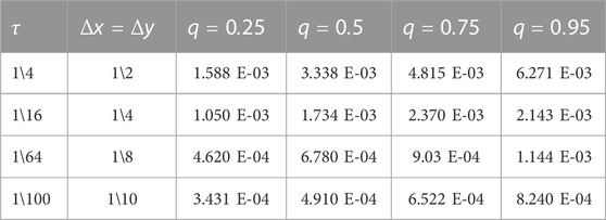
TABLE 1. Numerical results of the proposed scheme for various values of fractional order $\alpha ,$ space steps $\Delta x\text{\hspace{0.17em}and\hspace{0.17em}}\Delta y$, and time step $\Delta t$ sizes at T = 1.0.

TABLE 2

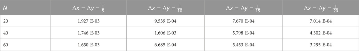
TABLE 2. Numerical results of the proposed scheme for various values of $\tau ,\Delta x,\text{and\hspace{0.17em}}\Delta y$ and a fixed value of $q=0.25.$

TABLE 3

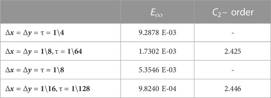
TABLE 3. Error $E_{\infty }$ and order of convergence of the IDS for the example for different values of $\tau ,\Delta x,\text{and\hspace{0.17em}}\Delta y$ and a fixed value of $q=0.5.$

FIGURE 1

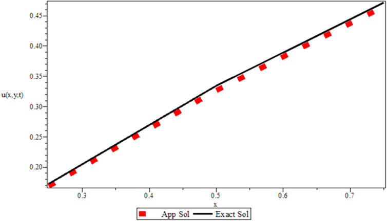
FIGURE 1. Graphical representation between the exact and approximated solutions at $q=0.35,\Delta y=0.25,N=4,\text{and\hspace{0.17em}}T=1.0$.

FIGURE 2

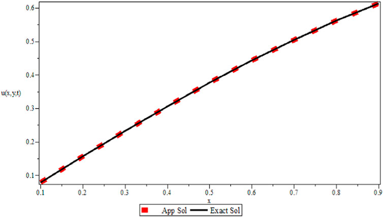
FIGURE 2. Graphical representation between the exact and approximated solutions at $q=0.35,\Delta y=0.1,N=100,\text{and\hspace{0.17em}}T=1.0.$

TABLE 4

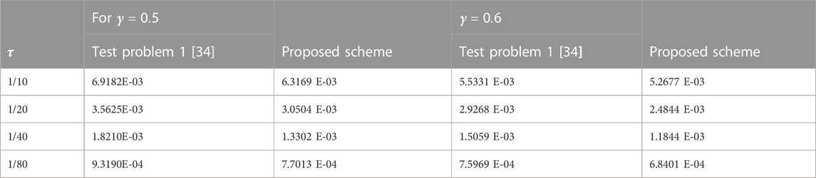
TABLE 4. Comparison between the numerical results of the proposed scheme with the previous study for various values of fractional order $\alpha$, space steps $\Delta x=\Delta y=\frac{1}{8}$, and time step $\Delta t$ sizes at T = 1.0.

FIGURE 3

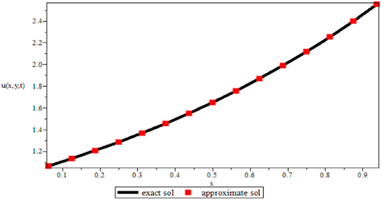
FIGURE 3. Graphical representation between the exact and approximated solutions at $q=0.5,\Delta y=0.0625,N=256,\text{and\hspace{0.17em}}T=1.0.$

8 Conclusion

A practical and quick numerical approach was designed for the FDWE. The discretization of the Riemann–Liouville integral, as described in Lemma 1, serves as the basis for the approximation. Through employing mathematical induction and demonstrating consistency and convergence, we successfully showed the theoretical analysis of stability, consistency, and convergence. The numerical results corroborated our theoretical findings and demonstrated that the suggested method is fast, convergent, and viable. This method can also be extended to different types of models arising in the realm of mathematical physics.

Data availability statement

The original contributions presented in the study are included in the article/Supplementary material; further inquiries can be directed to the corresponding authors.

Author contributions

All authors listed made a substantial, direct, and intellectual contribution to the work and approved it for publication.

Funding

The authors would like to thank the Deanship of Scientific Research at Umm Al-Qura University for supporting this work under grant code 22UQU4310396DSR68.

Acknowledgments

The authors would like to thank the referee for the valuable comments.

Conflict of interest

The authors declare that the research was conducted in the absence of any commercial or financial relationships that could be construed as a potential conflict of interest.

Publisher’s note

All claims expressed in this article are solely those of the authors and do not necessarily represent those of their affiliated organizations, or those of the publisher, the editors, and the reviewers. Any product that may be evaluated in this article, or claim that may be made by its manufacturer, is not guaranteed or endorsed by the publisher.

References

1. Ali U, 2019. Numerical solutions for two-dimensional time-fractional differential sub-diffusion equation. Ph.D., 135, pp.1–200.

Google Scholar

2. Ali U, Mastoi S, Othman WAM, Khater MM, Sohail M. Computation of traveling wave solution for nonlinear variable-order fractional model of modified equal width equation. AIMS Math (2021) 6(9):10055–69. doi:10.3934/math.2021584

CrossRef Full Text | Google Scholar

3. Khater M, Ali U, Khan MA, Mousa AA, Attia RA. A new numerical approach for solving 1D fractional diffusion-wave equation. J Funct Spaces (2021) 2021:1–7. doi:10.1155/2021/6638597

CrossRef Full Text | Google Scholar

4. Shen S, Liu F, Anh VV. The analytical solution and numerical solutions for a two-dimensional multi-term time-fractional diffusion and diffusion-wave equation. J Comput Appl Math (2019) 345:515–34. doi:10.1016/j.cam.2018.05.020

CrossRef Full Text | Google Scholar

5. Ruzhansky M, Tokmagambetov N, Torebek BT. On a non–local problem for a multi–term fractional diffusion-wave equation. Fractional Calculus Appl Anal (2020) 23(2):324–55. doi:10.1515/fca-2020-0016

CrossRef Full Text | Google Scholar

6. Yang F, Zhang Y, Li XX. Landweber iterative method for identifying the initial value problem of the time-space fractional diffusion-wave equation. Numer Algorithms (2020) 83(4):1509–30. doi:10.1007/s11075-019-00734-6

CrossRef Full Text | Google Scholar

7. Rashidinia J, Mohmedi E. Approximate solution of the multi-term time-fractional diffusion and diffusion-wave equations. Comput Appl Math (2020) 39(3):216–25. doi:10.1007/s40314-020-01241-4

CrossRef Full Text | Google Scholar

8. Feng L, Liu F, Turner I. Finite difference/finite element method for a novel 2D multi-term time-fractional mixed sub-diffusion and diffusion-wave equation on convex domains. Commun Nonlinear Sci Numer Simulation (2019) 70:354–71. doi:10.1016/j.cnsns.2018.10.016

CrossRef Full Text | Google Scholar

9. Yang JY, Zhao YM, Liu N, Bu WP, Xu TL, Tang YF. An implicit MLS meshless method for 2-D time-dependent fractional diffusion–wave equation. Appl Math Model (2015) 39(3-4):1229–40. doi:10.1016/j.apm.2014.08.005

CrossRef Full Text | Google Scholar

10. Lyu P, Liang Y, Wang Z. A fast linearized finite difference method for the nonlinear multi-term time-fractional wave equation. Appl Numer Math (2020) 151:448–71. doi:10.1016/j.apnum.2019.11.012

CrossRef Full Text | Google Scholar

11. Salehi R. A meshless point collocation method for 2-D multi-term time-fractional diffusion-wave equation. Numer Algorithms (2017) 74(4):1145–68. doi:10.1007/s11075-016-0190-z

CrossRef Full Text | Google Scholar

12. Ghafoor A, Haq S, Hussain M, Kumam P, Jan MA. Approximate solutions of time-fractional diffusion wave models. Mathematics (2019) 7(10):923. doi:10.3390/math7100923

CrossRef Full Text | Google Scholar

13. Zhuang P, Liu F. Finite difference approximation for two-dimensional time fractional diffusion equation. J Algorithms Comput Tech (2007) 1(1):1–16. doi:10.1260/174830107780122667

CrossRef Full Text | Google Scholar

14. Heydari MH, Avazzadeh Z, Yang Y. A computational method for solving variable-order fractional nonlinear diffusion-wave equation. Appl Math Comput (2019) 352:235–48. doi:10.1016/j.amc.2019.01.075

CrossRef Full Text | Google Scholar

15. Shekari Y, Tayebi A, Heydari MH. A meshfree approach for solving 2D variable-order fractional nonlinear diffusion-wave equation. Comp Methods Appl Mech Eng (2019) 350:154–68. doi:10.1016/j.cma.2019.02.035

CrossRef Full Text | Google Scholar

16. Kumar A, Bhardwaj A. A local meshless method for time fractional nonlinear diffusion wave equation. Numer Algorithms (2020) 85(4):1311–34. doi:10.1007/s11075-019-00866-9

CrossRef Full Text | Google Scholar

17. Ding H. A high-order numerical algorithm for two-dimensional time–space tempered fractional diffusion-wave equation. Appl Numer Math (2019) 135:30–46. doi:10.1016/j.apnum.2018.08.005

CrossRef Full Text | Google Scholar

18. Li M, Huang C. ADI Galerkin FEMs for the 2D nonlinear time-space fractional diffusion-wave equation. Int J Model Simulation, Scientific Comput (2017) 8(03):1750025. doi:10.1142/s1793962317500258

CrossRef Full Text | Google Scholar

19. Li L, Xu D, Luo M. Alternating direction implicit Galerkin finite element method for the two-dimensional fractional diffusion-wave equation. J Comput Phys (2013) 255:471–85. doi:10.1016/j.jcp.2013.08.031

CrossRef Full Text | Google Scholar

20. Datsko B, Podlubny I, Povstenko Y. Time-fractional diffusion-wave equation with mass absorption in a sphere under harmonic impact. Mathematics (2019) 7(5):433. doi:10.3390/math7050433

CrossRef Full Text | Google Scholar

21. Ren J, Sun ZZ. Numerical algorithm with high spatial accuracy for the fractional diffusion-wave equation with Neumann boundary conditions. J Scientific Comput (2013) 56(2):381–408. doi:10.1007/s10915-012-9681-9

CrossRef Full Text | Google Scholar

22. Yang F, Pu Q, Li XX, Li DG. The truncation regularization method for identifying the initial value on non-homogeneous time-fractional diffusion-wave equations. Mathematics (2019) 7(11):1007. doi:10.3390/math7111007

CrossRef Full Text | Google Scholar

23. Ali U, Abdullah FA. December. Modified implicit difference method for one-dimensional fractional wave equation. In: AIP conference proceedings, 2184. New York: AIP Publishing LLC (2019). No. 1.060021

Google Scholar

24. Nawaz R, Ali N, Zada L, Shah Z, Tassaddiq A, Alreshidi NA. Comparative analysis of natural transform decomposition method and new iterative method for fractional foam drainage problem and fractional order modified regularized long-wave equation. Fractals (2020) 28(07):2050124. doi:10.1142/s0218348x20501248

CrossRef Full Text | Google Scholar

25. Farid S, Nawaz R, Shah Z, Islam S, Deebani W. New iterative transform method for time and space fractional (n+1)-dimensional heat and wave type equations. Fractals (2021) 29(03):2150056. doi:10.1142/s0218348x21500560

CrossRef Full Text | Google Scholar

26. Sayevand K, Jafari H. A promising coupling of Daftardar-Jafari method and He’s fractional derivation to approximate solitary wave solution of nonlinear fractional KDV equation. Adv Math Models Appl (2022) 7(2):121–9.

Google Scholar

27. Li C, Dao X, Guo P. Fractional derivatives in complex planes. Nonlinear Anal Theor Methods Appl (2009) 71(5-6):1857–69. doi:10.1016/j.na.2009.01.021

CrossRef Full Text | Google Scholar

28. Guariglia E. Fractional calculus, zeta functions and Shannon entropy. Open Math (2021) 19(1):87–100. doi:10.1515/math-2021-0010

CrossRef Full Text | Google Scholar

29. Guariglia E. Riemann zeta fractional derivative—Functional equation and link with primes. Adv Difference Equations (2019) 2019(1):261–15. doi:10.1186/s13662-019-2202-5

CrossRef Full Text | Google Scholar

30. Ortigueira MD, Rodríguez-Germá L, Trujillo JJ. Complex grünwald–letnikov, liouville, riemann–liouville, and Caputo derivatives for analytic functions. Commun Nonlinear Sci Numer Simulation (2011) 16(11):4174–82. doi:10.1016/j.cnsns.2011.02.022

CrossRef Full Text | Google Scholar

31. Závada P. Operator of fractional derivative in the complex plane. Commun Math Phys (1998) 192:261–85. doi:10.1007/s002200050299

CrossRef Full Text | Google Scholar

32. Lin SD, Srivastava HM. Some families of the Hurwitz–Lerch Zeta functions and associated fractional derivative and other integral representations. Appl Math Comput (2004) 154(3):725–33. doi:10.1016/s0096-3003(03)00746-x

CrossRef Full Text | Google Scholar

33. Podlubny I. Geometric and physical interpretation of fractional integration and fractional differentiation (2001). arXiv preprint math/0110241.

Google Scholar

34. Zafar ZUA, Shah Z, Ali N, Kumam P, Alzahrani EO. Numerical study and stability of the Lengyel–Epstein chemical model with diffusion. Adv Difference Equations (2020) 2020:427–4. doi:10.1186/s13662-020-02877-6

CrossRef Full Text | Google Scholar

35. Sinan M, Shah K, Kumam P, Mahariq I, Ansari KJ, Ahmad Z, et al. Fractional order mathematical modeling of typhoid fever disease. Results Phys (2022) 32:105044. doi:10.1016/j.rinp.2021.105044

CrossRef Full Text | Google Scholar

36. Srivastava HM, Iqbal J, Arif M, Khan A, Gasimov YS, Chinram R. A new application of Gauss quadrature method for solving systems of nonlinear equations. Symmetry (2021) 13(3):432. doi:10.3390/sym13030432

CrossRef Full Text | Google Scholar

37. Aboud F, Jameel IT, Hasan AF, Mostafa BK, Nachaoui A. Polynomial approximation of an inverse Cauchy problem for Helmholtz-type equations. Adv Math Models Appl (2022) 7(3):306–22.

Google Scholar

38. Ali U, Khan MA, Khater M, Mousa AA, Attia RA. A new numerical approach for solving 1D fractional diffusion-wave equation. J Funct Spaces (2021) 2021:1–7. doi:10.1155/2021/6638597

CrossRef Full Text | Google Scholar

39. Ali U, Sohail M, Usman M, Abdullah FA, Khan I, Nisar KS. Fourth-order difference approximation for time-fractional modified sub-diffusion equation. Symmetry (2020) 12(5):691. doi:10.3390/sym12050691

CrossRef Full Text | Google Scholar

40. Ali U, Iqbal A, Sohail M, Abdullah FA, Khan Z. Compact implicit difference approximation for time-fractional diffusion-wave equation. Alexandria Eng J (2022) 61(5):4119–26. doi:10.1016/j.aej.2021.09.005

CrossRef Full Text | Google Scholar

41. Ganie AH, Saeed AM, Saeed S, Ali U. The Rayleigh–Stokes problem for a heated generalized second-grade fluid with fractional derivative: An implicit scheme via riemann–liouville integral. United States: Mathematical Problems in Engineering (2022).

Google Scholar

42. Tekriwal M, Duraisamy K, Jeannin JB. (2021). May. A formal proof of the Lax equivalence theorem for finite difference schemesNASA Formal Methods: 13th International Symposium, NFM 2021, Virtual Event, May 24–28, 2021, California, Cham: Springer International Publishing

Google Scholar

43. Khan MA, Ali NHM. High-order compact scheme for the two-dimensional fractional Rayleigh–Stokes problem for a heated generalized second-grade fluid. Adv Difference Equations (2020) 2020(1):233. doi:10.1186/s13662-020-02689-8

CrossRef Full Text | Google Scholar

44. Jumarie G. Modified Riemann-Liouville derivative and fractional Taylor series of non-differentiable functions further results. Comput Math Appl (2006) 51(9-10):1367–76. doi:10.1016/j.camwa.2006.02.001

CrossRef Full Text | Google Scholar

Nomenclature