Fault diagnosis of sensor pulse signals based on improved energy fluctuation index and VMD

Variational mode decomposition (VMD) has been widely applied in sensors. However, the mode number and balance parameter seriously limit VMD application. To solve this problem, this study proposes a novel method, which combines an improved energy fluctuation index (IEFI) and modified VMD (MVMD). In the proposed method, IEFI provided better performance to resist interference from random impulses by considering the periodicity of fault feature components. Consequently, it is applied to determine the initial center frequency for MVMD, which fixed the problem of the mode number. Moreover, a novel balance parameter search strategy, which can adaptively determine the optimal balance parameter, is combined with MVMD whose stop condition is replaced by kurtosis to extract the fault feature. Simulation results indicated that the proposed method does well in detecting the feature of a periodic impulse signal from the signal polluted by some interference impulses. Moreover, the bearing fault diagnosis results demonstrate that the proposed method can accurately detect bearing fault features. Furthermore, the method was validated with bearing fault data. The results showed that the method can accurately extract the fault characteristics of the impulse signal and achieve fault diagnosis.

1 Introduction

Industrial equipment and systems have been increasingly moving toward larger, more complex, and integrated features, which lead to increased uncertainty in the system operation. To ensure the safe operation of equipment, extracting fault characteristics from signals collected by the sensors is necessary to achieve the purpose of fault diagnosis [1]. Sensors collect a large amount of image [2, 3] and data information [4–8], based on which many functions can be implemented.

Recent studies show the effectiveness of vibration signals in fault diagnosis [9]. Meanwhile, the fault response of the bearing and gearbox serves as an impact component in the vibration signal [10]. Unfortunately, the impulse response from the early fault is often submerged by noise from other running components and environments because the impulse response is too weak. Thus, an effective impulse signal detection method is necessary to evaluate the operating status of the rotation machine. Envelope analysis can effectively detect impulse signals but is ineffective in low signal-to-noise ratio (SNR) data. WT works well in heavy noisy signals but is seriously limited by basic functions [11]. EMD and EEMD can adaptively decompose complex signals into server modals but lack the rigorous mathematical theory. Fortunately, variational mode decomposition (VMD) can decompose low SNR signals into server modes under the number of suitable modes and the balance parameter [12]. Meanwhile, Wang et al. [13] investigated the filter property of VMD by simulation signals and found that VMD can be implemented to detect impulse signals. Additionally, Wang et al. [14] applied VMD to detect impulse components in the signal from a rotor system. The results indicate that VMD works better than EMD and EEMC. Li et al. [15] analyzed the signal from a wind turbine by combining VMD and blind-source separation to detect the bearing crack fault. Li et al. [16] introduced VMD to calculate the central frequency and combined it with data-driven time–frequency analysis to diagnose the gear fault. Diagnosing faults by VMD provides advantages to identify different health conditions [17].

Based on the aforementioned description, VMD has been widely applied in the fault detection field. However, the mode number and balance parameter are determined based on the experience in the aforementioned articles. To solve this problem, many researchers paid attention to determining the mode number and balance parameter, and some results can be summarized as follows: first, research combined VMD with some intelligent search algorithms, such as grasshopper optimization algorithm, salp swarm algorithm, and particle swarm optimization [18–21]. By using intelligent search algorithms, the mode number and balance parameter can be determined adaptively and effectively. However, accepting the computational efficiency is difficult. Second, research studies put forward some other methods whose mode number is based on the fast Fourier transformation (FFT) spectrum of the decomposition result, such as independence-oriented VMD, adaptive VMD, and detrended fluctuation analysis VMD (DFA-VMD) [22–24]. These methods can adaptively select system parameters. However, some parameters must be determined artificially, and the over-decomposition phenomenon frequently occurs in these methods. Meanwhile, some researchers used iteration methods to search system parameters for VMD. Such methods include coarse-to-fine VMD and tentative VMD, which are often designed in two stages, to determine the target sub-mode and refine the sub-mode to enhance the impulse component. Finally, the initial center frequency-guided VMD (ICF-VMD) method is proposed in Refs. 25–Refs. 28. Compared with other adaptive VMD methods, ICF-VMD works well to extract bearing fault features and has better computational efficiency [29]. ICF-VMD is also designed in two stages: to determine the center frequency by the energy fluctuation variance and to refine the balance parameter to enhance the fault feature. However, the energy fluctuation variance is sensitive to the random impulse, and the balance parameter search process is limited in a narrow range. Two drawbacks may explain the failure of extracting the bearing fault feature.

To solve the aforementioned problems and improve the computational efficiency, this study proposes a novel method which combines an improved energy fluctuation index (IEFI) and modified VMD (MVMD). IEFI, a method based on the original energy fluctuation index and the subscript’s variance of the energy whose value is greater than the mean, is used to determine the center frequency for MVMD. Consequently, the mode number can be fixed as one, and the balance parameter is the only parameter that needs to be determined. In this research study, a novel balance parameter search strategy from MVMD was used to extract the bearing fault feature. The initial balance parameter is determined based on the center frequency from the IEFI, which enhances the adaptability of the search strategy. The MVMD, whose stop condition is replaced by kurtosis, has good computational efficiency. In summary, IEFI ensures that the proposed method works well to process the signal, which includes some random impulses. The novel search strategy and MVMD ensure the computational efficiency of the proposed method. The effectiveness of the proposed method is examined by the simulation and experiment signals. The advantages of the proposed method are highlighted by comparing it with some existing methods.

The rest of the paper is organized as follows. Section 2 describes the proposed method. Section 3 organizes the results of the numerical experiment, case study, and comparison. Section 4 presents a concise summary.

2 The proposed method

This section introduces the basic theory about the IEFI and the MVMD to help in understanding the proposed method.

2.1 Modified VMD

VMD decomposes signals into a series of sub-modes through some Wiener filter banks. Its model is described as follows:

$\begin{array}{l}\begin{array}{l}\min \\ \left\{{\mathrm{u}}_{\mathrm{k}}\right\},\left\{{\omega }_{\mathrm{k}}\right\}\end{array}\left\{{\displaystyle \sum }_{k=1}^K{‖{\partial }_t\left[\left(\delta \left(\mathrm{t}\right)+\frac{j}{\pi t}\right)*u_k\left(\mathrm{t}\right)\right]{e^{-j{\omega }_k}}^t‖}_2^2\right\}\\ s.t.{\displaystyle \sum }_{k=1}^K{u}_k\left(\mathrm{t}\right)=f\end{array},(1)$

where $u_k$ and ${\omega }_k$ denote the sub-mode and its center frequency, respectively. By introducing Lagrangian multipliers and penalty technology, Eq. 1 can be written as follows:

$\begin{array}{l}L\left(\left\{{\mathrm{u}}_{\mathrm{k}}\right\},\left\{{\omega }_{\mathrm{k}}\right\},\lambda \right)=\alpha {\displaystyle \sum }_{k=1}^K{‖{\partial }_t\left[\left(\delta \left(\mathrm{t}\right)+\frac{j}{\pi t}\right)*u_k\left(\mathrm{t}\right)\right]{e^{-j{\omega }_k}}^t‖}_2^2+\\ {‖f\left(\mathrm{t}\right)-{\displaystyle \sum }_{k=1}^K{u}_k\left(\mathrm{t}\right)‖}_2^2+〈\lambda \left(\mathrm{t}\right),f\left(\mathrm{t}\right)-{\displaystyle \sum }_{k=1}^K{u}_k\left(\mathrm{t}\right)〉\end{array},(2)$

where $\alpha$ is the balance parameter, and $\lambda \left(t\right)$ means the Lagrangian multiplier parameter. Equation 2 can be solved through an alternate direction method of multiplier (ADMM) technology, and its process is described in.

Algorithm 1: ADMM for VMDInitialize: ${\mathrm{u}}_{\mathrm{k}},{\omega }_{\mathrm{k}},\lambda ,n\leftarrow 1$

$\mathbf{U}\mathbf{p}\mathbf{d}\mathbf{a}\mathbf{t}\mathbf{e}{u}_k:{\widehat{u}}_k^{n+1}\left(\omega \right)\leftarrow \frac{\widehat{f}\left(\omega \right)-{\sum }_{i\ne k}{\widehat{u}}_k^{n+1}\left(\omega \right)+\frac{{\widehat{\lambda }}^n\left(\omega \right)}{2}}{1+2\alpha {\left(\omega -{\omega }_k^n\right)}^2},(3)$

$\mathbf{U}\mathbf{p}\mathbf{d}\mathbf{a}\mathbf{t}\mathbf{e}{\omega }_k:{\omega }_k^{n+1}\leftarrow \frac{{\int }_0^{\infty }\omega {\left|u_k^{n+1}\left(\omega \right)\right|}^{2}d\omega }{{\int }_0^{\infty }{\left|u_k^{n+1}\left(\omega \right)\right|}^{2}d\omega },(4)$

$\mathbf{U}\mathbf{p}\mathbf{d}\mathbf{a}\mathbf{t}\mathbf{e}\lambda :{\lambda }^{n+1}\left(\omega \right)\leftarrow {\lambda }^n\left(\omega \right)+\tau \left(f\left(\omega \right)-{\displaystyle \sum }_k{u}_k^{n+1}\left(\omega \right)\right).(5)$

Convergence condition: ${{\sum }_{\mathrm{k}}‖{\widehat{\mathrm{u}}}_{\mathrm{k}}^{\mathrm{n}+1}-{\widehat{\mathrm{u}}}_{\mathrm{k}}^{\mathrm{n}}‖}_2^2/{‖{\mathrm{u}}_{\mathrm{k}}^{\mathrm{n}+1}‖}_2^2<\epsilon$

According to, $\tau$ denotes the learning rate, which can be fixed as zero when VMD is applied to denoise the sub-components instead of recovering them. Understanding the mode number and the balance parameter is easy and important in VMD. According to Ref. 12, the mode number can be fixed as one with the help of the right center frequency. On the other hand, according to Ref. 30, this method is applied to detect bearing fault features. Thus, the mode number is set as one. This study applies envelope analysis to process the signal filtered by VMD. Consequently, VMD is assumed to be the filter in this study, and the learning rate $\tau$ should be 0 based on 11. Given that the purpose of VMD in this study is not to recover sub-components, its convergence condition can be modified to obtain a higher computational efficiency. Kurtosis is widely applied as index for diagnosing bearing fault, and it will be applied to construct a new convergence condition for VMD in this study. The new convergence condition is defined as follows:

$\mathrm{k}\mathrm{u}\mathrm{r}\left(u^n\right)/\mathrm{k}\mathrm{u}\mathrm{r}\left(u^{n+1}\right)>\eta ,(6)$

in which, $\text{kur}\left(·\right)$ denotes the kurtosis operator and $\eta$ is set as 0.99, which can ensure that the kurtoses of the two adjacent generations have the same level. VMD, which is based on this convergence condition, is named MVMD in this study. By modifying the convergence condition as Eq. 6, MVMD not only has a good performance in extracting bearing fault features but also has higher computational efficiency, which is friendly with engineering applications.

2.2 Improved energy fluctuation index

Based on 11, Refs. 28, the number of modes can be set as one with the help of a correct center frequency. According to Ref. 28, the center frequency is determined based on the variance of energy fluctuations whose mathematical formula can be written as:

$A\left(f_j\right)=\sqrt{{\displaystyle \sum }_{i=1}^N{\left(TF\left(t_i,f_j\right),-\overline{TF\left(t_i,f_j\right)}\right)}^2,}(7)$

where $TF\left(t,j\right)$ is the time–frequency analysis result. In this research, it is calculated by the short-time Fourier transform (STFT), which is shown as follows:

$TF\left(t,f\right)={\int }_{-\infty }^{+\infty }x\left(\tau \right)w\left(t-\tau \right)e^{-2\mathrm{j}\pi \mathrm{f}\tau }d\tau .(8)$

However, the variance of energy fluctuation is weak to resist the interferences from the random impulses and neglects the period property of the real fault response. To fill these gaps, an IEFI is proposed to determine the center frequency. The new index is defined as:

$IEF\left(f_j\right)=A\left(f_j\right)\times \exp \left\{-\text{var}\left(S_{\mathrm{S}}\left(f_j\right)-S_{\mathrm{F}}\left(f_j\right)\right)\right\}.(9)$

$S_{\mathrm{S}}\left(f_j\right)$ corresponds to the subscripts of the elements from the second to the last, whereas $S_{\mathrm{F}}\left(f_j\right)$ corresponds to the subscripts of the elements from the first to the last but one. For the periodic impulses, all of the elements in $\left[S_S\left(f_j\right)-S_{\mathrm{F}}\left(f_j\right)\right]$ should be constant. Thus, their variance should be equal to zero. Therefore, the exponent term shown in Eq. 9 will be close to one for periodic impulses. However, for aperiodic impulses and noise, the distribution of the elements in $\left[S_S\left(f_j\right)-S_{\mathrm{F}}\left(f_j\right)\right]$ is irregular. Thus, their variance is far from zero, which will weaken the exponent term shown in Eq. 9. Based on the aforementioned description, implementing IEFI to identify periodic impulses is more accurate than implementing raw energy fluctuations.

2.3 The proposed method

The center frequency can be obtained from the IEFI, and the number of modes is set as one based on it. To run VMD successfully, the balance parameter should be determined first. Generally, the intelligent search algorithm and iterative search process are applied to solve this problem. However, accepting the computational efficiency of intelligent search algorithm is difficult. Thus, this study proposes a novel iterative search strategy to determine the balance parameter. The novel method is named IEFI–MVMD, which combines the improved energy fluctuation index and the modified VMD. The main steps of IEFI–MVMD are given as follows:

Step 1:. The signal is processed by STFT with a window length of 512 and an overlap of 256.

Step 2:. The IEFI is applied to evaluate the periodic impulse for each frequency. Additionally, the center frequency is the one with the largest IEFI.

Step 3:. The balance parameter is initialized on the basis of

$\alpha ={\phi /\min \left(0.5-{\omega }_k,{\omega }_k\right)}^2,(10)$

where $\phi$ is defined as five based on Eq. 3. From Eq. 3, one can easily understand that $\phi =5$ ensures the frequency response factor of the frequency boundary is not over 1/10.

Step 4:. The raw signal is processed by using the MVMD method whose modes’ number is fixed as one, and the kurtosis of the decomposition result is marked as $K_1$.

Step 5:. The balance parameter is replaced by $\delta \times \alpha$, and $\delta$ is fixed as 1.5 in this study. The kurtosis of the new result is calculated and marked as $K_2$. If $K_1$ is less than $K_2$, then, Steps 4 and 5 are repeated until $K_1$ is larger than $K_2$.

Step 6:. The final result (corresponding to $K_1$) is processed through envelope demodulation technology to obtain the squared envelope spectrum, which can clearly show the fault feature frequency.To understand the IEFI–MVMD clearly, Figure 1 displays the corresponding flowchart.

FIGURE 1

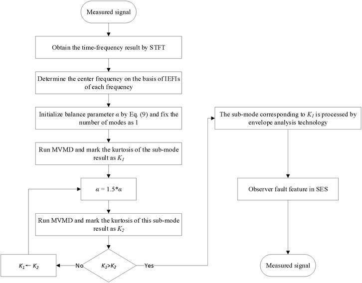
FIGURE 1. Flowchart of IEFI–MVMD

3 Case study

To examine the effectiveness of the proposed method, this section introduces a simulation signal and two bearing fault signals. Meanwhile, the superiority of the proposed method is highlighted by comparing it with some existing methods.

3.1 Simulation

The simulation signal includes the harmonic component ($y_1$), the periodic impulse ($y_2$), the aperiodic impulse ($y_3$), and the Gaussian noise ($n\left(t\right)$). The simulation signal can be written as follows:

$y\left(t\right)=y_1\left(t\right)+y_2\left(t\right)+y_3\left(t\right)+n\left(t\right),(11)$

$y_1\left(t\right)=A\times \sin \left(2\pi \times 200t\right),(12)$

$y_2\left(t\right)=2\times e^{0.1\times 2\pi \times 2000t}\sin \left(2\pi \times 2000t\times \sqrt{1-0.1^2}\right),(13)$

$y_3\left(t\right)=3\times e^{0.1\times 2\pi \times 1200t}\sin \left(2\pi \times 1200t\times \sqrt{1-0.1^2}\right).(14)$

In the simulation signal, the frequency of the impulse signal is set at $f_i=40\text{Hz}$. The sampling frequency is 20 kHz, and the length of the simulation signal is 10 k points. The density of Gaussian noise is 0.4. The simulation signal is illustrated in Figure 2. From Figure 2D, the periodic impulses can be seen as seriously polluted by the noise. Even in its squared envelope spectrum (SES) shown in Figure 3, observing the features of the periodic impulses is difficult.

FIGURE 2

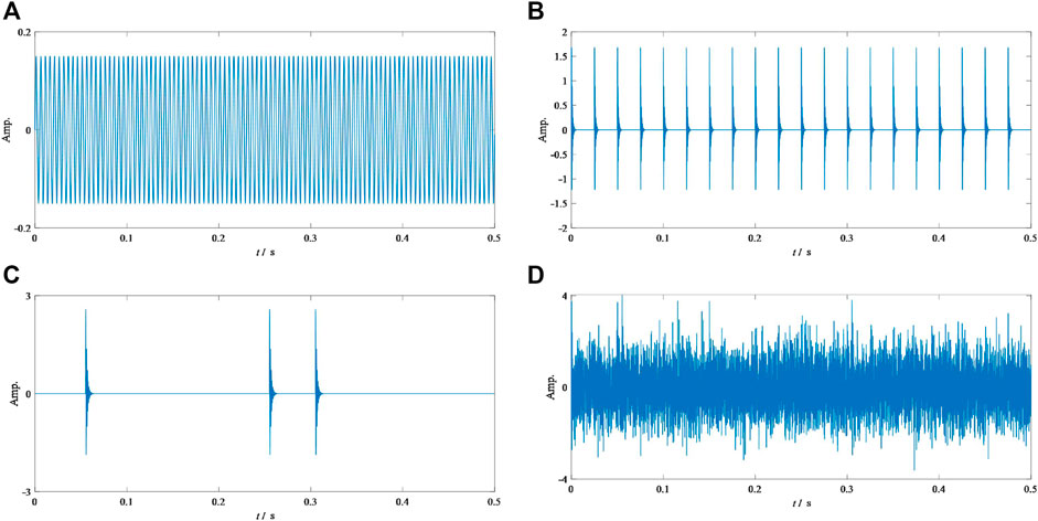
FIGURE 2. Simulation signal: (A) harmonic component $y_1$, (B) periodic impulse component $y_2$, (C) interface impulse component $y_3$, and (D) composite signal $y$.

FIGURE 3

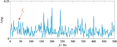
FIGURE 3. SES of the simulation signal.

Then, the proposed method is applied to analyze this signal. To begin with, the signal is analyzed by the IEFI, and Figure 4 shows the results. As shown in Figure 4A, three interference impulses occur in the simulation signal, which is consistent with the results shown in Figure 2C. Figure 4B shows the result above IEFI. Additionally, the frequency corresponding to the largest IEFI is 1,992 Hz, which is close to the design frequency in Eq. 13. Then, the balance parameter is determined by Eq. 9. Figure 4C is the time domain waveform (TDW) of the results. Compared to the raw TDW shown in Figure 2D, some periodic impulses are clearly shown in this figure. Importantly, the fundamental feature frequency and its harmonics are clearly displayed in its SES, as shown in Figure 4D. Consequently, our method succeeds in detecting the feature of the periodic impulses from the signal polluted by some interference impulses.

FIGURE 4

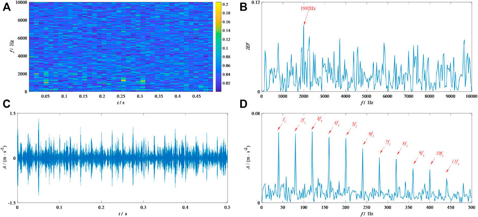
FIGURE 4. Results by the IEFI–MVMD of the simulation signal: (A) STFT, (B) IEFI, (C) TDW, and (D) SES.

3.2 Case I

This section describes the implementation of the proposed method to analyze some signals from the bearing fault experiment. The signals used in this section come from the Society for Machinery Failure Prevention Technology (MFPT). According to description in MFPT, the tested bearing’s faults include healthy conditions, outer race fault conditions, and inner race fault conditions. Figure 5 illustrates the TDW and the corresponding SES of these signals used in this section. From Figure 4, the amplitudes of the fault feature frequencies of the healthy bearing can be described as extremely low. Figures 5C,D show the signal of the inner race fault bearing. Moreover, some periodic impulses can be easily found in Figure 5C. Moreover, some information about the inner race fault can be easily found in its SES as shown in Figure 5D, but some interferences occur in it. Figures 5E, F show the information about the signal of the outer race fault. Unfortunately, it is difficult to find the periodic impulses. Nonetheless, the 1xBPFO and 2x can be clearly observed in it.

FIGURE 5

FIGURE 5. Signals from MFPT: (A) and (B) correspond to the TDW and SES of the healthy bearing, (C) and (D) correspond to the TDW and SES of the inner race fault bearing, and (E) and (F) correspond to the TDW and SES of the outer race fault bearing.

Finally, this study calculates the ratio of the amplitudes between the interference frequency (IF) and fundamental feature frequency to show the superiority of the proposed method conveniently. A large value of the ratio means a good result for extracting fault features. We applied this ratio in the results of the inner race fault signal.

First of all, IEFI–MVMD is applied to process these signals. Figure 6 shows the results about the IEFI, whereas Figure 6 presents the results of the proposed method. According to Figure 5, the initial center frequencies for the healthy bearing, the inner fault bearing, and outer fault bearing should be 6,103, 3,051, and 1,907 Hz, respectively. From Figure 7B, the amplitude for either BPFO or BPFI is low, which means the bearing is healthy. The results of the healthy bearing indicate that our method can accurately deal with these kinds of signals. Figure 7D shows the SES of the results by IEFI–MVMD for the inner race fault bearing signal. Carefully comparing it with Figure 4D, the ratio shown in Figure 7D is 1.14, which is larger than the ratio shown in Figure 4D. This finding means that IEFI–MVMD enhances the inner race fault feature. Figure 7F illustrates the SES of the results by IEFI–MVMD for the outer race fault bearing signal. Comparing it to Figure 4C, the fault feature is enhanced by IEFI–MVMD efficiency because the high-order harmonics (3x, 4x, and 5x) can only be found in Figure 6F. Based on the aforementioned description, our method can be said to reflect the real health status, including the health, inner race fault, and outer race fault.

FIGURE 6

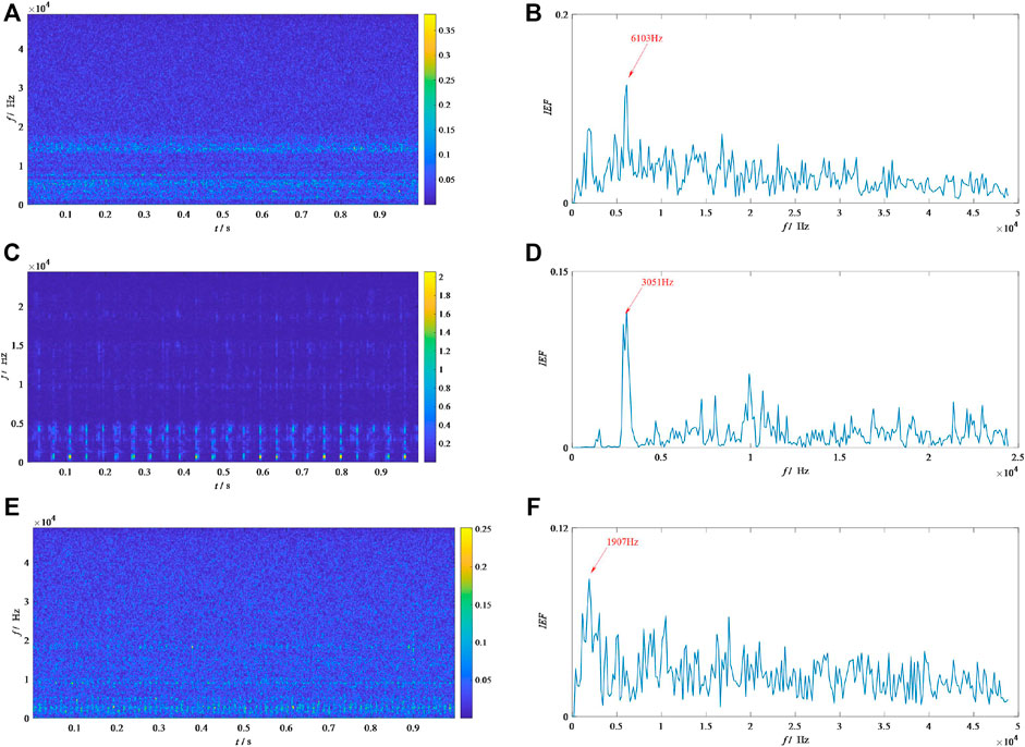
FIGURE 6. Results of IEFI for signals from MFPT: (A) and (B) correspond to the STFT and IEFI of the healthy bearing, (C) and (D) correspond to the STFT and IEFI of the inner race fault bearing, and (E) and (F) correspond to the STFT and IEFI of the outer race fault bearing.

FIGURE 7

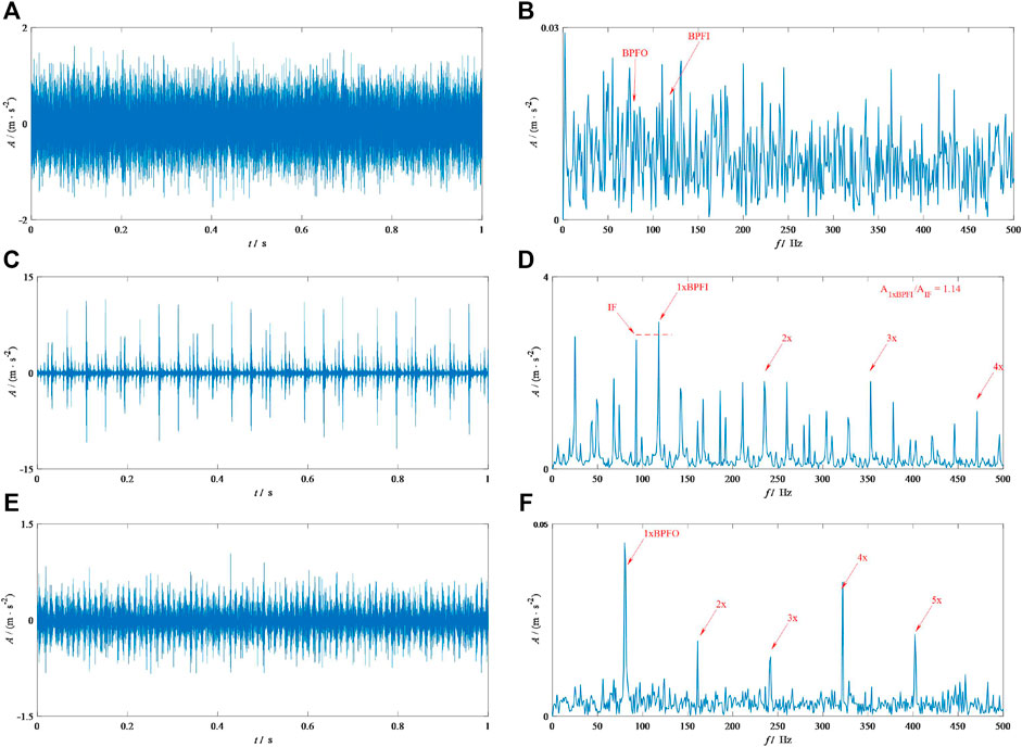
FIGURE 7. Final results of the IEFI–MVMD for signals from MFPT: (A) and (B) correspond to the TDW and SES of the healthy bearing, (C) and (D) correspond to the TDW and SES of the inner race fault bearing, and (E) and (F) correspond to the TDW and SES of the outer race fault bearing.

The signals of inner and outer race fault bearings are analyzed by some other methods, including the fast kurtogram (FK), the ICF-VMD, and a new method that combines the IEFI and the raw VMD. For convenience, this method is named IEFI–VMD.

Figure 8 shows the results from FK. From Figure 8A, the optimal demodulation frequency band (ODFB) by FK for MFPT-I is in level 1 with the center frequency 6,103 Hz. In addition, Figure 8B shows the SES of the signal based on this ODFB. From Figure 9B, the fault features including 1 x BPFI, 2x, and 3x are clearly shown. However, the ratio shown in its upward right corner is lower than the result shown in Figure 7D, which means that our method works better than FK to extract the inner fault features. Moreover, Figure 8C shows that the ODFB by FK for MFPT-O is located in level 6 with the center frequency 17,929 Hz. In addition, Figure 8D illustrates the SES of the signal based on this ODFB. By comparing Figure 8D with Figure 5F, the high-order harmonics (4x and 5x) can only be easily found in Figure 8F. Thus, FK cannot catch up with the level of our method in dealing with both the inner and outer race fault signals.

FIGURE 8

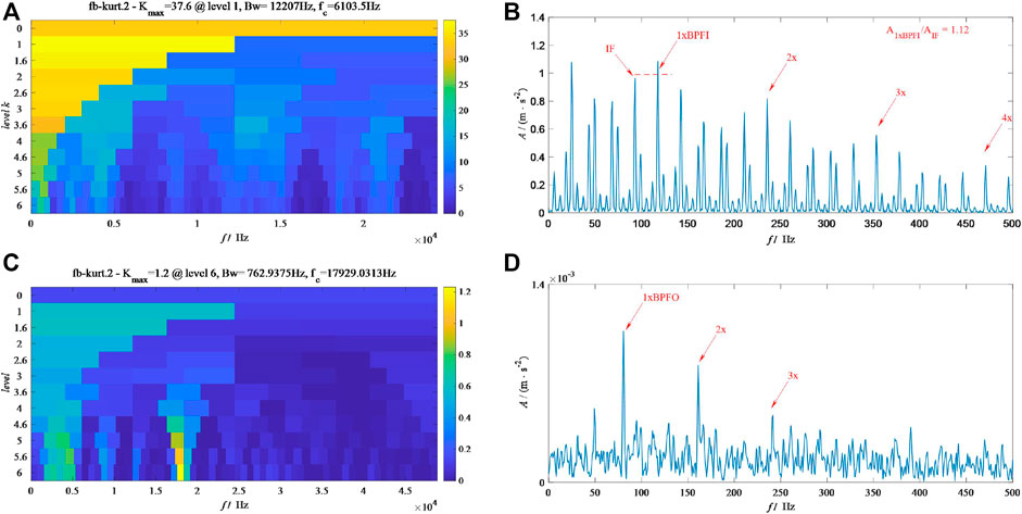
FIGURE 8. Results from FK for the MFPT signals: (A) and (B) correspond to the kurtogram and the corresponding SES of the inner race fault bearing; (C) and (D) correspond to the kurtogram and the corresponding SES of the outer race fault bearing.

FIGURE 9

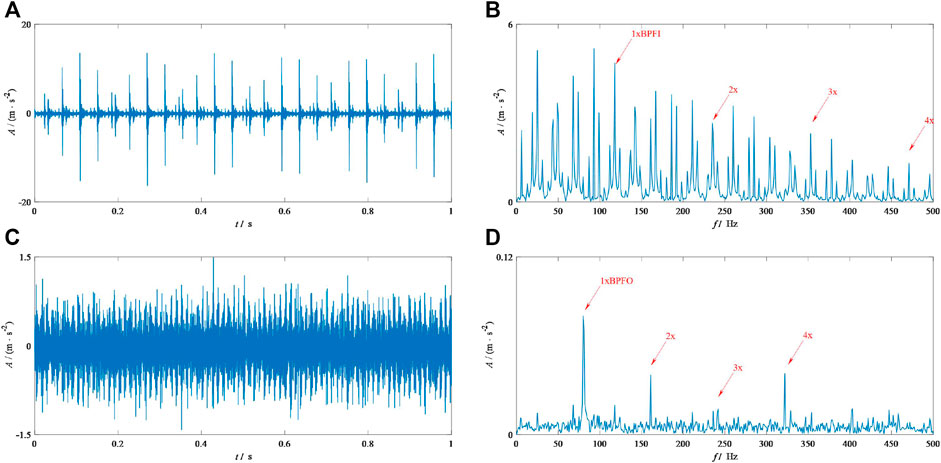
FIGURE 9. Results from ICF-VMD for the MFPT signals: (A) and (B) correspond to the TDW and the corresponding SES of the inner race fault bearing; (C) and (D) correspond to the TDW and the corresponding SES of the outer race fault bearing.

Figure 9 and Figure 10 show the results from ICF-VMD and IEFI–VMD, respectively. Figure 9A shows the TDW of the results by ICF-VMD for MFPT-I, and Figure 9B shows its SES. By comparing Figures 8B, 6D, using the proposed method to diagnose faults provides better performance than using ICF-VMD because the amplitude of 1xBPFI is not the highest in SES and other interferences exist in it. Figure 9B displays the TDW of the results by ICF-VMD for MFPT-O, and Figure 9D shows the corresponding SES. By comparing Figures 9D, 7F, determining that the high-order fault features (3x and 5x) are weaker than the results is not difficult, as shown in Figure 7D. Figure 10A shows the TDW of the results by IEFI–VMD for MFPT-I, and Figure 10B shows its corresponding SES. By comparing Figures 10B, 7D, determining the differences between them is difficult. The ratio shown in the upward right corner of Figure 10B tells us that our method has a slight lead. Figure 10C shows TDW of the result by IEFI–VMD for MFPT-O, and Figure 10D shows its SES. From Figure 10D, some interference occurs near the fault feature 3x. Nonetheless, in Figure 7F, it is shown clearly. This finding means that the proposed method has a slight lead. More importantly, the computation efficiencies of IEFI–MVMD and IEFI–VMD are highly different, and we will show it toward the end of this paper to highlight the superiority of our introduced method.

FIGURE 10

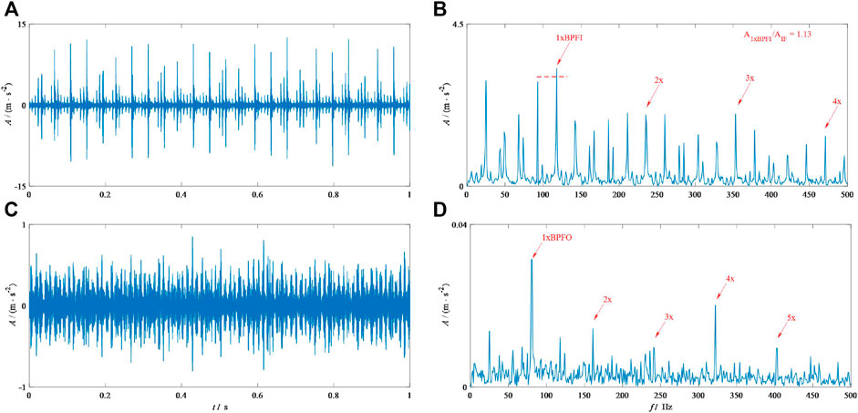
FIGURE 10. Results from IEFI–VMD for the MFPT signals: (A) and (B) correspond to the TDW and the corresponding SES of the inner race fault bearing; (C) and (D) correspond to the TDW and the corresponding SES of the outer race fault bearing.

3.2 Case II

This section applies the introduced method to analyze another fault bearing signal, which includes some interference impulses. This kind of signal effectively highlights the advantage of our method.

The signal comes from Curtin University. The type of the test bearing is MB ER-16K, and a local defect exists in its outer race. For a convenient description, this signal is marked as CU-O in this research study. The shaft speed is 1,740 rpm, and the BPFO is 103.6 Hz from Ref. 31. The sampling frequency is 51.2 kHz, and the length of the signal applied in this study is 1 s.

Figure 11 shows the TDW and its SES. From Figure 11A, some certain interference impulses (marked by red point) exist in the measured signal. In Figure 11B, determining the fault feature frequency and its harmonics is difficult due to the interference from noise. Then, our method is applied to analyze this signal, and Figure 12 shows the results. From Figure 12A, the center frequency of the interference impulses is near 10 kHz. However, the result of IEFI shown in Figure 12B tells us that the center frequency of the periodic impulses should be 3,100 Hz, and the value of the interference impulses is extremely low. This result means that IEFI can effectively suppress the interference impulses. Figure 12C shows the TDW of the result by our method for CU-O. According to Figure 12C, some periodic impulses are clearly shown and the interference impulses are suppressed effectively. Figure 12D shows its SES. The fault features including 1xBFO, 2x, 3x, and 4x are clearly shown in it. Consequently, our method can be said to have succeeded in detecting the bearing fault feature accurately and is strong enough to resist the interference from the aperiodic impulses.

FIGURE 11

FIGURE 11. Raw signals from CU-O: (A) TDW and (B) SES.

FIGURE 12

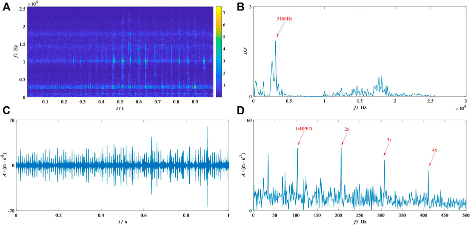
FIGURE 12. Results from IEFI–MVMD: (A) STFT, B) IEFI, (C) TDW, and (D) SES.

Signal CU-O is also processed by FK, ICF-VMD, and IEFI–VMD. In addition, Figure 13 and Figure 14 show their results, respectively. From Figure 13A, the ODFB FK can be seen at level 4.5 with the center frequency of 9,066 Hz. Additionally, according to SES from Figure 13B, only the fundamental fault feature frequency can be observed easily. Evidently, a large gap exists between Figures 13B, 12D. Figure 14C shows the TDW by ICD-VMD. According to Figure 14C, some interference impulses remain included in the filtered signal. Moreover, based on its SES shown in Figure 14D, observing the fundamental fault feature frequency and its harmonics is difficult due to the existence of noise and interference impulses. Figure 14C shows the TDW by IEFI–VMD for signal CU-O, and Figure 14D shows its SES. From Figure 14C, determining that the interference impulses are suppressed effectively is easy. Subsequently, according to SES from Figure 14D, the fundamental fault feature frequency and its harmonics can be observed clearly. By comparing it with the result shown in Figure 13D, we think they have the same level. However, the computational efficiency of IEFI–VMD is much farther from IEFI–MVMD.

FIGURE 13

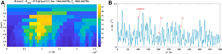
FIGURE 13. Results from FK for signal CU-O: (A) kurtogram and (B) SES.

FIGURE 14

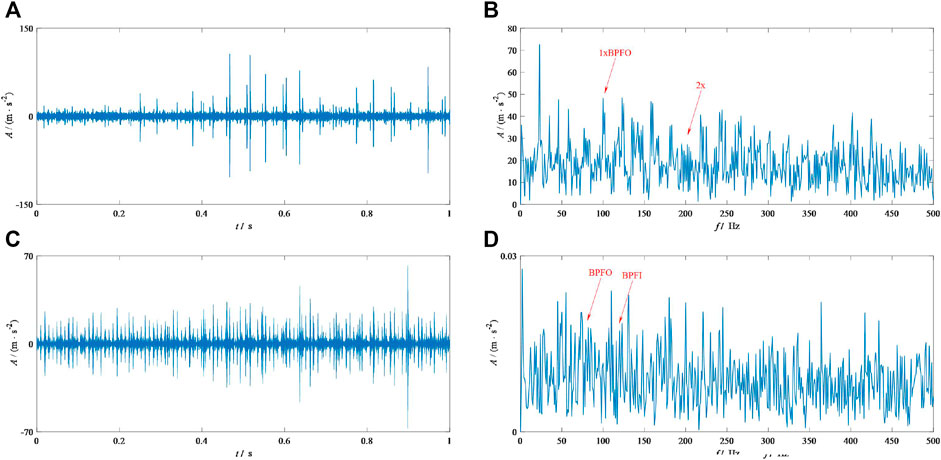
FIGURE 14. Results from signal CU-O: (A)ICF-VMD TDW, (B) ICF-VMD SES, (C) IEFI–VMD TDW, and (D) IEFI–VMD SES.

To obtain the calculation time of IEFI–MVMD, IEFI–VMD, and ICF-VMD accurately, each method is tested three times in the same computer whose hardware is Intel(R) Core (TM) i7-9700 CPU @ 3.00 GHz 3.00 GHz. The mean is applied to evaluate the computational efficiency. Table 1 shows the results. From this table, the calculation time of our method is the lowest for each signal, which means our method has the highest computational efficiency among the three methods. Consequently, IEFI–MVMD can detect the bearing fault feature with great computational efficiency.

TABLE 1

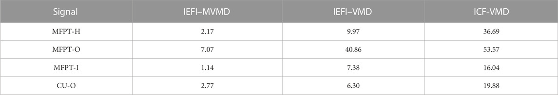
TABLE 1. Calculation time for each signal unit: (s).

4 Conclusion

This study proposes a novel method named IEFI–MVMD to detect the fault feature of the bearing. IEFI–MVMD has a strong power to resist interference from aperiodic impulses and has high computational efficiency. Specifically, the guide-center frequency is determined by the IEFI calculated based on the subscript of the elements. If it is greater than the mean, the ability to resist random impulses could be enhanced. The fault feature is extracted by the MVMD whose convergence condition is built up by decomposing kurtosis, which ensures that the proposed method has high computational efficiency. The proposed method succeeds in analyzing signals from inner and outer race fault bearings and healthy bearings. The advancement of the proposed method is highlighted by comparing it to other existing methods.

Data availability statement

Publicly available datasets were analyzed in this study. These data can be found here: https://www.mfpt.org/fault-data-sets/.

Author contributions

Funding acquisition: YL and YM; project administration: YL and YM; conceptualization: YL and XC; validation: YL and YC; formal analysis: YL and XC; investigation: YL and XC; data curation: YL and XC; writing—original draft preparation: YL; and writing—review and editing: YL. All authors have read and agreed to the published version of the manuscript.

Funding

This work was supported by the National Natural Science Foundation of China (Grant No. U2034209), the Postdoctoral Science Foundation of China (Grant No. 2021M700590), and the Fundamental Research Funds for the Central Universities (Grant No. 2022CDJJMRH-008).

Acknowledgments

The authors would like to thank all the people who participated in the studies.

Conflict of interest

The authors declare that the research was conducted in the absence of any commercial or financial relationships that could be construed as a potential conflict of interest.

Publisher’s note

All claims expressed in this article are solely those of the authors and do not necessarily represent those of their affiliated organizations, or those of the publisher, the editors, and the reviewers. Any product that may be evaluated in this article, or claim that may be made by its manufacturer, is not guaranteed or endorsed by the publisher.

References

1. He B, Huang Y, Wang D, Yan B, Dong D. A parameter-adaptive stochastic resonance based on whale optimization algorithm for weak signal detection for rotating machinery. Measurement (2019) 136:658–67. doi:10.1016/j.measurement.2019.01.017

CrossRef Full Text | Google Scholar

2. Zhu Z, He X, Qi G, Li Y, Cong B, Liu Y. Brain tumor segmentation based on the fusion of deep semantics and edge information in multimodal MRI. Inf Fusion (2023) 91:376–87. doi:10.1016/j.inffus.2022.10.022

CrossRef Full Text | Google Scholar

3. Wang Y, Qi G, Li S, Chai Y, Li H. Body part-level domain alignment for domain-adaptive person re-identification with transformer framework. IEEE Trans Inf Forensics Security (2022) 17:3321–34. doi:10.1109/tifs.2022.3207893

CrossRef Full Text | Google Scholar

4. Fan L, Chai Y, Chen X. Trend attention fully convolutional network for remaining useful life estimation. Reliability Eng Syst Saf (2022) 225:108590. doi:10.1016/j.ress.2022.108590

CrossRef Full Text | Google Scholar

5. Liu B, Chai Y, Liu Y, Huang C, Wang Y, Tang Q. Industrial process fault detection based on deep highly-sensitive feature capture. J Process Control (2021) 102:54–65. doi:10.1016/j.jprocont.2021.04.003

CrossRef Full Text | Google Scholar

6. Liu B, Chai Y, Huang C, Fang X, Tang Q, Wang Y. Industrial process monitoring based on optimal active relative entropy components. Measurement (2022) 197:111160. doi:10.1016/j.measurement.2022.111160

CrossRef Full Text | Google Scholar

7. Liu B, Chai Y, Jiang Y, Wang Y. Industrial Fault detection based on discriminant enhanced stacking auto-encoder model. Electronics (2022) 11(23):3993. doi:10.3390/electronics11233993

CrossRef Full Text | Google Scholar

8. Zhu Z, Lei Y, Qi G, Chai Y, Mazur N, An Y, et al. A review of the application of deep learning in intelligent fault diagnosis of rotating machinery. Measurement (2022) 206:112346. doi:10.1016/j.measurement.2022.112346

CrossRef Full Text | Google Scholar

9. Yu J, Hu T, Liu H. A new morphological filter for fault feature extraction of vibration signals. IEEE Access (2019) 7:53743–53. doi:10.1109/access.2019.2912898

CrossRef Full Text | Google Scholar

10. Zhang H, He Q. Tacholess bearing fault detection based on adaptive impulse extraction in the time domain under fluctuant speed. Meas Sci Tech (2020) 31(7):074004. doi:10.1088/1361-6501/ab7dec

CrossRef Full Text | Google Scholar

11. Yan R, Gao RX, Chen X. Wavelets for fault diagnosis of rotary machines: A review with applications. Signal Processing (2014) 96:1–15. doi:10.1016/j.sigpro.2013.04.015

CrossRef Full Text | Google Scholar

12. Dragomiretskiy K, Zosso D. Variational mode decomposition. IEEE Transactions Signal Processing (2013) 62(3):531–44. doi:10.1109/tsp.2013.2288675

CrossRef Full Text | Google Scholar

13. Wang Y, Markert R. Filter bank property of variational mode decomposition and its applications. Signal Process. (2016) 120:509–21. doi:10.1016/j.sigpro.2015.09.041

CrossRef Full Text | Google Scholar

14. Wang Y, Markert R, Xiang J, Zheng W. Research on variational mode decomposition and its application in detecting rub-impact fault of the rotor system. Mech Syst Signal Process (2015) 60:243–51. doi:10.1016/j.ymssp.2015.02.020

CrossRef Full Text | Google Scholar

15. Li Z, Jiang Y, Guo Q, Hu C, Peng Z. Multi-dimensional variational mode decomposition for bearing-crack detection in wind turbines with large driving-speed variations. Renew Energ (2018) 116:55–73. doi:10.1016/j.renene.2016.12.013

CrossRef Full Text | Google Scholar

16. Li F, Li R, Tian L, Chen L, Liu J. Data-driven time-frequency analysis method based on variational mode decomposition and its application to gear fault diagnosis in variable working conditions. Mech Syst Signal Process (2019) 116:462–79. doi:10.1016/j.ymssp.2018.06.055

CrossRef Full Text | Google Scholar

17. Li Y, Li G, Wei Y, Liu B, Liang X. Health condition identification of planetary gearboxes based on variational mode decomposition and generalized composite multi-scale symbolic dynamic entropy. ISA Trans (2018) 81:329–41. doi:10.1016/j.isatra.2018.06.001

PubMed Abstract | CrossRef Full Text | Google Scholar

18. Huang Y, Lin J, Liu Z, Wu W. A modified scale-space guiding variational mode decomposition for high-speed railway bearing fault diagnosis. J Sound Vibration (2019) 444:216–34. doi:10.1016/j.jsv.2018.12.033

CrossRef Full Text | Google Scholar

19. Xu B, Zhou F, Li H, Yan B, Liu Y. Early fault feature extraction of bearings based on Teager energy operator and optimal VMD. ISA Trans (2019) 86:249–65. doi:10.1016/j.isatra.2018.11.010

PubMed Abstract | CrossRef Full Text | Google Scholar

20. Zhang X, Miao Q, Zhang H, Wang L. A parameter-adaptive VMD method based on grasshopper optimization algorithm to analyze vibration signals from rotating machinery. Mech Syst Signal Process (2018) 108:58–72. doi:10.1016/j.ymssp.2017.11.029

CrossRef Full Text | Google Scholar

21. Miao Y, Zhao M, Lin J. Identification of mechanical compound-fault based on the improved parameter-adaptive variational mode decomposition. ISA Trans (2019) 84:82–95. doi:10.1016/j.isatra.2018.10.008

PubMed Abstract | CrossRef Full Text | Google Scholar

22. Zhao X, Wu P, Yin X. A quadratic penalty item optimal variational mode decomposition method based on single-objective salp swarm algorithm. Mech Syst Signal Process (2020) 138:106567. doi:10.1016/j.ymssp.2019.106567

CrossRef Full Text | Google Scholar

23. Diao X, Jiang J, Shen G, Chi Z, Wang Z, Ni L, et al. An improved variational mode decomposition method based on particle swarm optimization for leak detection of liquid pipelines. Mech Syst Signal Process (2020) 143:106787. doi:10.1016/j.ymssp.2020.106787

CrossRef Full Text | Google Scholar

24. Li Z, Chen J, Zi Y, Pan J. Independence-oriented VMD to identify fault feature for wheel set bearing fault diagnosis of high speed locomotive. Mech Syst signal Process (2017) 85:512–29. doi:10.1016/j.ymssp.2016.08.042

CrossRef Full Text | Google Scholar

25. Lian J, Liu Z, Wang H, Dong X. Adaptive variational mode decomposition method for signal processing based on mode characteristic. Mech Syst Signal Process (2018) 107:53–77. doi:10.1016/j.ymssp.2018.01.019

CrossRef Full Text | Google Scholar

26. Wang J, Zhan C, Li S, Zhao Q, Liu J, Xie Z. Adaptive variational mode decomposition based on Archimedes optimization algorithm and its application to bearing fault diagnosis. Measurement (2022) 191:110798. doi:10.1016/j.measurement.2022.110798

CrossRef Full Text | Google Scholar

27. Liu Y, Yang G, Li M, Yin H. Variational mode decomposition denoising combined the detrended fluctuation analysis. Signal Process. (2016) 125:349–64. doi:10.1016/j.sigpro.2016.02.011

CrossRef Full Text | Google Scholar

28. Jiang X, Wang J, Shi J, Shen C, Huang W, Zhu Z. A coarse-to-fine decomposing strategy of VMD for extraction of weak repetitive transients in fault diagnosis of rotating machines. Mech Syst Signal Process (2019) 116:668–92. doi:10.1016/j.ymssp.2018.07.014

CrossRef Full Text | Google Scholar

29. Gong T, Yuan X, Yuan Y, Lei X, Wang X. Application of tentative variational mode decomposition in fault feature detection of rolling element bearing. Measurement (2019) 135:481–92. doi:10.1016/j.measurement.2018.11.083

CrossRef Full Text | Google Scholar

30. Jiang X, Shen C, Shi J, Zhu Z. Initial center frequency-guided VMD for fault diagnosis of rotating machines. J Sound Vibration (2018) 435:36–55. doi:10.1016/j.jsv.2018.07.039

CrossRef Full Text | Google Scholar

31. Qin Y, Jin L, Zhang A, He B. Rolling bearing fault diagnosis with adaptive harmonic kurtosis and improved bat algorithm. Ieee Trans Instrumentation Meas (2020) 70:1–12. doi:10.1109/tim.2020.3046913

CrossRef Full Text | Google Scholar