 Jiajia Chen
 Zhenhong Du
 Ke Si
Ke Si- 1State Key Laboratory of Modern Optical Instrumentation, Department of Psychiatry, First Affiliated Hospital, Zhejiang University School of Medicine, Hangzhou, China
- 2College of Optical Science and Engineering, Zhejiang University, Hangzhou, China
- 3Intelligent Optics and Photonics Research Center, Jiaxing Research Institute, Zhejiang University, Jiaxing, China
- 4MOE Frontier Science Center for Brain Science and Brain-Machine Integration, NHC and CAMS Key Laboratory of Medical Neurobiology, School of Brain Science and Brain Medicine, Zhejiang University, Hangzhou, China
High-throughput deep tissue imaging and chemical tissue clearing protocols have brought out great promotion in biological research. However, due to uneven transparency introduced by tissue anisotropy in imperfectly cleared tissues, fluorescence imaging based on direct chemical tissue clearing still encounters great challenges, such as image blurring, low contrast, artifacts and so on. Here we reported a three-dimensional virtual optical clearing method based on unsupervised cycle-consistent generative adversarial network, termed 3D-VoCycleGAN, to digitally improve image quality and tissue transparency of biological samples. We demonstrated the good image deblurring and denoising capability of our method on imperfectly cleared mouse brain and kidney tissues. With 3D-VoCycleGAN prediction, the signal-to-background ratio (SBR) of images in imperfectly cleared brain tissue areas also showed above 40% improvement. Compared to other deconvolution methods, our method could evidently eliminate the tissue opaqueness and restore the image quality of the larger 3D images deep inside the imperfect cleared biological tissues with higher efficiency. And after virtually cleared, the transparency and clearing depth of mouse kidney tissues were increased by up to 30%. To our knowledge, it is the first interdisciplinary application of the CycleGAN deep learning model in the 3D fluorescence imaging and tissue clearing fields, promoting the development of high-throughput volumetric fluorescence imaging and deep learning techniques.
Introduction
Fluorescence microscopy has been playing an increasingly indispensable role in depiction of biological microstructures and functions. Up to now, confocal microscopy is still the most extensive and successful commercial fluorescence imaging system [1]. Nevertheless, the tissue anisotropy, the signal attenuation or absorption, the optical aberration of imaging system will all cause severe image blurring and degradation in the practical imaging process, limiting the further development of biological research at micro-scale [2]. On the one hand, the low fluorescence image quality greatly decreases the resolving power and further analysis accuracy of imaging systems for microstructural information. On the other hand, the reduction of fluorescence signal deep inside biological tissues will influence the imaging depth and imaging speed of thick tissues, restricting the experimental research efficiency for large-scale biological tissues. So far, many researchers have made great efforts to improve the imaging efficiency and image quality from different aspects, including physical, chemical, and digital ways [3–5].
To acquire detailed 3D information physically, a series of advanced optical imaging techniques have been developed for deep tissue imaging in recent years, such as two-photon excitation microscopy (TPEM) [6], fluorescence micro-optical sectioning tomography (fMOST) [7], and light-sheet fluorescence microscopy (LSFM) [8]. Compared with the confocal microscopy, the two-photon absorption effect provides lower background signal level, phototoxicity and photobleaching for biological imaging. Besides, longer wavelength of laser used in TPEF could realize larger penetration depth for fluorescence excitation and detection, improving the 3D imaging capability of fluorescence microscopy. fMOST broke the 3D imaging limitations for brainwide mapping neurite level by using a continuous tissue sectioning microtome and synchronous wide-field detection. And the synchronous tissue sectioning and imaging idea could be also introduced into various conventional imaging systems for high-speed 3D imaging and reconstruction, including serial two-photon tomography [9], automatic serial sectioning polarization sensitive optical coherence tomography [10] and so on. Further, as a rapid, high-resolution imaging technique, LSFM has played an important part in large-scale mesoscopic biological research due to its large field of view and good optical sectioning capability. Especially for millimeter-level biological tissue imaging, LSFM has shown unprecedented imaging speed and throughput, which is at least dozens of times higher than some conventional fluorescence microscopies [11].
Although these microscopic imaging systems have made significant progress in depicting biological microstructures and functions, it is not sufficient for us to improve the image quality and imaging depth only by physical means. It is because the strong scattering and attenuation effect introduced by the biological tissue anisotropy will directly cause severe image degradation and noise, which could not easily be overcome or bypassed by upgrading the optical system. Hence, the chemical tissue clearing techniques were proposed to improve the tissue homogeneity and ensure refractive matching between tissues and surrounding buffers. Especially as a powerful combination with LSFM imaging techniques, various tissue clearing protocols have been developed and modified for larger imaging depth and better imaging quality in 3D tissue imaging [12–14]. For example, CUBIC-series allows whole-brain even whole-body clearing and enables single-cell-resolution visualization and quantification of nucleus and neural activities in centimeter-scale brains [15]. And the previously unknown details and anatomical connections such as non-dividing stem cells near perisinusoidal areas under the fluorescence microscope could also be revealed by using DISCO-series protocols [16]. Besides, an ultrafast optical clearing method (FOCM) was also proposed to clarify 300-um-thick mouse tissue slices in 2 min with low morphological deformation, fluorescent toxicity and easy operation [17]. Nevertheless, in spite of the great clearing effect on tissues of rodent animals, these clearing protocols have not perfectly resolved the compactness and refractoriness of brain tissues, especially the white matter. So far, as the most important partner of high-throughput imaging systems (e.g., LSFM), the development of chemical tissue clearing techniques is still booming for expanding the 3D tissue imaging depth and image quality.
Except for improvements of imaging systems and tissue preparation techniques, another popular approach is image deconvolution. An image restoration process, namely deconvolution, is established for enhancing the tissue details and image quality by typically modeling the image acquisition and degradation process as the summation of image noise and convolution between sample and systematic point spread function [18]. Many classic deconvolution methods, such as Richardson-Lucy deconvolution and Huygens deconvolution have shown great image enhancement performance for different requirements, including resolution improvement, image deblurring and noise suppression [19, 20]. However, inevitably, tissue anisotropy and scattering generally lead to deficiency of some 3D information, getting in the way of accurate acquiring or estimation of systematic point spread function, which is very important for the deconvolution process. Particularly, the fast large-scale tissue imaging process is generally accompanied by unforeseeable uncertainty of point spread function distortion and image degradation. As a kind of emerging state-of-the-art technique, deep learning has gradually shown powerful efficiency and wide feasibility, especially in image super-resolution, image restoration and aberration correction [21–23]. However, almost current deep learning-based image processing methods need a large number of exquisitely prepared paired datasets. Due to the hardware and experimental limitation, it is difficult even impossible to acquire enough high-quality ground-truth in paired datasets for some deep learning models, such as convolutional neural networks and U-Net [24–26]. In recent years, a series of unsupervised deep learning models are proposed to realize feature transformation between two types of data with unpaired datasets [27–29]. For example, CycleGAN model has been widely applied in two-dimensional (2D) medical image processing, which realized good efficiency comparable to supervised deep learning models [30–32]. Nevertheless, CycleGAN was mainly used in non-fluorescent imaging and 2D image processing. The wide application and successful verification in 3D high-throughput fluorescence microscopy has hardly ever been reported before.
Here we report a three-dimensional virtual optical clearing method based on cycle-consistent generative adversarial network, termed 3D-VoCycleGAN, to improve the transparency of imperfect cleared biological tissues and image quality of LSFM images. First of all, we selected the blurred 3D image volumes and clear 3D image volumes from the raw 3D image data with varying transparency and contrast as datasets for further network training. Then we built a CycleGAN deep learning model with two 3D ResUNet-based generators and two 3D PatchGAN-based discriminators to realize fast prediction and transformation from blurred image volumes to clear image volumes. By testing the method on the 3D image data acquired from a custom-built LSFM system, we verified evident improvements with homogeneous digital tissue clearing and good image contrast on imperfect cleared mouse brain tissues and mouse kidney tissues. Besides, compared to other deconvolution methods, our virtual clearing method showed good image restoration and transparency enhancement effect with evident speed advantage, especially for 3D images deep inside biological tissues. To our knowledge, it is the first time that CycleGAN model has been used for enhancing the clearing effect of chemical tissue clearing, and restoring the 3D blurred LSFM images. Our virtual optical clearing method could effectively remedy the insufficiency of chemical tissue clearing and deep tissue imaging techniques, illustrating promising potential in future 3D histology and volumetric fluorescence imaging.
Methods
The Main Framework of Virtual Optical Clearing
The tissue spatial anisotropy and imperfect tissue clearing effect generally leads to heterogeneous image contrast or image blurring, limiting further image biological structure identification and analysis. We proposed a CycleGAN-based approach to restore image quality with various tissue transparency and contrast in 3D LSFM imaging. The main framework of our virtual optical clearing method is shown in Figure 1A. According to different types of tissue properties and clearing effect, we selected several representative 3D image volumes with specific structural information from the raw LSFM data to generate datasets for network training. In the tissues, 3D volumes with high image contrast, low noise and good transparency were regarded as well-cleared tissue areas. And the cropped 3D image data from the well-cleared tissue areas was performed 3D deconvolution to further suppress background signal out of focus and improve image contrast for generating the target domain image data. At the same time, 3D image volumes with severe blurring and background noise in imperfectly cleared area was selected as the source domain image data. It is noticed that unlike the supervised deep learning-based methods, we need not realize accurate data pre-alignment between the two domains in our method. Hence, various types of biological samples could be used to build datasets for our experiments, including mouse brain tissues and kidney tissues acquired by using our custom-built LSFM system.
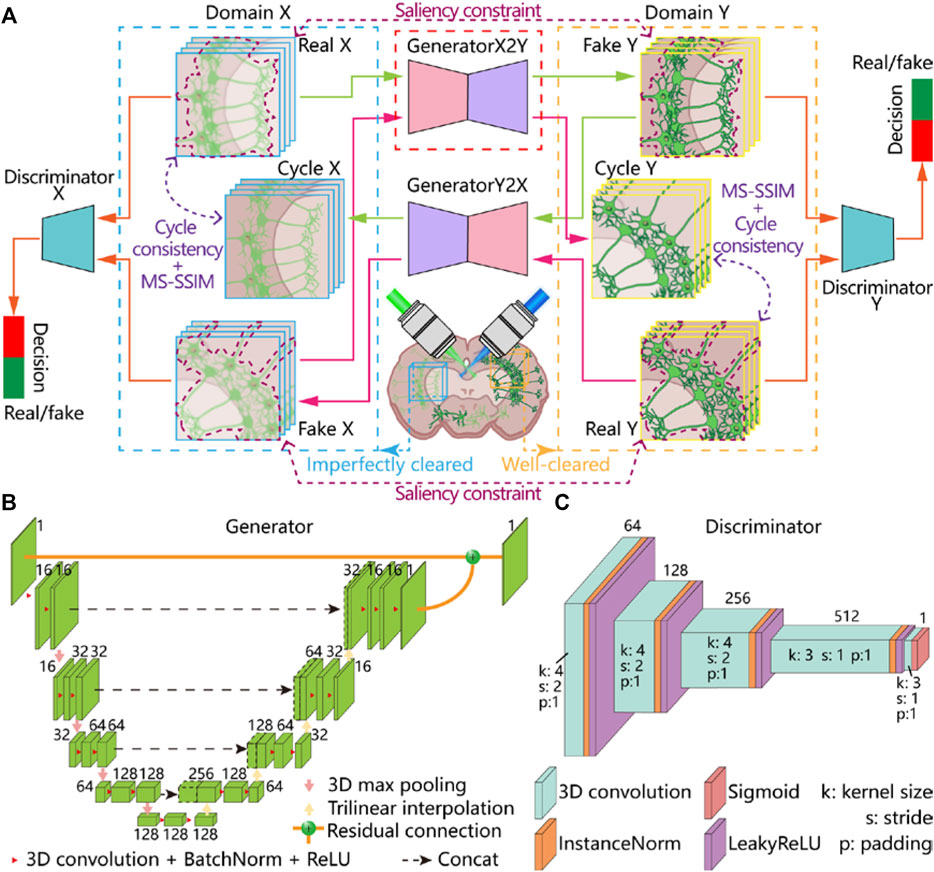
FIGURE 1. Framework of virtual optical clearing method and 3D-VoCycleGAN architecture. (A) The framework and workflow of our virtual optical clearing method. The 3D-VoCycleGAN consists of two generators and two discriminations (B) The network structure of generators. 3D ResUNet was used to build the two generators in our network (C) The network structure of discriminators. 3D PatchGAN was used to build the two discriminators in our network.
In the specific network training process, we defined the source domain and the target domain as domain X and domain Y, respectively. Taking the GPU memory requirements of network training into account, 200 groups of unpaired 3D image volumes with 256 × 256×16 pixel3 size were randomly cropped from the domain X and domain Y to generate the training datasets. In order to improve the training efficiency and avoid overfitting, image volumes with insufficient foreground were automatically discarded before training [33]. And these image volumes were normalized and then fed into the network for training. To ensure higher generalization capability of our network, during each training process, we performed data augmentation on the input image volumes by introducing a series of random changes, such as flipping, rotation, and so on. As the loss function iteratively minimized, the non-transparent 3D tissue image identified and learned the clearer structural features from the cleared 3D tissue image. After the deep learning network was well optimized, the original large LSFM image data with varying spatial transparency and contrast was sent to the network for implementing fast image prediction and image quality restoration.
3D-VoCycleGAN Architecture
In our 3D-VoCycleGAN, we built the two generators by using ResUNet, which has been proved to have great biological feature extraction capability [34]. The ResUNet used in our generators is a kind of encoder-decoder cascade structure, which is composed of four downsampling blocks and upsampling blocks (Figure 1B). In the encoder path, each downsampling block contained a max pooling and two convolution layers, each layer of which comprised 3 × 3×3 kernel followed by a batch-normalization layer and a ReLU activation function. And the encoder encoded the input image stack into multiple feature representations at different levels through max pooling. Then the decoder consisting of four upsampling blocks symmetrical to the encoder was used to decode data information back to the original dimension. Each upsampling block consisted of trilinear interpolation, skip connection, and convolution layers. The skip connection concatenated the high-level features and spatial information between encoder and decoder, thus retaining more details and capturing finer information. Finally, we established a residual connection between the input and the output of the decoder to avoid the gradient vanishing problem and improve the performance of the network [35].
For building the discriminators, we modified the five-layer conventional structure of PatchGAN [31] into a 3D form (Figure 1C). In the PatchGAN, conventional operation with a stride of 2 and padding of 1 was used in the first three conventional layers, each layer of which was followed by an instance normalization layer, and a LeakyReLU activation function. And the channel numbers were doubled as the image resolution was halved in the first three conventional each time. And the channel numbers of the five convolutional layers were 64, 128, 256, 512 and 1, respectively. Considering that the size of the input stack was 256 × 256×16, we set the kernel size of the last two convolution layers to 3 × 3×3, making the size of the output patch 32 × 32×2. Finally, the last convolutional layer reduced the channel numbers of the feature map to 1, and a sigmoid activation function was used to normalize the output value into [0, 1].
Our 3D-VoCycleGAN was implemented based on the Pytorch deep learning framework. The learning rate of the Adam optimizer was set to 0.0002 in the first 100 epochs and linearly decayed to 0 in the next 100 epochs. The batch size was set to 1. The overall training and prediction processes based on our method were implemented in a Dell 7,920 workstation equipped with RTX 3090 GPU (24 GB memory).
Loss Function
The deep learning model of 3D-VoCycleGAN contained two generators
where x denotes the blurred stack in domain X, y denotes the clear stack in domain Y.
The original cycle consistency loss calculated the L1 loss between the original image and reconstructed image. We incorporated a 3D multi-scale structural similarity index metric (MS-SSIM) to construct a detail preserving transformation [38]. The cycle consistency loss was defined as follows:
where
Saliency constraint has been proved to be effective for content preservation on 2D microscopic images [39]. And we added it to our 3D-VoCycleGAN for maintaining fine structures and information. By appropriately setting the threshold value, we could separate the foreground with detailed structure from the 3D samples. Therefore, the two generators focused on the essential structures of foreground at the early training stage and avoided appearance of artifacts in background with the aid of saliency constraint. The saliency constraint loss can be written as:
where
The total loss for generators could be expressed by:
where the parameters
Sample Preparation and 3D Image Data Acquisition
The sample used in this study contained mouse brain and mouse kidney tissues. For verifying the performance of our method on tissue slices, we prepared Thy1-GFP mouse brains and mouse kidney tissues, which were sectioned into 300-μm and 200-μm thick slices, respectively. The mouse kidney tissue slices were stained with DRAQ5 for labelling the cell nucleus before cleared by FOCM reagents. The FOCM reagents were prepared as 30% (wt/vol) urea (Vetec), 20% (wt/vol) D-sorbitol (Vetec), and 5% (wt/vol) glycerol dissolved in DMSO. When preparing the reagent, urea and D-sorbitol were dissolved in DMSO and stirred at room temperature overnight. After complete dissolution, glycerol was added and stirred further. The reagents should be stored at room temperature and shaken gently before using. Before imaging experiments, the well-stained mouse brain and kidney tissue slices were incubated in FOCM reagents for several minutes.
For verifying the performance of our method on deep tissues with millimeter-thickness, we prepared stereoscopic mouse brain and kidney tissue blocks labelled with Alexa Fluor 647 anti-mouse CD31 antibody (CD31-AF647, BioLegend) by caudal vein injection. The Alexa Fluor 647 anti-mouse CD31 antibody (20 mg) was then diluted in sterile saline (total volume of 150 ml). After the injection, mice were placed in a warm cage for 30 min prior to perfusion. Then mice were rapidly anesthetized with chloral hydrate [5%, wt/vol, 0.1 ml/10 g, intraperitoneal (i.p.)] and transcardially perfused with ice-cold 0.01 M phosphate buffered saline (PBS, Coolaber) and paraformaldehyde (PFA, 4% in PBS wt/vol, Saiguo Biotechnology Co., Ltd). Mouse brains and kidneys were collected and incubated in the same PFA solution at 4°C for 24–48 h for uniform fixation. After fixation, mouse brains and kidneys were washed in 0.01 M PBS at room temperature (20–25°C) for 6–12 h. The mouse brains and kidneys were clarified by the CUBIC-L/R+ protocol [xxx]. CUBIC-L [10 wt% of N-butyldiethanolamine (Vetec) and 10 wt% of Triton X-100 (Sigma) in water] and CUBIC-R+ [45 wt% of antipyrine (Vetec) and 30 wt% of nicotinamide (Vetec) in water, buffered with 0.5% (v/w) N-butyldiethanolamine (pH ∼ 10)] was prepared for tissue clearing. Mouse organs and tissues were incubated in CUBIC-L for 7 d at 37°C with gentle shaking followed by PBS washing at room temperature. After PBS clearing, the mouse brains and kidneys was incubated and stored in CUBIC-R+ at room temperature.
For generating 3D datasets and verifying the application of our method, we acquired the experimental data of mouse organs and tissues via a custom-built LSFM system. For exciting fluorescence signal of mouse tissues labeled with Thy1-GFP, DRAQ5, and CD31-AF647, two semiconductor lasers (OBIS 488LS/637LX nm, Coherent) were aligned and expanded by a pair of achromatic lenses with 30 and 250 mm focal length, respectively. Like the classical selective plane illumination microscopy, we used a cylindrical lens with 100 mm focal length and a low-NA objective (Olympus ×4/NA 0.1/WD 18.5 mm) with long working distance to generate a thin illumination sheet. And a mechanical slit (VA100 C/M, Thorlabs) was set to 1 mm for controlling the thickness of the illumination sheet. The fluorescence signal was collected by a tube lens (ITL200, Thorlabs), detection objective (Nikon ×4/NA 0.2/WD 20 mm), a multi-channel emission filter (#87-247, Edmund Optics) and a sCMOS camera (ORCA-Flash 4.0 V3, Hamamatsu). And the biological samples were loaded on a 3D motorized stage (KMT50SE/M-3D, Thorlabs) and performed scanned imaging. In this system, we used the external trigger mode with a synchronous signal to ensure high-frame image acquisition. During the LSFM imaging process, each frame was captured with a constant acquisition interval of 2 μm and total exposure time of 10 ms. The corresponding camera acquisition speed could be up to 100 fps. Due to the rapid imaging advantage, the image acquisition process of a whole mouse brain tissue slice could be finished in 4 min. All images were transformed and stored as 16-bit Multi-TIFF format for post-processing.
Results
Image Enhancement Performance of 3D-VoCycleGAN for Mouse Brain Slices
Due to spatial anisotropy and structural complexity of biological tissues, chemical tissue clearing still could not realize perfect tissue transparency and image contrast. As for a pre-cleared tissue, the clearing extent and spatial image degradation is random across the whole 3D volume. Here we first demonstrated our 3D-VoCycleGAN on Thy1-GFP mouse brain slices to digitally improve the optical clearing extent and image quality. Although the whole image showed the distribution of fluorescence signal in the brain slice, some details such as nerve fiber were still blurred as shown in Figure 2A. By using our 3D-VoCycleGAN, the image background was greatly suppressed. Besides, the blurred nerve fiber in the original image became more distinguishable after enhancement. Further, we cropped a region-of-interest (ROI) from the brain slice to compare the virtual optical clearing efficiency and image enhancing performance with other deconvolution methods. Here we performed sparse deconvolution [40], Richardson-Lucy deconvolution and 3D-VoCycleGAN on a 500 × 500×32 pixel3 image volume. According to the results in Figure 2B, three methods all realized image quality improvement to different extents. Then we plotted the profiles of two lines across the nerve fiber to quantitatively evaluate their differences of performance. Although Richardson-Lucy also enhanced the image resolution to some extent, the image background noise suppression capability was not as good as the other methods. Our 3D-VoCycleGAN and sparse deconvolution showed better image contrast and SBR improvements, which were both increased by above 40% (Figure 2C). It is worth noting that although sparse deconvolution showed very powerful image quality enhancing capability comparable to our 3D-VoCycleGAN, the processing time consumption for the image volume with same size is larger than our method (Figure 2D). It usually takes a considerable amount of time to finish the image processing by using Richardson-Lucy deconvolution. And sparse deconvolution could shorten the processing time with the aid of GPU acceleration. Nevertheless, due to GPU memory limitation, sparse deconvolution could not realize image processing of large 3D data in one time. Although sparse deconvolution could process the 3D image data volume by volume after splitting the large 3D image data into several image stacks, the final stitched 3D image will show uneven brightness and background since these sub-volumes exist sparsity differences. As for this image volume, the processing time consumption of 3D-VoCycleGAN, sparse deconvolution, and Richardson-Lucy deconvolution were 0.8, 48 and 45s, respectively. Thereinto, we performed 50 iterations of the Richardson-Lucy deconvolution by using the DeconvolutionLab2 plugin in ImageJ/Fiji. Then, with 3D-VoCycleGAN, image processing of the whole brain slice with 3,100 × 3,500×180 pixel3 volume could be finished in only 141s. Hence, our 3D-VoCycleGAN could realize great image quality enhancement with short time consumption, showing the great image processing efficiency in brain slice imaging.
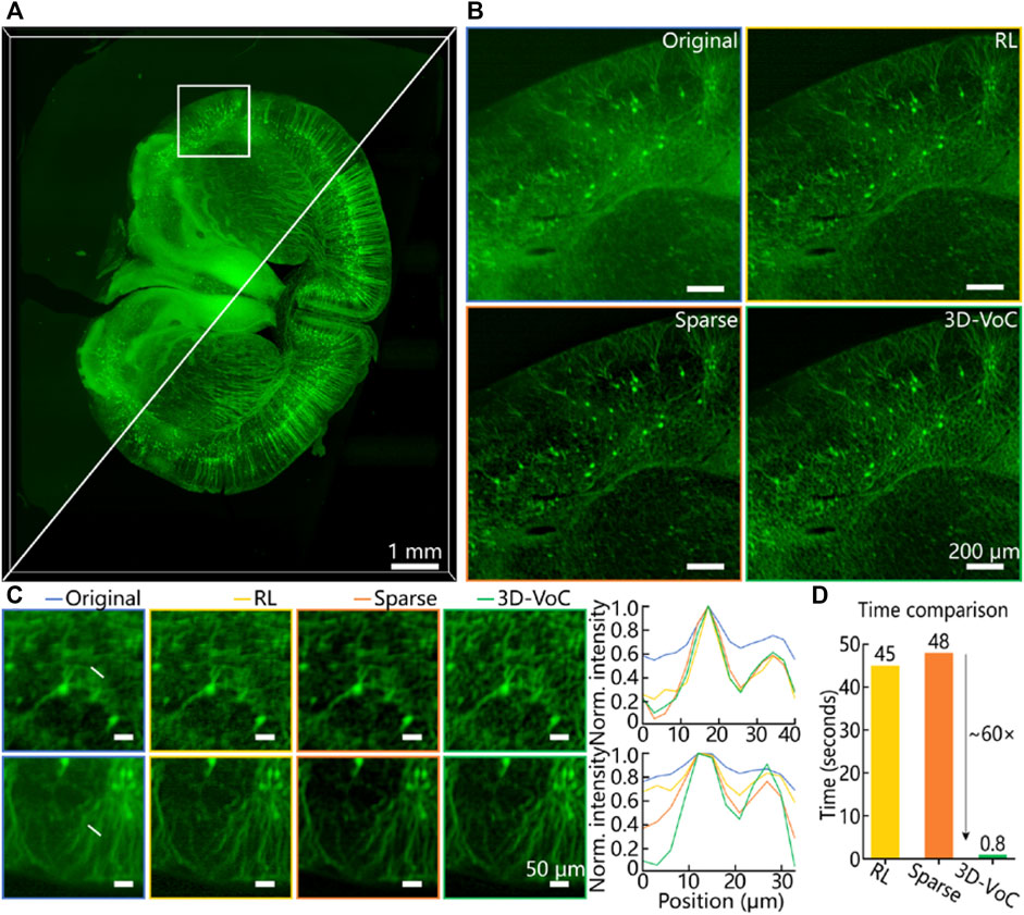
FIGURE 2. The image enhancement performance of 3D-VoCycleGAN. (A) The comparison results before and after using 3D-VoCyleGAN (B) The image quality enhancement results with Richardson-Lucy deconvolution, sparse deconvolution, and 3D-VoCycleGAN method. The size of cropped image volume was limited by the GPU memory requirements of Richardson-Lucy deconvolution and sparse deconvolution. (C) The quantitative evaluation of the image quality enhancement performance. The plotting curves of two line profiles showed the signal level and SBR of nerve fiber in the brain slice (D) The time consumption of different image processing methods for the image volume. RL: Richardson-Lucy deconvolution, Sparse: sparse deconvolution, 3D-VoC: 3D-VoCycleGAN.
Information Restoration of Images Deep Inside Kidney Tissue Slices
Tissue slice imaging with chemical optical clearing protocols are widely used in biological research. Although many chemical tissue clearing methods have promoted biological structure and function research, tissue scattering and refractive index mismatching between multiple media in the imaging system usually influence the image quality and microstructure analysis under the slice surface. Our 3D-VoCycleGAN could contribute to the information restoration of images deep inside tissue slices. As shown in Figure 3A, labelled cell nucleus of the mouse kidney tissue slice showed the distribution of glomeruli. However, the tissue transparency was not enough to distinguish the detailed nucleus or glomeruli. Especially, due to the uneven thickness and structural anisotropy in axial direction, the clearing reagents could not perfectly make the kidney tissue slice transparent. For example, although the kidney tissue slice could be optical cleared by the clearing reagents, the images deep inside the tissue slice were still blurred due to inevitable light scattering or attenuation. The fluorescence signal was nearly overwhelmed in the strong background signal except the area from the tissue surface to 115-μm depth (Figure 3B). By using our 3D-VoCycleGAN, the fluorescence signal in deep tissue could be quickly recovered. The axial images in Figures 3B,C showed the profile of glomeruli and tubules across about 150-μm depth, which improved the clearing depth of mouse kidney tissues by up to 30%. Besides, we could also compare the 2D images in different depths. When the imaging depth was 100 μm, the original image could show distinguished cell nucleus with faint noise. Our virtual optical clearing method could improve the image contrast with details maintained as shown in Figure 3D. When the imaging depth was 140 μm, the morphology of cell nucleus and glomeruli were severely blurred (Figure 3E). With 3D-VoCycleGAN, the final image quality was evidently improved, where some information of nucleus and glomeruli was recovered. Hence, to some extent, we could realize structural information restoration of imperfectly cleared tissue slices in deep depth by virtual optical clearing technique.
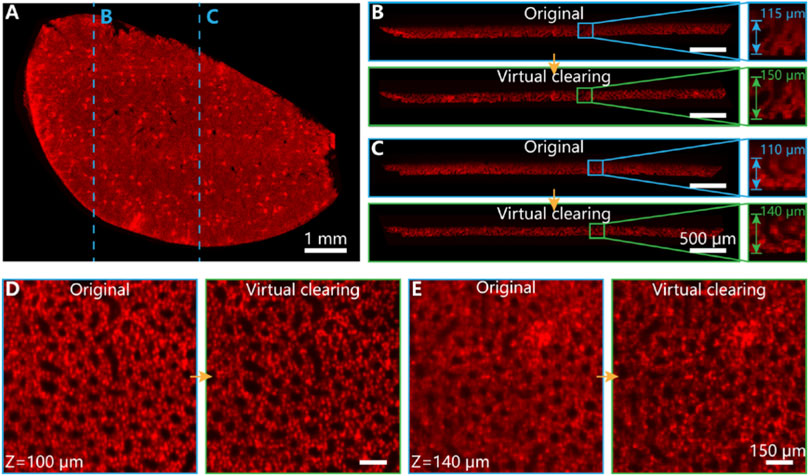
FIGURE 3. The image information restoration effect in a mouse kidney tissue slice. (A) Fluorescence image of a mouse kidney slice labelled with cell nucleus (B,C) The comparison of clearing extent between original and fluorescence image processed by 3D-VoCycleGAN. (D,E) The image improvements in different imaging depths. The image of z = 100 μm was given in (D) and image of z = 140 μm was given in (E).
Virtual Optical Clearing of Large-Scale 3D Tissues
Except for tissue slice imaging, high-throughput imaging for large-scale 3D tissues also plays an increasingly important part in biological research, especially in digital organ mapping and brain network reconstruction. Here we demonstrated the 3D image enhancement capability for stereoscopic mouse tissue with above 1 × 1 × 1 mm3 volume by using our virtual clearing method. To further depict the glomeruli distribution or morphology of kidney tissue, we imaged and reconstructed a mouse kidney tissue block with a custom-bulit LSFM system. As shown in Figure 4A, the original 3D image volume has evident space-variant opaqueness and structure blurring. In particular, the structural contours of glomeruli were gradually blurred as the axial depth increases, which was marked by the white arrow in Figure 4A. The connections between glomeruli and arteries were also very important for supporting some kidney functions. However, in the imperfectly cleared kidney tissue, a branch of the kidney artery was also overwhelmed in the background noise (yellow arrow in Figure 4A). By using our virtual optical clearing method, the glomeruli and artery branch were all evidently recovered and distinguished (Figure 4B). And the anisotropic tissue transparency was eliminated after virtual optical clearing. From the depth color-coded z-projections, we could see the whole image contrast and fluorescence signal intensity in various depths were enhanced (Figures 4C,D).
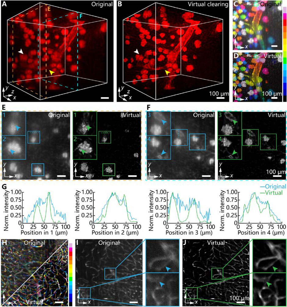
FIGURE 4. The virtual optical clearing effect for millimeter-thickness mouse tissues. (A) 3D fluorescence image of imperfectly cleared mouse kidney tissue. The two dashed boxes represents 2D sections from two imaging depths (B) 3D fluorescence image of virtually optically cleared mouse kidney tissue by using 3D-VoCycleGAN. The white and yellow arrows represents the glomerulus and artery branch, respectively. (C,D) The depth color-coded image of image volume in (A) and (B), respectively. (E) The comparison results between original image and virtually cleared image for shallow depth shown in (A). The magnifications of insets were ×2. (F) The comparison results between original image and virtually cleared image for deep depth shown in (A). The magnifications of insets were ×1.5. The blue and green arrows in (E) and (F) represented the structure details of glomeruli and artery branch, respectively. (G) The quantitative evaluation of tissue structural details. The plotting curves of four groups of line profiles represented the glomeruli and artery branch (H) The comparison results between original and virtually cleared mouse brain vessels by using depth color-coded z-projections. (I) The original 2D image showing blurred brain vessels (J) The 2D image corresponding to image (I) after virtual optical clearing. The blue and green arrows represented the brain vessel details. The magnifications of insets were ×3.
In order to quantify the virtual optical clearing effect, we selected two 2D images from two different z-depths. As shown in Figure 4E, the original 2D image had low image quality, including strong noise, blurring, and structure missing (two blue arrows). After virtual optical clearing, the details and contours of glomeruli were enhanced greatly, which might be meaningful to the morphological analysis of kidney microstructures. Although the original 2D image in Figure 4F had lower noise and blurring extent than the original image in Figure 4E because of shallow imaging depth, the vascular walls of two artery branches were still difficult to be distinguished directly (two green arrows). Our virtual optical clearing successfully recovered the details of two vascular walls. Further, we evaluated the fluorescence signal intensity and noise level in the two depths by plotting four lines. As shown in Figure 4G, images processed by our method had more distinguishable details about glomeruli and artery, especially the contour of glomeruli and vascular walls. Besides, our method improved the SBR of images by above 25%. Meanwhile, we tested our method on 3D images of brain vessels, which showed complex structures and dense distribution in the mouse brain. For deep brain tissue 3D imaging, tissue anisotropy and imperfect tissue clearing will introduce strong scattering and attenuation of fluorescence signal, resulting in vessel blurring and artifacts as shown in Figure 4H. According to the comparison results of depth color-coded z-projections, we could see the definition and sharpness of vessels were greatly improved in various depths by using our virtual optical clearing method. As shown in Figures 4I,J, the vessel artifacts were suppressed after virtual clearing. Similar to the results of kidney tissue, the original vessel contours existed severe blurring. Our virtual optical clearing method could effectively restore the information and improve the image quality, indicating its powerful image enhancement capability in 3D fluorescence imaging.
Discussion
High-throughput 3D fluorescence imaging and tissue clearing techniques are playing an increasingly important role in biological research. However, due to the tissue anisotropy and structural complexity, chemical tissue clearing techniques sometimes could not imperfectly clear the whole tissue, resulting in image quality degradation, such as image blurring, background noise, artifacts and so on. A series of methods including physical, chemical and digital ways have been proposed to improve the fluorescence image quality in recent years. Here, we presented an unsupervised deep learning-based image processing method, called 3D-VoCycleGAN to realize further virtual optical clearing of imperfectly cleared tissues. By making full use of the tissue anisotropy and space-variant clearing extent, we built a virtual optical clearing method to enhance the clearing effect of chemical tissue clearing techniques. In our virtual optical clearing, we established a CycleGAN architecture which consists of two pairs of 3D image generators and discriminators to realize the transformation and evaluation from low-quality LSFM images to high-quality LSFM images. Needless of accurate data pre-alignment between the source domain and target domain, our method need not accurate data pre-alignment between the source domain and target domain, which greatly improves the image processing efficiency. Compared with other image enhancement methods, our method showed more powerful image enhancement effect and faster processing speed. With the 3D-VoCycleGAN, we could restore more detailed mouse tissue structural information with high SBR and image contrast, such as distinguished nerve fibers, somas, glomeruli, and vessels.
Particularly, it is the first time that the CycleGAN deep learning model has been used for enhancing the clearing effect of chemical tissue clearing, and restoring the 3D blurred LSFM images. Furthermore, except for LSFM, our 3D-VoCycleGAN could also be used to process 3D images captured by other 3D fluorescence imaging systems such as confocal, two-photon microscopy and so on. From the aspect of deep learning network architecture, the 3D operations such as 3D max pooling and 3D convolution in our 3D-VoCycleGAN are not only limited to specific fluorescence imaging systems. From the aspect of dataset preparation, the sparse deconvolution method which we used to pre-process the 3D cleared tissue images was proposed to improve the image quality of structured illumination microscopy and proved to be available in various 3D fluorescence imaging systems such as confocal, two-photon, expansion microscopy and so on [40]. Hence, the whole image processing flow of our 3D-VoCycleGAN could be transferred to various 3D fluorescence imaging systems by using related datasets. In summary, our study promoted the combination and application of digital image processing, chemical tissue clearing and 3D fluorescence imaging techniques, showing the promising development of interdisciplinary technology in future high-throughput 3D biomedical imaging and biological research.
Data Availability Statement
The original contributions presented in the study are included in the article, further inquiries can be directed to the corresponding author.
Ethics Statement
All mouse experiments followed the guidelines for the Care and Use of Laboratory Animals of Zhejiang University approved by the Committee of Laboratory Animal Center of Zhejiang University.
Author Contributions
JC and ZD conceived the idea. KS supervised the project. JC and ZD performed the experiments and image processing. JC, ZD, and KS wrote the paper. All the authors contributed to the discussion on the results for this manuscript.
Funding
This work was supported in part by the Key R&D Program of Zhejiang Province (2021C03001), National Natural Science Foundation of China (61735016), CAMS Innovation Fund for Medical Sciences (2019-I2M-5-057), Fundamental Research Funds for the Central Universities, Alibaba Cloud.
Conflict of Interest
The authors declare that the research was conducted in the absence of any commercial or financial relationships that could be construed as a potential conflict of interest.
Publisher’s Note
All claims expressed in this article are solely those of the authors and do not necessarily represent those of their affiliated organizations, or those of the publisher, the editors and the reviewers. Any product that may be evaluated in this article, or claim that may be made by its manufacturer, is not guaranteed or endorsed by the publisher.
References
1. Wilson T, Sheppard C. Theory and Practice of Scanning Optical Microscopy. London: Academic Press (1984).
2. Feuchtinger A, Walch A, Dobosz M. Deep Tissue Imaging: A Review from a Preclinical Cancer Research Perspective. Histochem Cel Biol (2016) 146:781–806. doi:10.1007/s00418-016-1495-7
3. Ntziachristos V. Going Deeper Than Microscopy: The Optical Imaging Frontier in Biology. Nat Methods (2010) 7:603–14. doi:10.1038/nmeth.1483
4. Yu H, Rahim NAA. Imaging in Cellular and Tissue Engineering. 1st ed. Boca Raton: CRC Press (2013).
5. Yoon S, Kim M, Jang M, Choi Y, Choi W, Kang S, et al. Deep Optical Imaging within Complex Scattering media. Nat Rev Phys (2020) 2:141–58. doi:10.1038/s42254-019-0143-2
6. Helmchen F, Denk W. Deep Tissue Two-Photon Microscopy. Nat Methods (2005) 2:932–40. doi:10.1038/nmeth818
7. Li A, Gong H, Zhang B, Wang Q, Yan C, Wu J, et al. Micro-Optical Sectioning Tomography to Obtain a High-Resolution Atlas of the Mouse Brain. Science (2010) 330:1404–8. doi:10.1126/science.1191776
8. Dodt H-U, Leischner U, Schierloh A, Jährling N, Mauch CP, Deininger K, et al. Ultramicroscopy: Three-Dimensional Visualization of Neuronal Networks in the Whole Mouse Brain. Nat Methods (2007) 4:331–6. doi:10.1038/nmeth1036
9. Economo MN, Clack NG, Lavis LD, Gerfen CR, Svoboda K, Myers EW, et al. A Platform for Brain-wide Imaging and Reconstruction of Individual Neurons. eLife (2016) 5:e10566. doi:10.7554/eLife.10566
10. Wang H, Magnain C, Wang R, Dubb J, Varjabedian A, Tirrell LS, et al. as-PSOCT: Volumetric Microscopic Imaging of Human Brain Architecture and Connectivity. NeuroImage (2018) 165:56–68. doi:10.1016/j.neuroimage.2017.10.012
11. Stelzer EHK, Strobl F, Chang B-J, Preusser F, Preibisch S, McDole K, et al. Light Sheet Fluorescence Microscopy. Nat Rev Methods Primers (2021) 1:73. doi:10.1038/s43586-021-00069-4
12. Richardson DS, Guan W, Matsumoto K, Pan C, Chung K, Ertürk A, et al. Tissue Clearing. Nat Rev Methods Primers (2021) 1:84. doi:10.1038/s43586-021-00080-9
13. Brenna C, Simioni C, Varano G, Conti I, Costanzi E, Melloni M, et al. Optical Tissue Clearing Associated with 3D Imaging: Application in Preclinical and Clinical Studies. Histochem Cel Biol (2022) 157:497–511. doi:10.1007/s00418-022-02081-5
14. Yu T, Zhu J, Li D, Zhu D. Physical and Chemical Mechanisms of Tissue Optical Clearing. iScience (2021) 24:102178. doi:10.1016/j.isci.2021.102178
15. Matsumoto K, Mitani TT, Horiguchi SA, Kaneshiro J, Murakami TC, Mano T, et al. Advanced CUBIC Tissue Clearing for Whole-Organ Cell Profiling. Nat Protoc (2019) 14:3506–37. doi:10.1038/s41596-019-0240-9
16. Molbay M, Kolabas ZI, Todorov MI, Ohn T-L, Ertürk A. A Guidebook for DISCO Tissue Clearing. Mol Syst Biol (2021) 17:e9807. doi:10.15252/msb.20209807
17. Zhu X, Huang L, Zheng Y, Song Y, Xu Q, Wang J, et al. Ultrafast Optical Clearing Method for Three-Dimensional Imaging with Cellular Resolution. Proc Natl Acad Sci U.S.A (2019) 116:11480–9. doi:10.1073/pnas.1819583116
18. Cannell MB, McMorland A, Soeller C. Image Enhancement by Deconvolution. In: JB Pawley, editor. Handbook of Biological Confocal Microscopy. Boston, MA: Springer US (2006). p. 488–500. doi:10.1007/978-0-387-45524-2_25
19. Richardson WH. Bayesian-Based Iterative Method of Image Restoration*. J Opt Soc Am (1972) 62:55–9. doi:10.1364/josa.62.000055
20. Lucy LB. An Iterative Technique for the Rectification of Observed Distributions. Astronomical J (1974) 79:745. doi:10.1086/111605
21. Belthangady C, Royer LA. Applications, Promises, and Pitfalls of Deep Learning for Fluorescence Image Reconstruction. Nat Methods (2019) 16:1215–25. doi:10.1038/s41592-019-0458-z
22. Wang H, Rivenson Y, Jin Y, Wei Z, Gao R, Günaydın H, et al. Deep Learning Enables Cross-Modality Super-resolution in Fluorescence Microscopy. Nat Methods (2019) 16:103–10. doi:10.1038/s41592-018-0239-0
23. Zhang B, Zhu J, Si K, Gong W. Deep Learning Assisted Zonal Adaptive Aberration Correction. Front Phys (2021) 8. doi:10.3389/fphy.2020.621966
24. Schmidhuber J. Deep Learning in Neural Networks: An Overview. Neural Networks (2015) 61:85–117. doi:10.1016/j.neunet.2014.09.003
25. Jin KH, McCann MT, Froustey E, Unser M. Deep Convolutional Neural Network for Inverse Problems in Imaging. IEEE Trans Image Process (2017) 26:4509–22. doi:10.1109/tip.2017.2713099
26. Salim UT, Ali F, Dawwd SA, System D. U-net Convolutional Networks Performance Based on Software-Hardware Cooperation Parameters: A Review. Int J Comput Digital Syst (2021) 11. doi:10.12785/ijcds/110180
27. Karhunen J, Raiko T, Cho K. Unsupervised Deep Learning. In: E Bingham, S Kaski, J Laaksonen, and J Lampinen, editors. Advances in Independent Component Analysis and Learning Machines. Academic Press (2015). p. 125–42. doi:10.1016/b978-0-12-802806-3.00007-5
28. Li Z, Zhang T, Wan P, Zhang D. SEGAN: Structure-Enhanced Generative Adversarial Network for Compressed Sensing MRI Reconstruction. Proceedings of the AAAI Conference on Artificial Intelligence (2019) 33:1012–9. doi:10.1609/aaai.v33i01.33011012
29. Lv J, Wang C, Yang G. PIC-GAN: A Parallel Imaging Coupled Generative Adversarial Network for Accelerated Multi-Channel MRI Reconstruction. Diagnostics (2021) 11:61. doi:10.3390/diagnostics11010061
30. Quan TM, Nguyen-Duc T, Jeong W-K. Compressed Sensing MRI Reconstruction Using a Generative Adversarial Network with a Cyclic Loss. IEEE Trans Med Imaging (2018) 37:1488–97. doi:10.1109/tmi.2018.2820120
31. Zhu J-Y, Park T, Isola P, Efros AA. Unpaired Image-To-Image Translation Using Cycle-Consistent Adversarial Networks. In: IEEE International Conference on Computer Vision (ICCV); 22-29 October, 2017; Venice, Italy (2017). p. 2242–51. doi:10.1109/ICCV.2017.244
32. Li M, Huang H, Ma L, Liu W, Zhang T, Jiang Y. Unsupervised Image-To-Image Translation with Stacked Cycle-Consistent Adversarial Networks. In: Proceedings of the European conference on computer vision (ECCV); 8-14 September, 2018; Munich, Germany (2018). p. 184–99. doi:10.1007/978-3-030-01240-3_12
33. Chen J, Sasaki H, Lai H, Su Y, Liu J, Wu Y, et al. Three-dimensional Residual Channel Attention Networks Denoise and Sharpen Fluorescence Microscopy Image Volumes. Nat Methods (2021) 18:678–87. doi:10.1038/s41592-021-01155-x
34. Weigert M, Schmidt U, Boothe T, Müller A, Dibrov A, Jain A, et al. Content-aware Image Restoration: Pushing the Limits of Fluorescence Microscopy. Nat Methods (2018) 15:1090–7. doi:10.1038/s41592-018-0216-7
35. He K, Zhang X, Ren S, Sun J. Deep Residual Learning for Image Recognition. In: Proceedings of the IEEE conference on computer vision and pattern recognition; 27-30 June 2016; Las Vegas, NV, USA (2016). p. 770–8. doi:10.1109/cvpr.2016.90
36. Goodfellow I, Pouget-Abadie J, Mirza M, Xu B, Warde-Farley D, Ozair S, et al. Generative Adversarial Nets. Adv Neural Inf Process Syst (2014) 2:2672–80. doi:10.5555/2969033.2969125
37. Mao X, Li Q, Xie H, Lau RY, Wang Z, Paul Smolley S. Least Squares Generative Adversarial Networks. In: Proceedings of the IEEE international conference on computer vision; 22-29 October, 2017; Venice, Italy (2017). 2794–802. doi:10.1109/iccv.2017.304
38. Wang Z, Simoncelli EP, Bovik AC. Multiscale Structural Similarity for Image Quality Assessment. In: The Thrity-Seventh Asilomar Conference on Signals, Systems & Computers; November 09-12, 2003; Pacific Grove,CA (2003). p. 1398–402. doi:10.1109/ACSSC.2003.1292216
39. Li X, Zhang G, Qiao H, Bao F, Deng Y, Wu J, et al. Unsupervised Content-Preserving Transformation for Optical Microscopy. Light Sci Appl (2021) 10:44. doi:10.1038/s41377-021-00484-y
Keywords: optical clearing, deep learning, deep tissue imaging, light-sheet, image processing
Citation: Chen J, Du Z and Si K (2022) Three-Dimensional Virtual Optical Clearing With Cycle-Consistent Generative Adversarial Network. Front. Phys. 10:965095. doi: 10.3389/fphy.2022.965095
Received: 09 June 2022; Accepted: 22 June 2022;
Published: 19 July 2022.
Edited by:
Liwei Liu, Shenzhen University, ChinaReviewed by:
Ming Lei, Xi’an Jiaotong University, ChinaSihua Yang, South China Normal University, China
Copyright © 2022 Chen, Du and Si. This is an open-access article distributed under the terms of the Creative Commons Attribution License (CC BY). The use, distribution or reproduction in other forums is permitted, provided the original author(s) and the copyright owner(s) are credited and that the original publication in this journal is cited, in accordance with accepted academic practice. No use, distribution or reproduction is permitted which does not comply with these terms.
*Correspondence: Ke Si, kesi@zju.edu.cn
†These authors have contributed equally to this work