The modified finite element method for heat and mass transfer of unsteady reacting flow with mixed convection

This study reveals the extension of a mathematical model of heat and mass transfer of fluid flow over a sheet by incorporating the effect of non-linear mixed convection. The governing equations of flow phenomena are expressed as partial differential equations (PDEs). Similarity transformations are employed to get a dimensionless set of boundary value problems. Most of the existing relevant literature employed some solver to solve a set of differential equations, but this study implements the finite element method to tackle the boundary value problems. The employed finite element method is based on the Galerkin approach. For verifications of the obtained results, a set of linear and non-linear boundary value problems is also solved with Matlab solver $bvp4c$. The results are displayed in graphs by varying Grashof number, modified (solutal) Grashof number, non-linear convection parameters in heat and mass transfer, radiation parameter, Prandtl number, Schmidt number, and reaction rate parameter. Also, numerical values for the friction at the wall and local Nusselt and Sherwood numbers are given in tables. The problem in PDEs form is also solved with software that implements the finite element method to solve problems. The simulations are also provided, which is the outcome of the software. It is shown that the velocity profile escalates by growing values of thermal and solutal Grashof numbers. Problem-solving techniques from this study may be used in future research to address other unsolved heat transfer fluid physics issues.

Introduction

Mathematical modeling of physical processes is substantial in engineering because these are constructed to express the physical situation to its equivalent mathematical form. Fluid mechanics is the field that utilizes mathematical modeling to convert a physical problem to its corresponding mathematical expression. Additionally, it provides solutions to the models and the quantitative description for which the model was constructed. These solutions explained the behavior of different quantities when variable parameters were used in the equation. The fluid’s velocity, pressure, temperature, and concentration could be the quantities in fluid dynamics.

Today, the study of Newtonian fluid’s fluid flow and energy transfer has gravitated several mathematical researchers. The fluid that obeys Newton’s viscosity law is termed Newtonian fluid. This area of research in fluid mechanics has extensive applications in hot rolling, wire drawing, the boundary layer, liquid film, paper production, and polymeric industries. Hayat et al. [1] studied the unsteady MHD flow over an exponentially stretching surface. The boundary layer equations for this phenomenon have been reduced into ordinary differential equations using suitable transformations. Series solutions for velocity and temperature have been obtained and analyzed with respect to contained parameters. Mukhopadhyay [2] studied the MHD boundary layer flow under the heat transfer of viscous fluid over an exponentially stretching sheet. Bhattacharyya et al. [3] discussed the problem of heat transfer in stagnation point flow over an exponentially shrinking sheet. The numerical investigation of time-dependent flow with the characteristic of heat transfer under the effects of the magnetic field, internal heat generation, or absorption has been carried out by Elbashbeshy et al. [4].

One of the attractive fields in fluid mechanics is studying forced situations, and free convection coincides, called mixed convection. Mixed convection occurs when free convection is significant under forced flow or forced convection under buoyancy forces. Mixed convection has applications in engineering fields such as heat exchangers, solar collectors, contaminant particle deposition, electronic equipment transport processes, and atmospheric boundary layer flows. Bhattacharyya et al. [5] studied the mixed convective boundary layer flow having slip effects over a flat plate. For numerical solutions of the obtained non-linear equations, Galerkin weighted residual method was employed. Shehzad et al. [17] investigated three-dimensional mixed convective flows of an Oldroyd-B fluid over the bidirectional stretching surface under the effects of radiations using the Rosseland approximation. Mukhopadhyay et al. [6] explored the incompressible, laminar, viscous, axisymmetric boundary layer flow towards a stretching cylinder. Hayat et al. [7] studied the constant three-dimensional flow of viscoelastic fluid over an exponentially stretched surface under convective boundary conditions and heat radiation. An analytical method, namely homotopy analysis, has been employed by Rashidi et al. [8] to explore micropolar fluid’s mixed convective boundary layer flow over a heated shrinking surface.

Models in fluid mechanics were formulated with or without heat and mass transfer. Few models have converted partial differential equations into ordinary differential equations utilizing equivalent similarity transformation. This conversion involved those fluids which have a similar flow. Modeling in fluid mechanics was constructed using Navier Stock equations based on Newton’s second law of motion. The study of small fluid elements, control volume, and 3D force can be done using the Navier stock equation. The mathematical form of Newton’s second law of motion revealed the cluster of forces acting on control volume.

Navier stokes equation consists of the sum of all forces acting on a flow and the product of mass and acceleration. These forces are gravitational, differential pressure, and force due to viscosity. These can be considered small fluid elements. Applying the chain rule to acceleration helps generate the convective components of acceleration [9–12]. Have studied the energy and mass transfer in mixed convection and elaborated the parameters (velocity, temperature, and concentration profile) using a chemical reaction.

Applications of fluid flow convection include chemical, food, fire control, petroleum reservoirs, and extraction of metals from their ores. In [13–15], Kh. Abdul Maleque worked on Arrhenius activation energy by considering binary chemical reactions with exothermic/endothermic properties. Natural convection was converted into an ordinary differential equation using the similarity technique. However, he introduced some non-dimensional variables and achieved similarity by assumption. In [16], the author used Oldroyd-B fluid to investigate three-dimensional mixed convected flow in the presence of thermal rays. Analytical issues were solved using the homotopy analysis method.

Unsteady nanofluid flow over the wedge under the effects of non-linear mixed convection has been studied in [17] using Matlab solver bvp4c. The Buongiorno model com-prises the effects of Brownian diffusion and thermophoresis. It was concluded that the impact of the non-linear convection parameter for temperature was more than that of concentration. An inclined MHD flow of a Micropolar fluid has been studied in [18] using the effects of the porous medium, transportation of heat and mass, and thermal radiations. The results reveal that the micropolar fluid flow depended on the mentioned effects. An analytical study for heat transfer of MHD flow over a stretching sheet has been given [19]. Two types of temperature conditions have been discussed. One was prescribed surface temperature, and another was named wall heat flux.

The exact solution for the non-linear ordinary differential equation obtained by employing similarity transformations on the momentum boundary layer equation was found. Other than numerical and analytical approximate solutions, exact solutions for some flow problems have been found in the literature. In [20], an exact and analytical approximate solution of Axisymmetric flow over a radially stretching sheet using the effects of heat transfer has been found. The sheet was porous, and the flow was generated due to the stretchiness of the sheet. The incomplete Gamma function found the exact solutions of the system of equations obtained by employing similarity transformations on the governing equations of the flow problem. Some flow problems have dual solutions. Among them, dual solutions for an equation for mixed convection in a porous medium have been considered [21]. The lower branch of the solution was terminated with a specified parameter value, and it also had essential singularity. Both solutions were shown to be bifurcated from the single solution. It was also shown that the upper branch of solutions was stable while the lower branch of solutions was unstable. An asymptotic solution was obtained in [22] for the natural convection of a nanofluid in a porous enclosure under a magnetic field and internal heating. This phenomenon has been applied in a plethora of bioengineering and industrial applications. This type of case was more physically realistic. Effects of some parameters in a transformed set of ordinary differential equations on fluid flow and heat transfer were graphically presented. For certain ranges of parameters, dual solutions of the system of ordinary differential equations were found.

The study of heat and mass transfer for the flow of three-dimensional Oldroyd-B fluid under the influence of Soret and Dufour over a bidirectional stretching sheet has been given in [23]. The Runge–Kutta-Fehlberg scheme has been employed to solve the differential equations. The results revealed that rising Deborah number values positively impact the temperature rate. The study of Maxwell liquid over a stretching sheet under the effects of magnetic dipole and thermophoretic particle has been provided in [24]. Later, suitable transformations have been employed to transform the dimensional partial differential equations into dimensionless ordinary differential equations. This shooting technique is based on Runge-Kutta Fehlberg 45 approach for solving the ordinary differential equation. It was concluded that the velocity gradient deteriorated by the increasing ferromagnetic interaction parameter. The Koo and Kleinstreuer-Li (KKL) nanofluid model has been studied in [25]. The mathematical model of ferromagnetic nanofluid flow was established under the effect of the chemical reaction and porous medium. The shooting method was adopted to solve dimensionless ordinary differential equations. The results revealed that velocity gradient decayed by rising values of ferromagnetic interaction parameter.

The domains of engineering, manufacturing, and biomedicine are just some of the many applications that make extensive use of hybrid nanofluids. For these applications [26], addressed the non-Fourier heat flux model for the flow of AA7072/AA7075/water-based hybrid nanofluids over curved stretching sheets. More work on fluid flow in the form of PDEs can be seen in [27–29].

Due to FEM’s great precision, it is a necessary numerical method for solving the non-linear system of ordinary differential equations (ODEs) that depicts heat transport from a thin liquid film accompanied by thermal radiations and a magnetic field. Here, the heat and mass transportation model of chemically reactive fluid flow over the sheet is extended by considering a non-linear mixed convection effect. The model is further reduced to ordinary differential equations with boundary conditions. Various solution methodologies exist for these kinds of linear and non-linear differential equations. But the current approach uses the modified finite element method to study the effect of parameters on velocity, temperature, and concentration profiles. The obtained equations are also tackled with Matlab solver bvp4c. This Matlab solver provides high-order accurate solutions for boundary values problems. Since the Matlab solver must use only first-order differential equations, all the second-order equations are reduced into a set of first-order equations. The main advantage of using a solver is to handle boundary value problems. The Galerkin-based approach modified finite element method is employed using first-degree polynomial interpolation. Rather than strong formulations, weak formulations are considered. Afterward, a matrix-vector equation is obtained containing the stiffness matrix. The stiffness matrix contains matrices obtained by finding integrals of some expressions. For getting quick results, a numerical integration approach is considered. This numerical approach is based on Gauss quadrature that uses points obtained from Legendre’s third-degree polynomial. For non-linear terms, an iterative procedure is adopted that stops when stopping criteria are met. So, in this manner, the system of a linear and non-linear set of boundary value problems is solved by employing the modified finite element method and Matlab solver bvp4c.

Problem formulation

Consider unsteady, incompressible, laminar, unsteady and Newtonian flow over a stretching sheet. Let the sheet be stretched with velocity $u_0$. Let $x$-axis be kept along the plate, whereas $y$-axis be placed perpendicular to $x$-axis. The stretchiness of the sheet generates the flow. Consider the non-linear mixed convection flow, and under the assumption of boundary layer theory that considers Reynolds number to fall in some particular range, the governing equations of the flow can be expressed as:

$\frac{\partial v}{\partial y}=0\left(\mathrm{Continuity}\mathrm{equation}\mathrm{for}\mathrm{this}\mathrm{case}\right)(1)$

$\frac{\partial u}{\partial t}+v\frac{\partial u}{\partial y}=\nu \frac{{\partial }^{2}u}{\partial y^2}+g\left(\begin{array}{c}{\mathrm{\Lambda }}_1\left(T-T_{\infty }\right)\\ +{\mathrm{\Lambda }}_2{\left(T-T_{\infty }\right)}^2\end{array}\right)+g\left(\begin{array}{c}{\mathrm{\Lambda }}_3\left(C-C_{\infty }\right)\\ +{\mathrm{\Lambda }}_4{\left(C-C_{\infty }\right)}^2\end{array}\right)\left(x-\mathrm{Momentum}\mathrm{equation}\right)(2)$

$\frac{\partial T}{\partial t}+v\frac{\partial T}{\partial y}=\alpha \frac{{\partial }^{2}T}{\partial y^2}-\frac{\mathit{1}}{e{c}_p}\frac{\partial q_r}{\partial y}\left(\mathrm{E}\mathrm{n}\mathrm{e}\mathrm{r}\mathrm{g}\mathrm{y}\mathrm{e}\mathrm{q}\mathrm{u}\mathrm{a}\mathrm{t}\mathrm{i}\mathrm{o}\mathrm{n}\right)(3)$

$\frac{\partial C}{\partial t}+v\frac{\partial C}{\partial y}=D\frac{{\partial }^{2}C}{\partial y^2}-k_1\left(C-C_{\infty }\right)\left(\mathrm{C}\mathrm{o}\mathrm{n}\mathrm{c}\mathrm{e}\mathrm{n}\mathrm{t}\mathrm{r}\mathrm{a}\mathrm{t}\mathrm{i}\mathrm{o}\mathrm{n}\mathrm{e}\mathrm{q}\mathrm{u}\mathrm{a}\mathrm{t}\mathrm{i}\mathrm{o}\mathrm{n}\right)(4)$

In Eqs 1–4, the effects of thermal radiations and chemical reactions are also considered where it is assumed that all derivatives with respect to $x$ are ignored [14]. The geometry of the problem is shown in Figure 1. Figure 1 shows three boundary layers, the flow direction and temperature and concentration at the wall and free stream.

FIGURE 1

FIGURE 1. Geometry of the problem with streamwise and cross-streamwise coordinates.

Eqs 1–4 are considered subject to the boundary conditions

$\begin{array}{c}u\left(t,y\right)=U_0,v=v_w\left(t\right),T=T_w,C=C_{w}wheny=0,t>0\\ u\left(t,y\right)\to 0,T\to T_{\infty },C\to C_{\infty }wheny\to \infty t>0\end{array}\}(5)$

In Eqs 1–4, $u\&v$ represent the horizontal and vertical velocity of the flow, respectively, $T$ represents the temperature of the fluid, $C$ denotes concentration, $T_w\&C_w$ are respectively temperatures and concentration at the sheet, $T_{\infty }\&C_{\infty }$ are respectively temperature of the fluid and concentration at the free stream, $\nu$ denotes kinematic viscosity, $g$ be the gravity, ${\Lambda }_1\&{\Lambda }_2$ denote linear and non-linear thermal expansion coefficients, ${\Lambda }_3\&{\Lambda }_4$ denote linear and non-linear solutal expansion coefficients, $q_r$ be the radiative flux, $\alpha$ be the thermal diffusivity, $\rho$ be the density, $c_p$ is the specific heat capacity, $D$ is the thermal diffusivity and $k_1$ is the reaction rate. Let the linearized Rosseland [30] radiative flux $q_r$ is expressed as:

$q_r=-\frac{16{\sigma }^{\ast }{T}_{\infty }^3}{3k^{\ast }}\frac{\partial T}{\partial y}$

where ${\sigma }^{\ast }$ is Stefan Boltzmann constant and $k^{*}$ is mean absorption coefficient.The following transformations are considered [14]:

$\eta =\frac{y}{\delta \left(t\right)},u=U_{0}f\left(\eta \right),\theta =\frac{T-T_{\infty }}{T_w-T_{\infty }},\varphi =\frac{C-C_{\infty }}{C_w-C_{\infty }}(6)$

It is given in [14] that the solution of Eq. 1 can be expressed as:

$v=\frac{v_0\nu }{\delta \left(t\right)}(7)$

where $v_0=-\frac{v_w\delta }{\nu }$ is dimensionless suction/injection velocity of the plate.

Substituting transformations Eq. 6 into Eqs 2–5 yields

$f^{″}+\left(\frac{\eta \delta {\delta }^{\prime }}{\nu }+v_0\right)f^{\prime }+Gr\left(\theta +{\beta }_1{\theta }^2\right)+Gm\left(\varphi +{\beta }_1{\varphi }^2\right)=0(8)$

$\frac{1}{P_r}\left(1+\frac{4}{3}{R}_d\right){\theta }^{″}+{\theta }^{\prime }\left(\eta \frac{\delta {\delta }^{\prime }}{\nu }+v_0\right)=0(9)$

$\frac{1}{S_c}{\varphi }^{″}+{\varphi }^{\prime }\left(\eta \frac{\delta {\delta }^{\prime }}{\nu }+v_0\right)-\gamma \varphi =0(10)$

Subject to the boundary conditions

$\begin{array}{c}f\left(\eta \right)=\mathit{1},\theta \left(\eta \right)=\mathit{1},\varphi \left(\eta \right)=1when\eta =\mathit{0}\\ f\left(\eta \right)\to 0,\theta \left(\eta \right)\to 0,\varphi \left(\eta \right)\to 0when\eta \to \infty \end{array}\}(11)$

where $Gr=\frac{g{\Lambda }_1\left(T_w-T_{\infty }\right){\delta }^2}{\nu U_0},Gm=\frac{g{\Lambda }_3\left(C_w-C_{\infty }\right){\delta }^2}{\nu U_0},{\beta }_1=\frac{{\Lambda }_2}{{\Lambda }_1}\left(T_w-T_{\infty }\right),{\beta }_2=\frac{{\Lambda }_4}{{\Lambda }_3}\left(C_w-C_{\infty }\right),P_r=\frac{\nu }{\gamma },R_d=\frac{4{\sigma }^{*}{T}_{\infty }^3}{k{k}^{*}},\gamma =\frac{k_1{\delta }^2}{\nu },S_C=\frac{\nu }{D}$

Denotes the Grashof number, the modified (solutal) Grashof number, non-linear thermal convection variable, Prandtl number, radiation parameter, non-dimensional reaction rate, and Schmidt number, respectively. In $R_d$ denotes the thermal conductivity. Since Eqs 8–10 contains the term $\frac{\delta {\delta }^{\prime }}{\nu }$ which will be treated as constant [14] for the requirement of the similarity conditions. Therefore,

$\frac{\delta {\delta }^{\prime }}{\nu }=A(12)$

So, Re-write Eqs 8–10 as

$f^{″}+\left(\eta A+v_0\right)f^{\prime }+Gr\left(\theta +{\beta }_1{\theta }^2\right)+Gm\left(\varphi +{\beta }_1{\varphi }^2\right)=0(13)$

$\frac{1}{P_r}\left(1+\frac{4}{3}{R}_d\right){\theta }^{″}+{\theta }^{\prime }\left(\eta A+v_0\right)=0(14)$

$\frac{1}{S_c}{\varphi }^{″}+{\varphi }^{\prime }\left(\eta A+v_0\right)-\gamma \varphi =0(15)$

Under the same boundary conditions as those specified in Eq. 11. The coefficient of skin friction, the local Nusselt number, and the local Sherwood number are defined as follows: $C_f=\frac{\tau }{{2\rho \mathrm{U}}_{\circ }^2}$ where $\tau =-\mu {\left(\frac{\partial u}{\partial y}\right)}_{y=0}=-\frac{\mu U_0}{\delta }{f}^{\prime }\left(\eta \right)$$N_u=\frac{q_w\delta }{k\left(T_w-T_{\infty }\right)}$ and $S_h=\frac{M_w\delta }{D\left(C_w-C_{\infty }\right)}$ where $q_w=-\left(k+\frac{16{\sigma }^{*}{T}_{\infty }^3}{3k^{*}}\right){\left(\frac{\partial T}{\partial y}\right)}_{y=0}=-\left(k+\frac{16{\sigma }^{*}{T}_{\infty }^3}{3k^{*}}\right)\frac{\left(T_w-T_{\infty }\right)}{{\delta }_t}{\theta }^{\prime }\left(0\right)$ and $M_w=-D{\left(\frac{\partial C}{\partial y}\right)}_{y=0}=-\frac{\left(C_w-C\right)}{{\delta }_t}{\varphi }^{\prime }\left(0\right)$Thus

$\frac{1}{2}{R}_e{C}_f=-f^{\prime }\left(0\right)(16)$

$N_u=-\left(1+\frac{4}{3}{R}_d\right){\theta }^{\prime }\left(0\right)(17)$

$S_h=-{\varphi }^{\prime }\left(0\right)(18)$

where $R_e=\frac{U_0\delta }{\nu }$ denotes the Reynolds numbers.

Finite element method

The dimensionless system of boundary value problems (13)-(15) using boundary condition (11) are solved by the numerical technique finite element method. Solving problems using this whole method domain that is infinitely long is considered the finite domain. Let it be divided into an equal subdomain called the element. Let $h$ be the length of each element, and every element is constructed on two nodes at its left and right endpoint. Let the solution be approximated by the interpolation of linear polynomials of the forms

$f=a_0+a_1\eta ,\theta =b_0+b_1{\eta }_1,\varphi =c_0+c_1\eta (19)$

Where $a_0,a_1,b_0,b_1,c_0\&c_1$are unknowns which will be determined by considering the values of $f,\theta \&\varphi$ at two nodes of $ith$element, the values of the unknown in Eq. 19 can be found and so solving approximation for $f,\theta \&\varphi$ can be obtained as:

$\begin{array}{c}f={\psi }_1\left(\eta \right)f_i+{\psi }_2\left(\eta \right)f_{i+1}\\ \theta ={\psi }_1\left(\eta \right){\theta }_i+{\psi }_2\left(\eta \right){\theta }_{i+1}\\ \varphi ={\psi }_1\left(\eta \right){\varphi }_i+{\psi }_2\left(\eta \right){\varphi }_{i+1}\end{array}\}(20)$

where

${\psi }_1\left(\eta \right)=\frac{{\eta }_{i+1}-\eta }{{\eta }_{i+1}-{\eta }_i},{\psi }_2\left(\eta \right)=\frac{\eta -{\eta }_i}{{\eta }_{i+1}-{\eta }_i}\mathrm{for}{\eta }_i\le \eta \le {\eta }_{i+1}(21)$

where ${\psi }_1\left(\eta \right)$ and ${\psi }_2\left(\eta \right)$ are called shape functions, and $f,\theta \&\varphi$ are called trail functions.

Using the Galerkin finite element method, weighted residuals of Eqs 13–15 are constructed as

$\underset{0}{\overset{{\eta }_{\infty }}{{\displaystyle \int }}}\psi \left(\frac{d^{2}f}{d{\eta }^2}+\left(A\eta +v_0\right)\frac{df}{d\eta }+G_{{\gamma }_L}\theta +{\beta }_1{G}_{{\gamma }_L}\theta \overline{\theta }+G_{{\gamma }_C}\varphi +{\beta }_2{G}_{{\gamma }_C}\varphi \overline{\varphi }\right)d\eta =0(22)$

$\underset{0}{\overset{{\eta }_{\infty }}{{\displaystyle \int }}}\psi \left(\frac{1}{P_r}\left(1+\frac{4}{3}{R}_d\right)\frac{d^2\theta }{d{\eta }^2}+\frac{d\theta }{d\eta }\left(\eta A+v_0\right)\right)d\eta =0(23)$

$\underset{0}{\overset{{\eta }_{\infty }}{{\displaystyle \int }}}\psi \left(\frac{1}{S_c}\frac{d^2\varphi }{d{\eta }^2}+\frac{d\varphi }{d\eta }\left(\eta A+v_0\right)-\gamma \varphi \right)d\eta =0(24)$

The trial function in Eqs 22–24 will be considered by using Eq. 20, and the test function is the vector of the form $\psi ={\left[{\psi }_1\left(\eta \right),{\psi }_2\left(\eta \right)\right]}^t$. Eqs 22–24 are strong formulations. For getting weak formulations, integration by parts will be carried out. Therefore, weal formulations can be expressed as:

$\underset{0}{\overset{{\eta }_{\infty }}{{\displaystyle \int }}}-\frac{d\psi }{d\eta }\frac{df}{d\eta }+\psi \left\{\begin{array}{c}\left(A\eta +v_{\circ }\right)\frac{df}{d\eta }+G_{{\gamma }_L}\theta +{\beta }_1{G}_{{\gamma }_L}\theta \overline{\theta }\\ +G_{{\gamma }_C}\varphi +{\beta }_2{G}_{{\gamma }_C}\varphi \overline{\varphi }\end{array}\right\}d\eta ={\left(\psi \frac{df}{d\eta }\right)}_0^{{\eta }_{\infty }}(25)$

$\underset{0}{\overset{{\eta }_{\infty }}{{\displaystyle \int }}}-\frac{1}{P_r}\left(1+\frac{4}{3}{R}_d\right)\frac{d\psi }{d\eta }\frac{d\theta }{d\eta }+\psi \left\{\frac{d\theta }{d\eta }\left(\eta A+v_{\circ }\right)\right\}d\eta ={\left(\psi \frac{d\theta }{d\eta }\right)}_0^{{\eta }_{\infty }}\frac{1}{P_r}\left(1+\frac{4}{3}{R}_d\right)(26)$

$\underset{0}{\overset{{\eta }_{\infty }}{{\displaystyle \int }}}-\frac{1}{S_c}\frac{d\psi }{d\eta }\frac{d\varphi }{d\eta }+\psi \left\{\frac{d\varphi }{d\eta }\left(\eta A+v_{\circ }\right)-\gamma \varphi \right\}d\eta ={\left(\psi \frac{d\varphi }{d\eta }\right)}_0^{{\eta }_{\infty }}\frac{1}{S_C}(27)$

The weak formulations Eqs 25–27 are constructed on the whole domain. For their construction on a single element $″i″$ the following equations can be constructed.

$\underset{{\eta }_i}{\overset{{\eta }_{i+1}}{{\displaystyle \int }}}-\frac{d\psi }{d\eta }\frac{df}{d\eta }+\psi \left\{\begin{array}{c}\left(A\eta +v_0\right)\frac{df}{d\eta }+G_{{\gamma }_L}\theta +\\ {\beta }_1{G}_{{\gamma }_L}\theta \overline{\theta }+G_{{\gamma }_C}\varphi +{\beta }_2{G}_{{\gamma }_C}\varphi \overline{\varphi }\end{array}\right\}d\eta ={\left(\psi \frac{df}{d\eta }\right)}_{{\eta }_i}^{{\eta }_{i+1}}(28)$

$\underset{{\eta }_i}{\overset{{\eta }_{i+1}}{{\displaystyle \int }}}-\frac{1}{P_r}\left(1+\frac{4}{3}{R}_d\right)\frac{d\psi }{d\eta }\frac{d\theta }{d\eta }+\psi \left\{\frac{d\theta }{d\eta }\left(\eta A+v_0\right)\right\}d\eta ={\left(\psi \frac{d\theta }{d\eta }\right)}_{{\eta }_i}^{{\eta }_{i+1}}\frac{1}{P_r}\left(1+\frac{4}{3}{R}_d\right)(29)$

$\underset{{\eta }_i}{\overset{{\eta }_{i+1}}{{\displaystyle \int }}}-\frac{1}{S_c}\frac{d\psi }{d\eta }\frac{d\varphi }{d\eta }+\psi \left\{\frac{d\varphi }{d\eta }\left(\eta A+v_0\right)-\gamma \varphi \right\}d\eta ={\left(\psi \frac{d\varphi }{d\eta }\right)}_{{\eta }_i}^{{\eta }_{i+1}}\frac{1}{S_C}(30)$

The stiffness matrix for the $ith$element can be expressed as:

$K^i=\left[\begin{array}{ccc}\left[k^{11}\right]& \left[k^{12}\right]& \left[k^{13}\right]\\ \left[k^{21}\right]& \left[k^{22}\right]& \left[k^{23}\right]\\ \left[k^{31}\right]& \left[k^{32}\right]& \left[k^{33}\right]\end{array}\right](31)$

Where

$k_{ij}^{11}=\underset{{\eta }_i}{\overset{{\eta }_{i+1}}{{\displaystyle \int }}}\left(-\frac{d{\psi }_i}{d\eta }\frac{d{f}_j}{d\eta }\right)+{\psi }_i\frac{d{f}_i}{d\eta }\left(A\left(i-1\right)h+v_{\circ }\right)d\eta (32)$

$k_{ij}^{12}=\underset{{\eta }_i}{\overset{{\eta }_{i+1}}{{\displaystyle \int }}}{\psi }_i\left(G_{{\gamma }_L}{\theta }_j+{\beta }_1{G}_{{\gamma }_L}{\theta }_j\overline{\theta }\right)d\eta (33)$

$k_{ij}^{13}=\underset{{\eta }_i}{\overset{{\eta }_{i+1}}{{\displaystyle \int }}}{\psi }_i\left(G_{{\gamma }_C}{\varphi }_j+{\beta }_2{G}_{{\gamma }_C}{\varphi }_j\overline{\varphi }\right)d\eta (34)$

$k_{ij}^{22}=\underset{{\eta }_i}{\overset{{\eta }_{i+1}}{{\displaystyle \int }}}\left(-\frac{1}{P_r}\left(1+\frac{4}{3}{R}_d\right)\frac{d{\psi }_i}{d\eta }\frac{d{\theta }_j}{d\eta }+{\psi }_i\frac{d{\theta }_j}{d\eta }\left(A\left(i-1\right)h+v_{\circ }\right)\right)d\eta (35)$

$k_{ij}^{33}=\underset{{\eta }_i}{\overset{{\eta }_{i+1}}{{\displaystyle \int }}}\left(-\frac{1}{S_c}\frac{d{\psi }_i}{d\eta }\frac{d{\varphi }_j}{d\eta }+\psi \frac{d{\varphi }_j}{d\eta }\left(A\left(i-1\right)h+v_{\circ }\right)-\gamma {\varphi }_{j}d\eta \right)d\eta (36)$

And remaining $k_{ij}^{st},s,t=\mathrm{1,2}$ are zero matrices. The term with bar notations is held fixed. So these are approximated by using an iterative procedure. Their values under the iterative scheme are expressed as:

$\theta ={\psi }_1{\overline{\theta }}_i+{\psi }_2{\overline{\theta }}_{i+1},\varphi ={\psi }_1{\overline{\varphi }}_i+{\psi }_2{\overline{\varphi }}_{i+1}(37)$

Since analytical integration consumes time to evaluate integral, so to avoid this deficiency, numerical integration is considered based on the Gauss Quadrature rule. For this study, the roots of Legendre polynomial are used, which are expressed as $\left\{-\sqrt{\frac{3}{5}},0,\sqrt{\frac{3}{5}}\right\}$ with weights $\left\{\frac{5}{9},\frac{8}{9},\frac{5}{9}\right\}$. The shape function ${\psi }_1$ and ${\psi }_2$ are converted on the interval $\left[-\mathrm{1,1}\right],$ which are expressed as

${\psi }_1\left(s\right)=\frac{1-s}{2},{\psi }_2\left(s\right)=\frac{1+s}{2}.$

For validation of the obtained results computed by the finite element method, a Matlab solver bvp4c is employed to solve the boundary value problems Eqs 13–15 with boundary conditions (Eq. 11). The results are compared in Table 1. The Matlab solver provides high accurate solution because it employs the fourth or fifth accurate numerical method. The agreement between results obtained by the two approaches validates the code and results computed by the finite element method. Also, an iterative method is adopted for convergence in solving non-linear differential equations that stop when given stopping criteria are met. So, these approaches can verify solutions to getting the converged solution.

TABLE 1

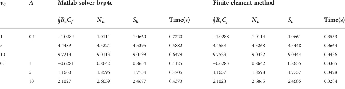
TABLE 1. Comparison of finite element method with Matlab solver bvp4c using $Gr=\mathit{1},Gm=\mathit{0.9},{\beta }_{\mathit{1}}=\mathit{0.3},{\beta }_{\mathit{2}}=\mathit{0.9},R_d=\mathit{0.1},P_r=\mathit{0.9},S_c=\mathit{0.9},\gamma =\mathit{0.1}$

TABLE 2

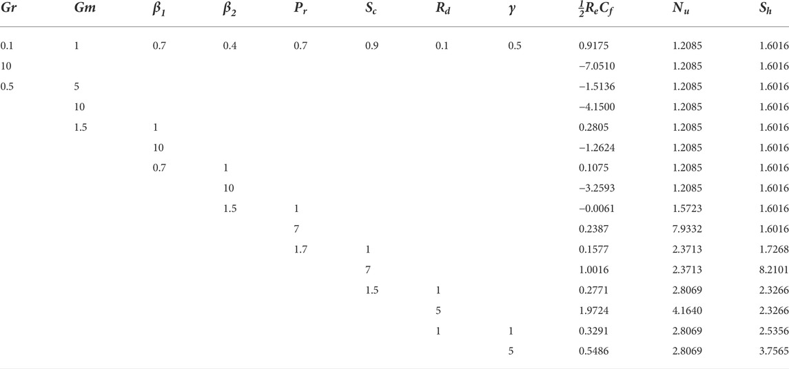
TABLE 2. By adjusting various dimensionless factors, we may obtain numerical values for the skin friction coefficient, the local Nusselt number, and the local Sherwood number as $A=\mathit{1},v_{\mathit{0}}=\mathit{1}$

Results and discussions

The modified finite element approach handles boundary value problems, which is very effective. To check the validity of the obtained results, a set of obtained non-dimensional boundary values problems is also solved by employing Matlab solver bvp4c. In implementing the modified finite element method, linear first-degree interpolation polynomials are considered to vanish when their second-order derivatives are found. But in the present application of the modified finite element method, weak formulations are constructed, which are obtained by finding the integration of parts to the strong formulations. So, in this manner, all derivatives that appear in the weak formulations are first order. So, one of the advantages of using weak formulations rather than strong formulations is to provide freedom for choosing linear interpolating polynomials. The second important advantage of using the present implementation of the modified finite element method is to provide faster integration based on the numerical Gauss Quadrature rule. Since exact analytical integration consumes time in the modified finite element method’s framework, numerical integration is carried out.

Figures 2–9 are drawn using the Matlab code of the modified finite element method. The impact of different involved parameters on velocity, temperature, and concentration profiles can be seen in these Figures 2–9. Figure 2 shows the impact of the Grashof number on the velocity profile. Velocity profile escalates by enhancing Grashof number in heat transfer. This happened due to an increment in the buoyancy force by rising values of Grashof number in heat transfer. The increased buoyancy force generates a force in the flow that augments the velocity profile. Figure 3 deliberates the impact of modified (Solutal) Grashof number on the velocity profile.

FIGURE 2

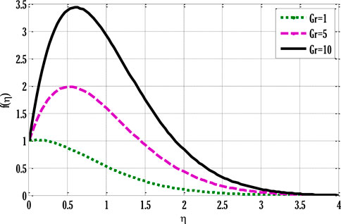
FIGURE 2. Effect of thermal Grashof number on velocity profile using $A=\mathit{1},v_{\mathit{0}}=\mathit{0.7},Gm=\mathit{1},{\beta }_{\mathit{1}}=\mathit{0.4},{\beta }_{\mathit{2}}=\mathit{0.4},P_r=\mathit{0.7},R_d=\mathit{1}.S_c=\mathit{0.9},\gamma =\mathit{0.7},N=\mathit{120}$.

FIGURE 3

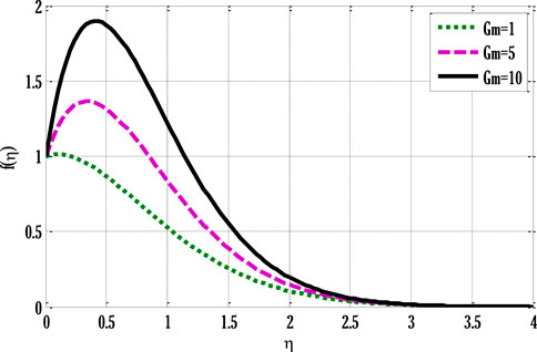
FIGURE 3. Effect of modified (solutal) Grashof number on velocity profile using $A=\mathit{1},v_{\mathit{0}}=\mathit{0.7},Gr=\mathit{1},{\beta }_{\mathit{1}}=\mathit{0.4},{\beta }_{\mathit{2}}=\mathit{0.4},P_r=\mathit{0.7},R_d=\mathit{1},S_c=\mathit{0.9},\gamma =\mathit{0.7},N=\mathit{120}$.

The velocity profile grows by rising modified Grashof number. Figure 4 shows the impact of non-linear thermal convection parameters on the velocity profile. Rising values of non-linear convection parameters enhance the velocity profile. Since increment in the non-linear thermal convection variable leads to an increase in temperature difference between the wall and ambient temperatures, the velocity profile escalates. Figure 5 deliberates the velocity profile by varying non-linear solutal convection variables. An increment in the non-linear solutal convection variable leads to growth in the velocity profile. A higher solutal variable leads to a rise in the concentration difference between wall and ambient concentrations. This increase in the concentration difference produces a rise in the velocity profile. Figure 6 shows the temperature profile by varying radiation parameters. Figure 6 shows that temperature grows by increment in the radiation parameter. The enhancement in the temperature profile results from rising surface heat flux that rises by incoming radiations, so the fluid temperature escalates. Figure 7 deliberates the impact of the Prandtl number on the temperature profile. The temperature de-escalates by growing values of the Prandtl number. It happens due to decay in the thermal diffusivity when the Prandtl number grows, leading to a fall in thermal conductivity and, subsequently, the temperature profile de-escalates. Figure 8 deliberates the impact of Schmidt number on concentration profile. Figure 8 shows that concentration decreases by enhancing the Schmidt number.

FIGURE 4

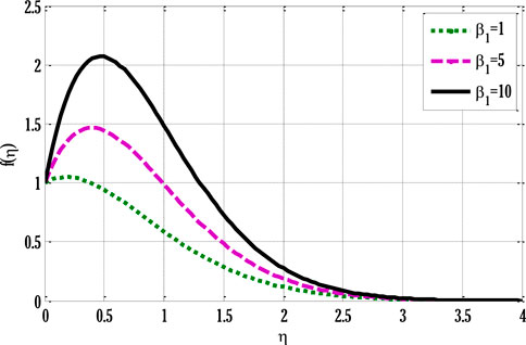
FIGURE 4. Effect of non-linear thermal convection parameter on velocity profile using $A=\mathit{1},v_{\mathit{0}}=\mathit{0.7},Gm=\mathit{1},Gr=\mathit{1},{\beta }_{\mathit{2}}=\mathit{0.4},P_r=\mathit{0.7},R_d=\mathit{1},S_c=\mathit{0.9},\gamma =\mathit{0.7},N=\mathit{120}$.

FIGURE 5

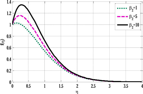
FIGURE 5. Effect of non-linear solutal convection parameter on velocity profile using $A=\mathit{1},v_{\mathit{0}}=\mathit{0.7},Gm=\mathit{1},{\beta }_{\mathit{1}}=\mathit{0.4},Gr=\mathit{1},P_r=\mathit{0.7},R_d=\mathit{1}.S_c=\mathit{0.9},\gamma =\mathit{0.7},N=\mathit{120}$.

FIGURE 6

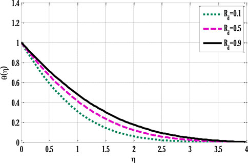
FIGURE 6. Effect of radiation parameter on temperature profile using $A=\mathit{1},v_{\mathit{0}}=\mathit{0.7},Gm=\mathit{1},{\beta }_{\mathit{1}}=\mathit{0.4},{\beta }_{\mathit{2}}=\mathit{0.4},P_r=\mathit{0.7},Gr=\mathit{1},S_c=\mathit{0.9},\gamma =\mathit{0.7},N=\mathit{120}$.

FIGURE 7

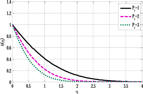
FIGURE 7. Effect of Prandtl number on temperature profile using $A=\mathit{1},v_{\mathit{0}}=\mathit{0.7},Gm=\mathit{1},{\beta }_{\mathit{1}}=\mathit{0.4},{\beta }_{\mathit{2}}=\mathit{0.4},R_d=\mathit{1},Gr=\mathit{1},S_c=\mathit{0.9},\gamma =\mathit{0.7},N=\mathit{120}$.

FIGURE 8

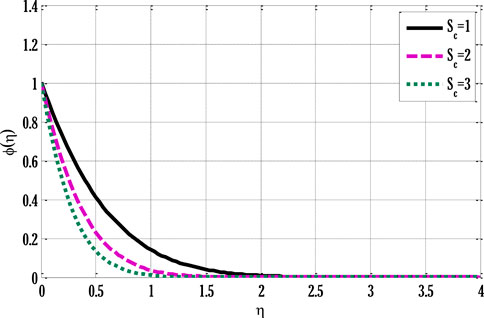
FIGURE 8. Effect of Schmidt number on concentration profile using $A=\mathit{1},v_{\mathit{0}}=\mathit{0.7},Gm=\mathit{1},{\beta }_{\mathit{1}}=\mathit{0.4},{\beta }_{\mathit{2}}=\mathit{0.4},Gr=\mathit{1},R_d=\mathit{1}.P_r=\mathit{0.7},\gamma =\mathit{0.7},N=\mathit{120}$.

The decrease in molecular diffusivity resulted in a slower concentration profile. Figure 9 displays the impact of reaction rate parameters on concentration profile. The concentration profile decreases by rising values of the reaction rate parameter. The decay in the concentration profile is the consequence of either a rising impurity level or an increase in making new substances. Figure 10 is drawn using software that can be used to solve a set of partial differential equations. This problem requires some inputs in the forms of partial differential equations, boundary conditions at the walls, and an additional non-linear source as a force is added. Its output can be seen in different types of graphs.

FIGURE 9

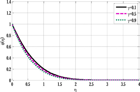
FIGURE 9. Effect of reaction rate parameter on concentration profile using $A=\mathit{1},v_{\mathit{0}}=\mathit{0.7},Gm=\mathit{1},{\beta }_{\mathit{1}}=\mathit{0.4},{\beta }_{\mathit{2}}=\mathit{0.4},Gr=\mathit{1},R_d=\mathit{1},P_r=\mathit{0.7},Sc=\mathit{0.9},N=\mathit{120}$.

FIGURE 10

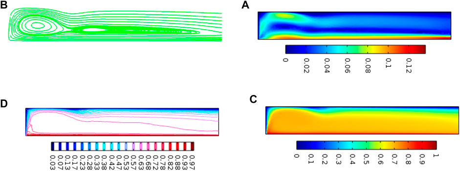
FIGURE 10. Surfaces for velocity, streamlines, temperature, and isothermal contours using non-linear thermal convection.

The values for the skin friction coefficient, the local Nusselt number, and the local Sherwood number are listed in Table 1. Skin friction coefficient decreases by increasing Grashof numbers in heat and mass transfer, non-linear thermal solutal convection parameters, and radiation parameters. An increase in thermal and solutal Grashof numbers produces a lower skin friction coefficient, and mathematically it is the consequence of escalation in slopes of tangents of the velocity profile at $\eta =0$ when velocity escalates and negative sign with $f^{\prime }\left(0\right)$ changes the increase of slopes of tangents to decrease in the slope of tangents. By increasing thermal and solutal Grashof number, the velocity of the flow grows due to a decrease in kinematic viscosity that leads to slower down friction at the wall and, therefore, skin friction coefficient decreases. It is also escalated by enhancing the Prandtl number, Schmidt number, and reaction rate parameters. The local Nusselt number is escalated by rising Prandtl number and radiation parameter. Increased conductive heat transport in the sheet due to increased radiation entrance increases the local Nusselt number. The Schmidt number and reaction rate parameters grow the local Sherwood number.

Conclusion

The mathematical model for the flow over the sheet has been modified by considering the effects of non-linear mixed convection. The linear and non-linear sets of PDEs were reduced to ordinary differential equations using similarity transformations. The dimensionless equations have been solved using the modified finite element method and Matlab solver bvp4c. The effect of different dimensionless parameters on velocity, temperature, and concentration profiles has been given in graphs. The main concluded results are described as

• Velocity profile escalated by rising values of non-linear thermal and solutal convection parameters.

• Temperature profile escalated and de-escalated by increment in radiation parameter and Prandtl number.

• The concentration profile was de-escalated by increasing the Schmidt number and reaction rate parameter.

• Skin friction coefficient de-escalated by growth in thermal and Grashof numbers.

Data availability statement

The original contributions presented in the study are included in the article/Supplementary Material, further inquiries can be directed to the corresponding author.

Author contributions

tConceptualization, YN; Funding acquisition, KA; Investigation, Software, Formal Analysis, Writing—review and editing, Methodology, and Writing—original draft, YN; Methodology, MA; Project administration, KA; Resources, KA; Supervision, MA; Visualization, KA; Writing—review and editing, MA. All authors have read and agreed to the published version of the manuscript.

Funding

The authors would like to acknowledge the support of Prince Sultan University for paying the Article Processing Charges (APC) of this publication.

Acknowledgments

The authors wish to express their gratitude to Prince Sultan University for facilitating the publication of this article through the Theoretical and Applied Sciences Lab.

Conflict of interest

The authors declare that the research was conducted in the absence of any commercial or financial relationships that could be construed as a potential conflict of interest.

Publisher’s note

All claims expressed in this article are solely those of the authors and do not necessarily represent those of their affiliated organizations, or those of the publisher, the editors and the reviewers. Any product that may be evaluated in this article, or claim that may be made by its manufacturer, is not guaranteed or endorsed by the publisher.

References

1. Hayat T, Naseem A, Farooq M, Alsaedi A. Unsteady MHD three-dimensional flow with viscous dissipation and Joule heating. Eur Phys J Plus (2013) 128:158. doi:10.1140/epjp/i2013-13158-1

CrossRef Full Text | Google Scholar

2. Mukhopadhyay S. MHD boundary layer flow and heat transfer over an exponentially stretching sheet embedded in a thermally stratified medium. Alexandria Eng J (2013) 52:259–65. doi:10.1016/j.aej.2013.02.003

CrossRef Full Text | Google Scholar

3. Bhattacharyya K, Vajravelu K. Stagnation-point flow and heat transfer over an exponentially shrinking sheet. Commun Nonlinear Sci Numer Simul (2012) 17:2728–34. doi:10.1016/j.cnsns.2011.11.011

CrossRef Full Text | Google Scholar

4. Elbashbeshy EMA, Emam TG, Abdelgaber KM. Effects of thermal radiation and magnetic field on unsteady mixed convection flow and heat transfer over an exponentially stretching surface with suction in the presence of internal heat generation/absorption. J Egypt Math Soc (2012) 20:215–22. doi:10.1016/j.joems.2012.08.016

CrossRef Full Text | Google Scholar

5. Bhattacharyya K, Mukhopadhyay S, Layek GC. Similarity solution of mixed convective boundary layer slip flow over a vertical plate. Ain Shams Eng J (2013) 4:299–305. doi:10.1016/j.asej.2012.09.003

CrossRef Full Text | Google Scholar

6. Mukhopadhyay S, Ishak A. Mixed convection flow along a stretching cylinder in a thermally stratified medium. J Appl Math (2012) 2012:1–8. doi:10.1155/2012/491695

CrossRef Full Text | Google Scholar

7. Hayat T, Ashraf MB, Alsulami HH, Alhuthali MS. Three-dimensional mixed convection flow of Viscoelastic fluid with thermal radiation and convective conditions. Plos ONE (2014) 9:e90038. doi:10.1371/journal.pone.0090038

PubMed Abstract | CrossRef Full Text | Google Scholar

8. Rashidi MM, Ashraf M, Rostami B, Rastegari MT, Bashir S. Mixed convection boundary-layer flow of a micro polar fluid towards a heated shrinking sheet by homotopy analysis method. Ther Sci (2013) 20. doi:10.2298/TSCI130212096R

CrossRef Full Text | Google Scholar

9. Hayat T, Khan MWA, Khan MI, Waqas M, Alsaedi A. Impact of chemical reaction in fully developed radiated mixed convective flow between two rotating disk. Physica B: Condensed Matter (2018) 538:138–49. doi:10.1016/j.physb.2018.01.068

CrossRef Full Text | Google Scholar

10. Hayat T, Qayyum S, Waqas M, Ahmed B. Influence of thermal radiation and chemical reaction in mixed convection stagnation point flow of Carreau fluid. Results Phys (2017) 7:4058–64. doi:10.1016/j.rinp.2017.10.018

CrossRef Full Text | Google Scholar

11. Ahmad S, Farooq M, Javed M, Anjum A. Double stratification effects in chemically reactive squeezed Sutterby fluid flow with thermal radiation and mixed convection. Results Phys (2018) 8:1250–9. doi:10.1016/j.rinp.2018.01.043

CrossRef Full Text | Google Scholar

12. Khan I, Khan M, Malik MY, Salahuddin T. Mixed convection flow of Eyring-Powell nanofluid over a cone and plate with chemical reactive species. Results Phys (2017) 7:3716–22. doi:10.1016/j.rinp.2017.08.042

CrossRef Full Text | Google Scholar

13. Maleque KA. Unsteady natural convection boundary layer flow with mass transfer and a binary chemical reaction. Br J Appl Sci Technol (2013) 3(1):131–49. doi:10.9734/bjast/2014/2265

CrossRef Full Text | Google Scholar

14. Abdul Maleque K. Effects of exothermic/endothermic chemical reactions with arrhenius activation energy on MHD free convection and mass transfer flow in presence of thermal radiation. J Thermodynamics (2013) 692516:11. doi:10.1155/2013/692516

CrossRef Full Text | Google Scholar

15. Maleque KA. Unsteady natural convection boundary layer heat and mass transfer flow with exothermic chemical reactions. J Pure Appl Math Adv Appl (2013) 9(1):17–41.

Google Scholar

16. Shehzad SA, Alsaedi A, Hayat T, Alhuthali MS. Thermophoresis particle deposition in mixed convection threedimensional radiative flow of an Oldroyd-B fluid. J Taiwan Inst Chem Eng (2014) 45:787–94. doi:10.1016/j.jtice.2013.08.022

CrossRef Full Text | Google Scholar

17. Rajput S, Verma AK, Bhattacharyya K, Chamkha AJ. Unsteady non-linear mixed convective flow of nanofluid over a wedge: Buongiorno model (2021). doi:10.1080/17455030.2021.1987586

CrossRef Full Text | Google Scholar

18. Aslani K-E, Mahabaleshwar US, Singh J, Sarris IE. Combined effect of radiation and inclined MHD flow of a micropolar fluid over a porous stretching/shrinking sheet with mass transpiration. Int J Appl Comput Math (2021) 7:60. doi:10.1007/s40819-021-00987-7

CrossRef Full Text | Google Scholar

19. Siddheshwar PG, Mahabaleswar US. Effects of radiation and heat source on MHD flow of a viscoelastic liquid and heat transfer over a stretching sheet. Int J Non-Linear Mech (2005) 40:807–20. doi:10.1016/j.ijnonlinmec.2004.04.006

CrossRef Full Text | Google Scholar

20. Shahzad A, Ali R, Khan M. On the exact solution for axisymmetric flow and heat transfer over a nonlinear radially stretching sheet. Chin Phys Lett (2012) 29(8):084705. doi:10.1088/0256-307x/29/8/084705

CrossRef Full Text | Google Scholar

21. Merkin JH. On dual solutions occurring in mixed convection in a porous medium. J Eng Math (1985) 20:171–9. doi:10.1007/bf00042775

CrossRef Full Text | Google Scholar

22. Benos LT, Polychronopoulos ND, Mahabaleshwar US, Lorenzini G, Sarris IE. Thermal and flow investigation of MHD natural convection in a nanofluid-saturated porous enclosure: An asymptotic analysis. J Therm Anal Calorim (2021) 143:751–65. doi:10.1007/s10973-019-09165-w

CrossRef Full Text | Google Scholar

23. Wang Y, Naveen Kumar R, Gouadria S, Helmi MM, Punith Gowda RJ, El-Zahar ER, et al. A three-dimensional flow of an Oldroyd-B liquid with magnetic field and radiation effects: An application of thermophoretic particle deposition. Int Commun Heat Mass Transfer (2022) 134:106007.

CrossRef Full Text | Google Scholar

24. Kumar RN, Jyothi AM, Alhumade H, Gowda RP, Alam MM, Ahmad I, et al. Impact of magnetic dipole on thermophoretic particle deposition in the flow of Maxwell fluid over a stretching sheet. J Mol Liquids (2021) 334:116494. doi:10.1016/j.molliq.2021.116494

CrossRef Full Text | Google Scholar

25. Punith Gowda RJ, Naveen Kumar R, Jyothi AM, Prasannakumara BC, Nisar KS. KKL correlation for simulation of nanofluid flow over a stretching sheet considering magnetic dipole and chemical reaction. ZAMM - J Appl Maths Mech/Z für Angew Mathematik Mechanik (2021) 101(11):e202000372.

CrossRef Full Text | Google Scholar

26. Madhukesh JK, Naveen Kumar R, Punith Gowda RJ, Prasannakumara BC, Ramesh GK, Ijaz Khan M, et al. Numerical simulation of aa7072-aa7075/waterbased hybrid nanofluid flow over a curved stretching sheet with Newtonian heating: A non-fourier heat flux model approach. J Mol Liquids (2021) 335:116103. doi:10.1016/j.molliq.2021.116103

CrossRef Full Text | Google Scholar

27. Nawaz Y, Arif MS. Modified class of explicit and enhanced stability region schemes: Application to mixed convection flow in a square cavity with a convective wall. Int J Numer Meth Fluids (2021) 93:1759–87. doi:10.1002/fld.4951

CrossRef Full Text | Google Scholar

28. Pasha AS, Nawaz Y, Arif SM. A third-order accurate in time method for boundary layer flow problems. Appl Numer Maths (2021) 161:13–26. doi:10.1016/j.apnum.2020.10.023

CrossRef Full Text | Google Scholar

29. Nawaz Y, Arif MS, Shatanawi W, Nazeer A. An explicit fourth-order compact numerical scheme for heat transfer of boundary layer flow. Energies (2021) 14(2):3396. doi:10.3390/en14123396

CrossRef Full Text | Google Scholar

30. Rosseland S. Astrophysik und atom-theoretische Grundlagen. New York: Springer (1931).

Google Scholar