 Hongling Qiu1
 Heng Liu
- 1School of Science, Guangxi Minzu University, Nanning, China
- 2School of Mathematics and Statistics, Xinyang Normal University, Xinyang, China
- 3School of Mathematics and Statistics, Anhui Normal University, Wuhu, China
This study investigates the adaptive fuzzy output feedback control of strict-feedback fractional-order chaotic systems with unmeasurable states and quantized input. First, the functional uncertainties are approximated by fuzzy logic systems (FLSs). Second, combining the FLS and the system output signal, an observer is constructed to estimate the unmeasurable states. A command filter is defined to cope with the “explosion of complexity” problem resulting from the repeated derivatives of virtual control inputs in each backstepping step. To compensate for quantization errors, a hyperbolic tangent function is introduced to transform the control signal, which can not only guarantee that the tracking error converges to an arbitrarily small region near the origin but also reduce the chattering phenomenon of the control input. In addition, the stability analysis is carried out relying on the fractional Lyapunov stability criterion such that all the signals keep bounded. Finally, a numerical simulation example is put forward to verify the effectiveness of our method.
1 Introduction
During the past few decades, fractional calculus has received increasing research interest because of its special properties that can be well used in system modeling, such as heredity and memory. After a long period of development, it has been a powerful mathematical instrument in the fields of bioengineering, physics, economics, medicine, and so on [1–4]. At the same time, many traditional calculus theories have been extended to the fractional calculus theory, especially the Mittag–Leffler stability theory [5]. As an extension of the Lyapunov stability theory, it plays an important role when designing the controller for fractional-order nonlinear systems (FONSs), including fractional-order chaotic systems (FOCSs).
Strict-feedback systems are a common form of chaotic systems, such as fractional-order Arneodo systems [6] and fractional-order Rossler systems [7]. One of the effective strategies to control these systems is the backstepping technique. However, virtual control inputs need to be repeatedly differentiated in each backstepping step, which will cause the “explosion of complexity” problem. Furthermore, different from the traditional calculus, the fractional order derivative of a composite function is a complicated infinite series that is hard to be calculated in practical engineering, which also increases the difficulty of designing controllers for strict-feedback FONSs. To this end, researchers have done special research and some interesting results have been achieved. For instance, in [8, 9], the fractional-order derivative of the virtual control input was regarded as an extra uncertain term and was approximated by fuzzy logic systems (FLSs), which can avoid the “explosion of complexity” problem; however, as the order of the system increases, the cumulative increase of fuzzy errors will affect the final control performance. To reduce the influence of fuzzy errors, an adaptive dynamic surface control was extended to FONSs in [10]. Moreover, a fractional-order command filter and an exact differentiator were introduced in [11, 12], respectively.
In addition, it is worth pointing out that in the aforementioned literature, a key assumption, i.e., the states must be measurable and should be satisfied, which is too demanding for practical engineering applications. Constrained by sensor technology or cost consumption, in most cases, only the system output signal is measurable directly, which means that the unknown states need to be estimated by developing an observer. In [13], the tracking control problem for incommensurate FONSs with input saturation was addressed via the observer-based backstepping algorithm. In [14], an observer was proposed for FONSs with unknown input gain based on the LMI technique. A sliding mode observer came up for FONSs with parameter uncertainties in [15]. However, there are still some limitations in these works: the system model of [13] is considered to be free of functional uncertainties or disturbances; the method of [14] is only applicable to system models that can be linearized; and a switch term is included in the observer structure appearing in [15], which will result in the chatting phenomenon. Some other interesting methods can be seen in [16–19]. For the observer design of the FONS, there is still a lot of work worth exploring.
On the other hand, because of limited-bandwidth communication channels and data transmission pressure, the control input signal must be quantized for some systems, such as digital control systems, hydraulic systems, and network systems [20–22]. A common type of quantizer is the sector-bounded quantizer, whose quantization errors satisfy the sector-bounded condition, including uniform quantizers, logarithmic quantizers, and hysteretic quantizers. In [23], a method that divides a sector-bounded quantizer into a linear segment and a nonlinear segment was discussed, which is the main idea of the quantized controller design. During the past few years, considerable results about quantized control for integer-order nonlinear systems have been achieved [24–27], and several important conclusions have been successfully extended to FONSs. For example, in [28], a Nussbaum function was used to study the fuzzy quantized control problem for uncertain FONSs with unknown control directions; in [29], a logarithmic quantizer was employed to achieve the synchronization control for fractional-order output-coupling neural networks; in [30], for a FONS with input quantization and actuator failures, an adaptive asymptotic tracking control strategy was proposed; in [31], an output-feedback quantized controller was designed for fractional-order neural networks described by Takagi–Sugeno fuzzy models; and in [32], the neural network-based quantized synchronization control for FOCSs was investigated. Nevertheless, it should be noted that the aforementioned literature treats the nonlinear part decomposed by the quantizer as an extra disturbance. How to better compensate for the quantization error in the design of the control input is still a matter of concern.
Inspired by the aforementioned discussion, this study investigates the adaptive fuzzy output feedback control problem for strict-feedback FOCSs subject to unmeasurable states and input quantization. The main contributions of this work are listed as follows. 1) Compared with the results presented in [13, 14], a broader class of FOCSs with functional uncertainties in each subsystem has been investigated. 2) Taking into account limited communication channels and data transmission pressure, a logarithmic quantizer is used to quantize the input signal, which has a better application value for actual engineering. 3) In comparison with the method of compensating for quantization errors in [24], a hyperbolic tangent function is introduced to transform the control signal in the controller design so that the disturbance derived from the nonlinear part of the quantizer is cleverly avoided and the chatting phenomenon is reduced. 4) Distinct from [28–32], all the states of the system model considered in this work are supposed to be unknown except the output signal.
The article is organised as follows. Some basic knowledge of fractional calculus and the problem description are provided in Section 2; Section 3 gives the details about the design of the observer and the controller; simulation results are presented in Section 4; and Section 5 summarizes the conclusion. In the following,
2 Preliminaries and Problem Description
2.1 Preliminaries
Definition 1 [33] The Caputo’s fractional derivative is defined as
where 0 < ϑ < 1.
Lemma 1 [34] Suppose that
Lemma 2 [10] Let
where a, b > 0 are constants. Then, there exists a constant t0 > 0 such that
holds for all t ≥ t0, where c0 > 1 is a constant.
Lemma 3 [11] The fractional-order command filter is defined as
where γ1 (0) = α(0) and γ2 (0) = 0. The function α(t) is the input signal that satisfies
2.2 Problem Description
Consider the following FOCS with a strict-feedback form:
where
Assumption 1 yd(t) and
Assumption 2 For
The logarithmic quantizer is characterized as follows:
where j = 1, 2, ⋯, umin > 0, ξ ∈ (0, 1), uj = ξ1−jumin,
3 Main Results
Since all the states of the system are unmeasurable except the output signal, it is essential to design an observer first.
3.1 Observer Design
Let
where
Remark 1. Since
which means that
where
where
where
where
Let
where
3.2 Controller Design
Based on the information derived from the observer, the final controller will be given via the backstepping algorithm in this part. The whole design process is divided into n steps.
Step 1: let e1(t) = x1(t) − yd(t), whose fractional order derivative can be expressed by
where α1(t) is the first virtual control input,
where γ1,1 (0) = α1 (0) and γ1,2 (0) = 0. In terms of Lemma 3, for any μ1 > 0, there exist β1 > 0 and ζ1 ∈ (0, 1] such that |γ1,1(t) − α1(t)| ≤ μ1 for all t > 0.
Choose the virtual control input α1(t) to be
where c1 > 0 is a design parameter. Substituting (21) into (19), one obtains
Let
where r1, a1 > 0 are design parameters.
Construct a Lyapunov function as
Utilizing Young’s inequality, one has
where η1 > 0 is a constant. Hence, one gets
Step i (i = 2, … , n − 1): similar to the previous step, the ϑ-th derivative of ei(t) is
where αi(t) is the ith virtual control input,
where γi,1 (0) = αi (0) and γi,2 (0) = 0. Similarly, for any μi > 0, there exist βi > 0 and ζi ∈ (0, 1] such that |γi,1(t) − αi(t)| ≤ μi for all t > 0. We choose
where ci > 0 is a design parameter. It follows from (27) and (29) that
We design the adaptation law
where ri, ai are positive design parameters. We select the Lyapunov function as
Because of the property that
where ηi > 0 is a constant. Substituting (33) into (32), one obtains
Step n: the ϑ-th derivative of en(t) is given by
The controller u(t) is designed as
where cn, γ > 0 are two design parameters and χ > umin is a constant. Let the adaptation law of
where rn, an > 0 are design parameters. Defining a Lyapunov function as
Considering the term
where δ1 = 0.2785γ(1 − ϱ) and δ2 = 0.2785γ(2 − ϱ). Substituting (39) into (38), one obtains
Similar to (33), one has
where ηn > 0 is a constant. Then,
Therefore, based on the aforementioned analysis, the stability analysis can be summarized as the following theorem.
Theorem 1 Consider system (6) under Assumptions 1–2. The observer and quantizer are (15) and (8), respectively. The virtual control inputs are given by (21) and (29), and the corresponding filters are defined as (20) and (28). Consequently, the controller (36) with the parameter adaptation laws (23) (31), and (37) can guarantee that the tracking error e1(t) and the estimation error
Proof. Define a Lyapunov function as
By means of Eq. 26, Eq. 34, and Eq. 42, one has
We define
From Eq. 17, one has
Using Young’s inequality, one has
It follows from Eq. 46 and Eq. 47 that
Let V(t) = V1(t) + V2(t), then from Eq. 44 and Eq. 48, one has
Setting the parameters to ensure
in which
Remark 2 According to the principle of the backstepping algorithm, the role of αi(t) is to act as the controller of the ith subsystem, and
Remark 3 The advantages of the filter (28) can not only avoid the “explosion of complexity” problem, but also release the condition of Assumption 2 in [37] (the knowledge of
Remark 4 It can be seen from the definitions of a and b in (50) that the range of
Remark 5 It is worth noting that the property (9) is possessed by all sector-bounded quantizers, which means that our method is valid for other forms of quantizers, such as hysteretic quantizers and uniform quantizers.
Remark 6 The scheme of designing a variable structure-quantized controller introduced in [24] can also be applied to our work. The main idea is based on the following properties of (8):
Using the method of [24], the controller u(t) can be designed as
Then, according to (51), one has
Substituting (53) into (38), one has
Then, (42) can be rewritten as
The following analysis is the same as the proof of theorem 1. The controller (52) is valid for controlling system (6), which will be demonstrated in the simulation part; however, because there is a discontinuous function sign (⋅) in (52), a serious chattering phenomenon will occur.
4 Simulation Results
In this section, a simulation example is provided to show the performance of the proposed method, and this example will show the superiority of our method in comparison with [24].
We consider the fractional-order Chua–Hartley’s chaotic system
where
The parameter selections are chosen as follows. First, we set c1 = 4 and c2 = 4 for the virtual inputs in (21) and (29), respectively; second, we set c3 = 5, χ = 0.15 and γ = 1.5 for the controller in (36); third, we set K = [k1, k2, k3] = [10, 30, 200] and
The simulation result of the tracking trajectory is presented in Figure 1A. It is clear that our method achieves a better control effect. The real states of system 56) and the estimated states are shown in Figures 1B–D. However, because of the existence of fuzzy errors, the observer curves and the real state curves cannot be completely consistent. The actual control input and the corresponding quantized input are displayed in Figure 2A and Figure 2B, respectively.
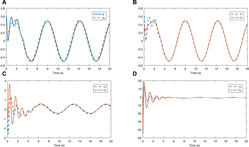
FIGURE 1. (A) Tracking performance of the output y(t). (B) x1(t) and
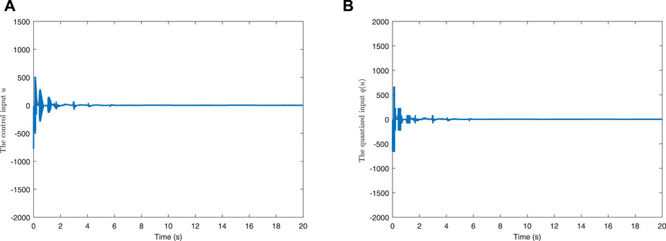
FIGURE 2. (A) Control input u(t). (B) Quantized input q (u(t)).
To reflect the superiority of our approach, the actual control input and the corresponding quantized input by using the method of [24] are depicted in Figure 3A and Figure 3B, respectively, and the performance comparison between the two methods is shown in Figure 4. It can be seen that under the same parameter-setting conditions, compared with [24], not only is the control effect almost the same, but also the ability to save the control energy and reduce the chattering has been greatly improved.
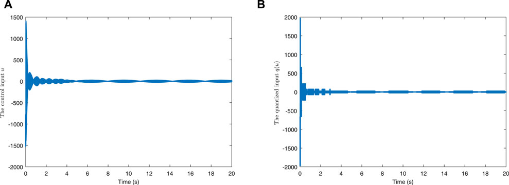
FIGURE 3. (A) Control input u(t). (B) Quantized input q (u(t)).
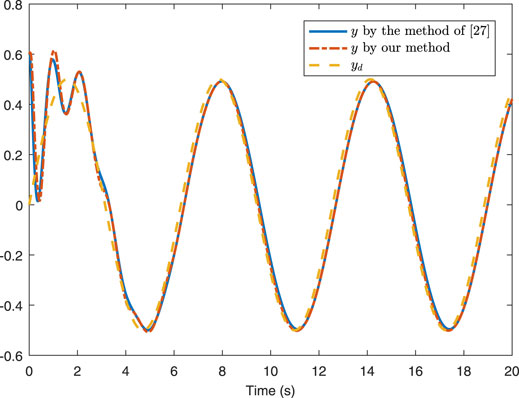
FIGURE 4. Comparative results between our approach and the method proposed by [24].
Remark 7 In this simulation, the step size is selected as h = 0.001s. In fact, since the use of the hyperbolic tangent function instead of the function sign (⋅), the input of the controller is continuous, so the chattering phenomenon does not exist theoretically. If the step size is selected as h = 0.0001s, and γ is increased, the chatting will be reduced to some extent.
5 Conclusion
The tracking control problem for strict-feedback FONSs with unknown states and functional uncertainties has been addressed in this study via the backstepping algorithm. To decrease the data transmission pressure and make use of communication channel effectively, a logarithmic quantizer is considered in the controller design. With the help of the fractional Lyapunov stability criterion, the tracking error and the estimation error converge to a small region near the origin and the boundedness of all the signals of the controlled plant is guaranteed. However, on the one hand, because of the existence of fuzzy errors, the control performance may be affected. On the other hand, the chattering phenomenon still exists. Hence, further work will focus on how to improve the recognition accuracy of FLSs and eliminate the chattering.
Data Availability Statement
The original contributions presented in the study are included in the article/Supplementary Material, further inquiries can be directed to the corresponding author.
Author Contributions
All authors listed have made a substantial, direct, and intellectual contribution to the work and approved it for publication.
Funding
This work is supported by the National Natural Science Foundation of China under Grant No. 12001012 and the Natural Science Foundation of Anhui Province of China under Grant No. 2008085QA10.
Conflict of Interest
The authors declare that the research was conducted in the absence of any commercial or financial relationships that could be construed as a potential conflict of interest.
Publisher’s Note
All claims expressed in this article are solely those of the authors and do not necessarily represent those of their affiliated organizations, or those of the publisher, the editors, and the reviewers. Any product that may be evaluated in this article, or claim that may be made by its manufacturer, is not guaranteed or endorsed by the publisher.
References
1. Magin RL. Fractional Calculus Models of Complex Dynamics in Biological Tissues. Comput Mathematics Appl (2010) 59(5):1586–93. doi:10.1016/j.camwa.2009.08.039
2. Ali Akbar M, Ali NHM, Mohd. Ali N, Tarikul Islam M. Multiple Closed Form Solutions to Some Fractional Order Nonlinear Evolution Equations in Physics and Plasma Physics. AIMS Mathematics (2019) 4(3):397–411. doi:10.3934/math.2019.3.397
3. Yousefpour A, Jahanshahi H, Munoz-Pacheco JM, Bekiros S, Wei Z. A Fractional-Order Hyper-Chaotic Economic System with Transient Chaos. Chaos, Solitons & Fractals (2020) 130:109400. doi:10.1016/j.chaos.2019.109400
4. Kumar D, Singh J. Fractional Calculus in Medical and Health Science. Boca Raton, FL: CRC Press (2020).
5. Li Y, Chen Y, Podlubny I. Mittag-Leffler Stability of Fractional Order Nonlinear Dynamic Systems. Automatica (2009) 45(8):1965–9. doi:10.1016/j.automatica.2009.04.003
6. Lu JG. Chaotic Dynamics and Synchronization of Fractional-Order Arneodo's Systems. Chaos, Solitons & Fractals (2005) 26(4):1125–33. doi:10.1016/j.chaos.2005.02.023
7. Shukla MK, Sharma BB. Backstepping Based Stabilization and Synchronization of a Class of Fractional Order Chaotic Systems. Chaos, Solitons & Fractals (2017) 102:274–84. doi:10.1016/j.chaos.2017.05.015
8. Liu H, Pan Y, Li S, Chen Y. Adaptive Fuzzy Backstepping Control of Fractional-Order Nonlinear Systems. IEEE Trans Syst Man Cybern, Syst (2017) 47(8):2209–17. doi:10.1109/tsmc.2016.2640950
9. Ha S, Liu H, Li S, Liu A. Backstepping-based Adaptive Fuzzy Synchronization Control for a Class of Fractional-Order Chaotic Systems with Input Saturation. Int J Fuzzy Syst (2019) 21(5):1571–84. doi:10.1007/s40815-019-00663-5
10. Liu H, Pan Y, Cao J. Composite Learning Adaptive Dynamic Surface Control of Fractional-Order Nonlinear Systems. IEEE Trans Cybern (2020) 50(6):2557–67. doi:10.1109/TCYB.2019.2938754
11. Ha S, Chen L, Liu H. Command Filtered Adaptive Neural Network Synchronization Control of Fractional-Order Chaotic Systems Subject to Unknown Dead Zones. J Franklin Inst (2021) 358(7):3376–402. doi:10.1016/j.jfranklin.2021.02.012
12. Wei Y, Du B, Cheng S, Wang Y. Fractional Order Systems Time-Optimal Control and its Application. J Optim Theor Appl (2017) 174(1):122–38. doi:10.1007/s10957-015-0851-4
13. Sheng D, Wei Y, Cheng S, Wang Y. Observer-based Adaptive Backstepping Control for Fractional Order Systems with Input Saturation. ISA Trans (2018) 82:18–29. doi:10.1016/j.isatra.2017.06.021
14. Kong S, Saif M, Liu B. Observer Design for a Class of Nonlinear Fractional-Order Systems with Unknown Input. J Franklin Inst (2017) 354(13):5503–18. doi:10.1016/j.jfranklin.2017.06.011
15. Zhong F, Li H, Zhong S. State Estimation Based on Fractional Order Sliding Mode Observer Method for a Class of Uncertain Fractional-Order Nonlinear Systems. Signal Process. (2016) 127:168–84. doi:10.1016/j.sigpro.2016.02.022
16. Phat V, Niamsup P, Thuan MV. A New Design Method for Observer-Based Control of Nonlinear Fractional-Order Systems with Time-Variable Delay. Eur J Control (2020) 56:124–31. doi:10.1016/j.ejcon.2020.02.005
17. Yen DTH, Huong DC. Functional Interval Observers for Nonlinear Fractional-Order Systems with Time-Varying Delays and Disturbances. Proc Inst Mech Eng J Syst Control Eng (2021) 235(4):550–62. doi:10.1177/0959651820945828
18. Kammogne AST, Kountchou MN, Kengne R, Azar AT, Fotsin HB, Ouagni STM. Polynomial Robust Observer Implementation Based Passive Synchronization of Nonlinear Fractional-Order Systems with Structural Disturbances. Front Inform Technol Electron Eng (2020) 21(9):1369–86. doi:10.1631/fitee.1900430
19. Zhan T, Tian J, Ma S. Full-order and Reduced-Order Observer Design for One-Sided Lipschitz Nonlinear Fractional Order Systems with Unknown Input. Int J Control Autom Syst (2018) 16(5):2146–56. doi:10.1007/s12555-017-0684-z
20. Cittanti D, Gregorio M, Mandrile F, Bojoi R. Full Digital Control of an All-Si On-Board Charger Operating in Discontinuous Conduction Mode. Electronics (2021) 10(2):203. doi:10.3390/electronics10020203
21. Chaker MA, Triki A. The Branching Redesign Technique Used for Upgrading Steel-Pipes-Based Hydraulic Systems: Re-examined. J Press Vessel Technology (2021) 143(3):031302. doi:10.1115/1.4047829
22. Choi YH, Yoo SJ. Neural-networks-based Adaptive Quantized Feedback Tracking of Uncertain Nonlinear Strict-Feedback Systems with Unknown Time Delays. J Franklin Inst (2020) 357(15):10691–715. doi:10.1016/j.jfranklin.2020.08.046
23. Zhou J, Wen C, Yang G. Adaptive Backstepping Stabilization of Nonlinear Uncertain Systems with Quantized Input Signal. IEEE Trans Automatic Control (2013) 59(2):460–4. doi:10.1109/TAC.2013.2270870
24. Aslmostafa E, Ghaemi S, Badamchizadeh MA, Ghiasi AR. Adaptive Backstepping Quantized Control for a Class of Unknown Nonlinear Systems. ISA Trans (2021). doi:10.1016/j.isatra.2021.06.009
25. Abdelrahim M, Dolk VS, Heemels WPMH. Event-triggered Quantized Control for Input-To-State Stabilization of Linear Systems with Distributed Output Sensors. IEEE Trans Automat Contr (2019) 64(12):4952–67. doi:10.1109/tac.2019.2900338
26. Zhou J, Wen C, Wang W, Yang F. Adaptive Backstepping Control of Nonlinear Uncertain Systems with Quantized States. IEEE Trans Automat Contr (2019) 64(11):4756–63. doi:10.1109/tac.2019.2906931
27. Yoo SJ, Park BS. Quantized-states-based Adaptive Control against Unknown Slippage Effects of Uncertain mobile Robots with Input and State Quantization. Nonlinear Anal Hybrid Syst (2021) 42:101077. doi:10.1016/j.nahs.2021.101077
28. Song S, Park JH, Zhang B, Song X, Zhang Z. Adaptive Command Filtered Neuro-Fuzzy Control Design for Fractional-Order Nonlinear Systems with Unknown Control Directions and Input Quantization. IEEE Transactions on Systems, Man, and Cybernetics: Systems (2020) 51(11):7238–7249. doi:10.1109/TSMC.2020.2967425
29. Bao H, Park JH, Cao J. Adaptive Synchronization of Fractional-Order Output-Coupling Neural Networks via Quantized Output Control. IEEE Transactions on Neural Networks and Learning Systems (2020) 32(7):3230–3239. doi:10.1109/TNNLS.2020.3013619
30. Sabeti F, Shahrokhi M, Moradvandi A. Adaptive Asymptotic Tracking Control of Uncertain Fractional-Order Nonlinear Systems with Unknown Quantized Input and Control Directions Subject to Actuator Failures. J Vibration Control (2021) 10775463211017718. doi:10.1177/10775463211017718
31. Karthick SA, Sakthivel R, Ma YK, Mohanapriya S, Leelamani A. Disturbance Rejection of Fractional-Order T-S Fuzzy Neural Networks Based on Quantized Dynamic Output Feedback Controller. Appl Mathematics Comput (2019) 361:846–57. doi:10.1016/j.amc.2019.06.029
32. Zouari F, Boulkroune A, Ibeas A. Neural Adaptive Quantized Output-Feedback Control-Based Synchronization of Uncertain Time-Delay Incommensurate Fractional-Order Chaotic Systems with Input Nonlinearities. Neurocomputing (2017) 237:200–25. doi:10.1016/j.neucom.2016.11.036
33. Podlubny I. Fractional Differential Equations: an Introduction to Fractional Derivatives, Fractional Differential Equations, to Methods of Their Solution and Some of Their Applications. Elsevier (1998).
34. Dai H, Chen W. New Power Law Inequalities for Fractional Derivative and Stability Analysis of Fractional Order Systems. Nonlinear Dyn (2017) 87(3):1531–42. doi:10.1007/s11071-016-3131-4
35. Wang L-X. Adaptive Fuzzy Systems and Control: Design and Stability Analysis. Upper Saddle River, NJ: Prentice-Hall (1994).
36. Jiang X, Mu X, Hu Z. Decentralized Adaptive Fuzzy Tracking Control for a Class of Nonlinear Uncertain Interconnected Systems with Multiple Faults and Denial-Of-Service Attack. IEEE Trans Fuzzy Syst (2020) 29(10):3130–41. doi:10.1109/TFUZZ.2020.3013700
Keywords: fractional-order chaotic system, fuzzy logic system, state observer, input quantization, backstepping
Citation: Qiu H, Huang C, Tian H and Liu H (2022) Observer-Based Adaptive Fuzzy Output Feedback Control of Fractional-Order Chaotic Systems With Input Quantization. Front. Phys. 10:882759. doi: 10.3389/fphy.2022.882759
Received: 24 February 2022; Accepted: 16 March 2022;
Published: 27 April 2022.
Edited by:
Qiang Lai, East China Jiaotong University, ChinaReviewed by:
Faisal Mehmood, Institute of Space Technology, PakistanFangyi You, Huaqiao University, China
Copyright © 2022 Qiu, Huang, Tian and Liu. This is an open-access article distributed under the terms of the Creative Commons Attribution License (CC BY). The use, distribution or reproduction in other forums is permitted, provided the original author(s) and the copyright owner(s) are credited and that the original publication in this journal is cited, in accordance with accepted academic practice. No use, distribution or reproduction is permitted which does not comply with these terms.
*Correspondence: Heng Liu, bGl1aGVuZzEyMkBnbWFpbC5jb20=