The coupled Boussinesq equation and its Darboux transformation on the time–space scale

Gel’fand-Dikii (GD) formalism is an approach for generating integrable systems in terms of fractional powers of the δ differential operator. In this paper, it extends the GD formalism associated with the third-order δ differential operator L to the time scale. Then, the coupled Boussinesq equation on the time–space scale is given by taking special values, and it can be reduced on different time–space scales. Moreover, the exact solutions of the coupled Boussinesq equation on the time–space scale and the classical Boussinesq equation are constructed via employing the extensions of the Darboux theorem and Crum theorem on the time scale.

1 Introduction

There are many methods to produce soliton equations, such as the Ablowitz–Kaup–Newel–Segur (AKNS) method [1], Ablowitz–Ladik (AL) method [2], and GD formalism [3]. Compared with the other two methods, the difference of GD formalism is that differential operators, shift operators, and their inverses are regarded as essential tools to generate integrable systems. In this formalism, arbitrary Lax pairs can be constructed from the calculation of fractional powers of the operator L [4]. In addition, it is also quite significant in studying the symmetries, bi-Hamiltonian formulations, and construction of recursive operators for nonlinear PDE [5–7].

Nevertheless, earlier studies mostly centered on continuous systems or discrete systems. Since there are some complex problems that can only be solved exactly when considering the parallel analysis of continuous and discrete cases, the time scale was initiated by Stefan Hilger in 1988 [8–10]. Recently, soliton equations on time scales have been studied widely [11–14]. Agarwal et al. defined hyperbolic functions on the time scale to solve evolution equations [15]. Gürses et al. extended the GD formalism on the time scale to obtain more universal integrable nonlinear dynamic equations and generated integrable equations in terms of integers $\mathbb{Z}$ and q-numbers particularly. On this basis, the Δ-Burgers hierarchy and its recursion operator were derived by taking appropriate δ differential operators [7]. Ahlbrandt et al. investigated the Hamiltonian system on the time scale and its symplectic flow properties [16].

Darboux theorem was first proposed by Darboux in 1882 from the eigenfunction of the Schrödinger equation and the covariant transformation of potential and applied to surface theory [17]. In 1995, Crum obtained a popularization of the Darboux theorem via a recurrent relation from the N-fold Darboux transformation [18]. The notable merit of DT (Darboux transformation) is that solutions of the soliton equation may be obtained by means of finite iteration, which results it in a research focus of integrable systems in continuous or discrete form [19–23]. A Lax pair for the modified Boussinesq equation and its DT was derived by Geng [24]. Nimmo constructed the DT for the discrete KP equation and reduced to the discrete BKP equation resulting from an invariance of the binary transformation [25]. At present, the DT has been considered on the time scale, and several research results have been acquired. Hovhannisyan et al. obtained a solution of the KdV equation hierarchy from extensions of the Darboux theorem and Crum theorem on the time scale calculus [13]. By using gauge transformation, Dong et al. obtained the DT of the Gerdjikov–Ivanov equation on the time–space scale [26]. However, the DT of integrable systems has still rarely been studied under the unified analysis of continuous systems and discrete systems.

The Boussinesq equation is an important soliton equation [27–29], alongside other important research achievements in physics and mathematics such as one-dimensional nonlinear lattice waves [30, 31], vibrations in a nonlinear string [27], and ion sound waves in plasma [32]. A normative approach was presented to obtain the DT for the classical Boussinesq system by Zhang et al. [33]. In [34], the new solutions of the Boussinesq–Burgers equation were achieved via applying a DT with multi-parameters [34]. In order to better promote the research of the Boussinesq equation on the time scale, the coupled Boussinesq equation and its exact solution will be obtained on the time–space scale by extending the GD formalism and Darboux theorem to the time scale in this paper.

This paper is organized as follows. In Section 2, through employing the GD formalism associated with the third-order δ differential operator L, the coupled Boussinesq equation on the time–space scale is produced from its spectral problem. Section 3 presents the exact solutions of the coupled Boussinesq equation on the time–space scale, and the single-soliton solution of the classical Boussinesq equation is achieved on the special time scale $\mathbb{R}$. The last section is the conclusion.

2 Coupled Boussinesq equation on the time–space scale

In this section, taking special values, we will establish the coupled Boussinesq equation on the time–space scale from the extension for GD formalism on the time scale. Primarily, we will introduce several notions connected to the time scale [8, 9, 35].

Definition 1. Let $\mathbb{T}$ be a time scale. For $s\in \mathbb{T}$, forward and backward jump operators ξ, ζ: $\mathbb{T}\to \mathbb{T}$ are specified as

$\xi \left(s\right)=\inf \left\{x\in \mathbb{T}:x>s\right\},\zeta \left(s\right)=\sup \left\{x\in \mathbb{T}:x<s\right\}.(1)$

Definition 2. Forward and backward jump distance functions μ, ν: $\mathbb{T}\to [0,+\infty )$ are specified as

$\mu \left(s\right)=\xi \left(s\right)-s,\nu \left(s\right)=s-\zeta \left(s\right),(2)$

which are also called graininess functions.

Lemma 1. When $\mathbb{T}=\mathbb{R}$, $\mathbb{T}=\mathbb{Z}$, forward jump operators and graininess functions become

$\begin{array}{cc}\hfill \xi \left(s\right)& =\inf \left(s,-\infty \right)=s,\xi \left(s\right)=\inf \left\{x+1,x+2,\cdots \right\}=x+1,\hfill \\ \hfill \mu \left(s\right)& =\xi \left(s\right)-s=0,\mu \left(s\right)=\xi \left(s\right)-s=1,\hfill \end{array}(3)$

respectively.

Theorem 1. Let ${\mathbb{T}}^k$ represent Hilger’s truncated set which is composed of $\mathbb{T}$ removing the largest left-scattered point in $\mathbb{T}$, and $f:\mathbb{T}\to \mathbb{R},s\in {\mathbb{T}}^k$,(1) when f is Δ differentiable at s, f is continuous at s;(2) when f is continuous at s and s is right-scattered, f is Δ differentiable at s

$f^{\left(s\right)}\left(s\right)=\frac{f\left(\xi \left(s\right)\right)-f\left(s\right)}{\mu \left(s\right)};$

(3) when s is right-dense, f is Δ differentiable at s and the limit

$\underset{y\to s}{\lim }\frac{f\left(s\right)-f\left(y\right)}{s-y}$

exists as a finite number. In this case, f^(s)(s) is equal to this limit;(4) when f is Δ differentiable at s,

$f\left(\xi \left(s\right)\right)≔f^{\xi }\left(s\right)=f\left(s\right)+\mu \left(s\right)f^{\left(s\right)}\left(s\right).$

Remark: when $\mathbb{T}=\mathbb{R}$, $\mathbb{T}=h\mathbb{Z}$, the Δ − derivative f^(s)(s) in (2) becomes

$\begin{array}{cc}\hfill f^{\left(s\right)}\left(s\right)& =f_s\left(s\right),\hfill \\ \hfill f^{\left(s\right)}\left(s\right)& =\frac{f\left(s+h\right)-f\left(s\right)}{h}\hfill \\ \hfill & =\frac{Ef-f}{h},\hfill \end{array}$

where E is the shift operator.Afterward, the general integrable nonlinear evolution equations on the time–space scale are generated via considering Theorem 2 and Theorem 3 [7].

Theorem 2. Let the Nth-order δ differential operator

$L=u_N{\delta }^N+u_{N-1}{\delta }^{N-1}+u_{N-2}{\delta }^{N-2}+\cdots +u_0,(4)$

where u_j (j = 0, …, N) are Δ-smooth functions with the time variable(t) and space variable(s). Here, the time variable is taken as continuous. By using the Lax equation

$\frac{\mathrm{d}L}{\mathrm{d}t}=\left[A,L\right],A={\left(L^{\frac{n}{N}}\right)}_{⩾0},n=\mathrm{1,2},\dots (5)$

hierarchies of integrable nonlinear evolution equations are produced, where n is a positive integer not divisible by N.

Theorem 3. Let

$L^{\frac{1}{3}}=a_1\delta +a_0+a_{-1}{\delta }^{-1}+a_{-2}{\delta }^{-2}+\cdots ,$

then, through employing the Gel’fand-Dikii formalism on the time scale, the operator A is obtained:

$A={\left(L^{\frac{2}{3}}\right)}_{\ge 0}=a_1{a}_1^{\xi }{\delta }^2+\left(a_1{a}_1^{\left(s\right)}+a_1{a}_0^{\xi }+a_1{a}_0\right)\delta +a_1{a}_0^{\left(s\right)}+a_1{a}_{-1}^{\xi }+a_0^2+a_{-1}{a}_1^{{\xi }^{-1}}.(6)$

When N = 3, Eq. 4 becomes

$L=u_3{\delta }^3+u_2{\delta }^2+u_1\delta +u_0.(7)$

Then, by substituting Eqs. 6, 7 into Eq. 5, we get

$\frac{dL}{dt}=\left[{\left(L^{\frac{2}{3}}\right)}_{\ge 0},L\right],(8)$

and the following equations

$a_1{a}_1^{\xi }{u}_3^{\xi \xi }-{\left(a_1{a}_1^{\xi }\right)}^{\xi \xi \xi }{u}_3=0,(9)$

$a_1{a}_1^{\xi }\left(u_3^{\left(s\right)\xi }+u_3^{\xi \left(s\right)}\right)-u_3{b}_2+a_1{a}_1^{\xi }{u}_2^{\xi \xi \xi }-u_2{\left(a_1{a}_1^{\xi }\right)}^{\xi \xi }+b_1{u}_3^{\xi }-u_3{b}_1^{\xi \xi \xi }=0,(10)$

$a_1{a}_1^{\xi }{u}_3^{\left(ss\right)}+a_1{a}_1^{\xi }{u}_1^{\xi \xi }-u_1{\left(a_1{a}_1^{\xi }\right)}^{\xi }+b_1{u}_3^{\left(s\right)}+b_1{u}_2^{\xi }-u_2{b}_1^{\xi \xi }-u_3{b}_3+u_3{b}_4=u_{3t},(11)$

$\begin{array}{cc}\hfill & u_1^{\xi \left(s\right)}+u_1^{\left(s\right)\xi }-u_3{\left(a_1{a}_1^{\xi }\right)}^{\left(sss\right)}-u_1{\left(a_1{a}_1^{\xi }\right)}^{\left(s\right)}+a_1{a}_1^{\xi }\left(u_2^{\left(ss\right)}+u_0^{\xi \xi }-u_0\right)\hfill \\ \hfill & +b_1{u}_2^{\left(s\right)}+b_1{u}_1^{\xi }-u_1{b}_1^{\xi }-u_2\left[{\left(a_1{a}_1^{\xi }\right)}^{\left(ss\right)}+b_1^{\left(s\right)\xi }+b_1^{\xi \left(s\right)}\right]-u_3{b}_5+u_2{b}_6=u_{2t},\hfill \end{array}(12)$

$a_1{a}_1^{\xi }\left(u_1^{\left(ss\right)}+u_0^{\xi \left(s\right)}+u_0^{\left(s\right)\xi }\right)+b_1{u}_1^{\left(s\right)}-u_1{b}_1^{\left(s\right)}+b_1{u}_0^{\xi }-u_0{b}_1-u_3{b}_7-u_2{b}_8+u_1{b}_9=u_{1t},(13)$

$a_1{a}_1^{\xi }{u}_0^{\left(ss\right)}+b_1{u}_0^{\left(s\right)}-u_3{b}_{10}^{\left(sss\right)}-u_2{b}_{10}^{\left(ss\right)}-u_1{b}_{10}^{\left(s\right)}=u_{0t}.(14)$

where

$\begin{array}{cc}\hfill b_1& =a_1{a}_1^{\left(s\right)}+a_1{a}_0^{\xi }+a_1{a}_0,\hfill \\ \hfill b_2& ={\left(a_1{a}_1^{\xi }\right)}^{\xi \xi \left(s\right)}+{\left(a_1{a}_1^{\xi }\right)}^{\xi \left(s\right)\xi }+{\left(a_1{a}_1^{\xi }\right)}^{\left(s\right)\xi \xi },\hfill \\ \hfill b_3& ={\left(a_1{a}_1^{\xi }\right)}^{\left(ss\right)p}+{\left(a_1{a}_1^{\xi }\right)}^{\left(s\right)\xi \left(s\right)}+{\left(a_1{a}_1^{\xi }\right)}^{\xi \left(ss\right)}+b_1^{\xi \xi \left(s\right)}+b_1^{\xi \left(s\right)\xi }+b_1^{\left(s\right)\xi \xi },\hfill \\ \hfill b_4& =a_1{a}_0^{\left(s\right)}-{\left(a_1{a}_0^{\left(s\right)}\right)}^{\xi \xi \xi }+a_1{a}_{-1}^{\left(s\right)}-{\left(a_1{a}_{-1}^{\left(s\right)}\right)}^{\xi \xi \xi }+a_{-1}{a}_1^{\xi -1}-{\left(a_{-1}{a}_{-1}^{\xi -1}\right)}^{\xi \xi \xi }\hfill \\ \hfill & +a_0^2-a_0^{\xi \xi \xi },\hfill \end{array}$

$\begin{array}{ll}\hfill b_5& ={\left(a_1{a}_0^{\left(s\right)}\right)}^{\left(s\right)\xi \xi }+{\left(a_1{a}_0^{\left(s\right)}\right)}^{\xi \xi \left(s\right)}+{\left(a_1{a}_0^{\left(s\right)}\right)}^{\xi \left(s\right)\xi }+b_1^{\left(ss\right)\xi }+b_1^{\left(s\right)\xi \left(s\right)}+b_1^{\xi \left(ss\right)}\hfill \\ \hfill & +{\left(a_1{a}_{-1}^{\xi }\right)}^{\xi \xi \left(s\right)}+{\left(a_1{a}_{-1}^{\xi }\right)}^{\xi \left(s\right)\xi }+{\left(a_1{a}_{-1}^{\xi }\right)}^{\left(s\right)\xi \xi }+{\left(a_0^2\right)}^{\xi \xi \left(s\right)}+{\left(a_0^2\right)}^{\xi \left(s\right)\xi }+{\left(a_0^2\right)}^{\left(s\right)\xi \xi },\hfill \\ \hfill & b_6=a_1{a}_0^{\left(s\right)}-{\left(a_1{a}_0^{\left(s\right)}\right)}^{\xi \xi }+a_1{a}_{-1}^{\xi }-{\left(a_1{a}_{-1}^{\xi }\right)}^{\xi \xi }+a_0^2-{\left(a_0^{\xi \xi }\right)}^2+a_{-1}{a}_1^{\xi -1}-{\left(a_{-1}{a}_1^{\xi }\right)}^{\xi \xi },\hfill \\ \hfill & b_7=b_1^{\left(sss\right)}+{\left(a_1{a}_0^{\left(s\right)}\right)}^{\left(ss\right)\xi }+{\left(a_1{a}_0^{\left(s\right)}\right)}^{\left(s\right)\xi \left(s\right)}+{\left(a_1{a}_0^{\left(s\right)}\right)}^{\xi \left(ss\right)}+{\left(a_1{a}_{-1}^{\xi }\right)}^{\left(ss\right)\xi }\hfill \\ \hfill & +{\left(a_1{a}_{-1}^{\xi }\right)}^{\left(s\right)\xi \left(s\right)}+{\left(a_1{a}_{-1}^{\xi }\right)}^{\xi \left(ss\right)}+{\left(a_0^2\right)}^{\left(ss\right)\xi }+{\left(a_0^2\right)}^{\left(s\right)\xi \left(s\right)}+{\left(a_0^2\right)}^{\xi \left(ss\right)}\hfill \\ \hfill & +{\left(a_{-1}{a}_1^{{\xi }^{-1}}\right)}^{\left(ss\right)\xi }+{\left(a_{-1}{a}_1^{{\xi }^{-1}}\right)}^{\left(s\right)\xi \left(s\right)}+{\left(a_{-1}{a}_1^{{\xi }^{-1}}\right)}^{\xi \left(ss\right)},b_8=b_1^{\left(ss\right)}+{\left(a_1{a}_0^{\left(s\right)}\right)}^{\left(s\right)\xi }+{\left(a_1{a}_0^{\left(s\right)}\right)}^{\xi \left(s\right)}+{\left(a_1{a}_{-1}^{\left(s\right)}\right)}^{\left(s\right)\xi }+{\left(a_1{a}_{-1}^{\left(s\right)}\right)}^{\xi \left(s\right)}\hfill \\ \hfill & +{\left(a_0^2\right)}^{\left(s\right)\xi }+{\left(a_0^2\right)}^{\xi \left(s\right)}+{\left(a_{-1}{a}_1^{{\xi }^{-1}}\right)}^{\left(s\right)\xi }+{\left(a_{-1}{a}_1^{{\xi }^{-1}}\right)}^{\xi \left(s\right)},b_9=a_1{a}_{-1}^{\xi }-{\left(a_1{a}_{-1}^{\xi }\right)}^{\xi }+a_1{a}_0^{\left(s\right)}-{\left(a_1{a}_0^{\left(s\right)}\right)}^{\xi }+a_0^2-{\left(a_0^{\xi }\right)}^2+a_{-1}{a}_1^{{\xi }^{-1}}-{\left(a_{-1}{a}_1^{{\xi }^{-1}}\right)}^{\xi },\hfill \\ \hfill & b_{10}=a_1{a}_0^{\left(s\right)}+a_1{a}_{-1}^{\xi }+a_0^2+a_{-1}{a}_1^{{\xi }^{-1}}.\hfill \end{array}$

Next, by taking a₁ = 1, a₀ = u₃ = u₂ = 0, the coupled Boussinesq equation is obtained on the time–space scale:

$\begin{array}{cc}\hfill u_{1t}& =u_1^{\left(ss\right)}-u_0^{\left(s\right)}+a_{-1}{u}_1+a_{-1}^{\left(ss\right)}-a_{-1}^{\xi \xi \left(ss\right)}-u_1{a}_{-1}^{\xi \xi },\hfill \\ \hfill u_{0t}& =u_0^{\left(ss\right)}-u_1^{\left(sss\right)}-u_1{u}_1^{\left(s\right)}+u_1{a}_{-1}^{\xi \xi \left(s\right)}+a_{-1}^{\xi \xi \left(sss\right)}.\hfill \end{array}(15)$

In the following, the classical Boussinesq equation and coupled semi-discrete Boussinesq equation are obtained, respectively.(1) In the case $\mathbb{T}=\mathbb{R}$, $(t,s)\in \mathbb{R}\times \mathbb{R}$, we get the coupled Boussinesq equation

$\begin{array}{cc}\hfill u_{1t}& =u_{1ss}-u_{0s},\hfill \\ \hfill u_{0t}& =u_{0ss}-\frac{2}{3}{u}_{1sss}-\frac{2}{3}{u}_1{u}_{1s},\hfill \end{array}(16)$

then when u₁ = u_0s, the classical Boussinesq equation is obtained:

$u_{1tt}+2u_{1ss}-\frac{1}{3}{\left(u_1^2\right)}_{ss}-\frac{5}{3}{u}_{1ssss}=0.(17)$

(2) In the case $\mathbb{T}=\mathbb{Z}$, $(t,s)\in \mathbb{R}\times \mathbb{Z}$, we have μ(t) = 0, μ(s) = 1, and

$\begin{array}{cc}\hfill f^{\xi }\left(t,s\right)& =f\left(t,s\right),\hfill \\ \hfill f^{\xi }\left(t,s\right)& =Ef\left(t,s\right)=f\left(t,s\right)+\left(E-1\right)f\left(t,s\right).\hfill \end{array}$

Therefore, the coupled semi-discrete Boussinesq equation is obtained

$\begin{array}{cc}\hfill u_{1t}& =\left(1-E\right)u_0+{\left(E^2+E+1\right)}^{-1}{u}_1^2-u_1{E}^2{\left(E^2+E+1\right)}^{-1}{u}_1\hfill \\ \hfill & +{\left(E-1\right)}^2\left[1+{\left(E^2+E+1\right)}^{-1}-E^2{\left(E^2+E+1\right)}^{-1}\right]u_1,\hfill \\ \hfill u_{0t}& ={\left(E-1\right)}^2{u}_0+{\left(E-1\right)}^3\left[E^2{\left(E^2+E+1\right)}^{-1}-1\right]u_1\hfill \\ \hfill & +u_1\left[\left(E-1\right)E^2{\left(E^2+E+1\right)}^{-1}+\left(1-E\right)\right]u_1.\hfill \end{array}(18)$

3 The exact solutions of the coupled Boussinesq equation on the time–space scale

In the following, the exact solutions of the coupled Boussinesq equation on the time–space scale and classical Boussinesq equation will be obtained based on the extension of the DT on the time scale.

Theorem 4. [13] If functions ψ₁ (t, s), ψ(t, s) satisfy

$L{\psi }_1={\lambda }_1{\psi }_1,L\psi =\lambda \psi ,$

then the function

$\psi \left[1\right]=Q_1\psi =\frac{W\left[{\psi }_1,\psi \right]}{{\psi }_1},Q_1≔\delta -d_1,d_1≔\frac{{\psi }_1^{\left(s\right)}}{{\psi }_1}$

is a solution of

$L\left[1\right]\psi \left[1\right]=\lambda \psi \left[1\right],$

where

$\begin{array}{cc}\hfill L\left[1\right]& =\sum _{k=0}^N{u}_k\left[1\right]{\delta }^k,\hfill \\ \hfill u_p\left[1\right]& =u_p^{\xi }+Q_1{u}_{p+1}+\sum _{k=p+1}^n{u}_k\left[1\right]\sum _{M\in S_{p+1}^k}{d}^M,p=0,\dots ,N,\hfill \end{array}$

with $S_j^k$ being specified as the set containing the whole probable strings of length k that include j ξs and k-j δs exactly.Considering Lax pairs

$L\left[0\right]\psi \left(t,s\right)=\lambda \psi \left(t,s\right),A\left[0\right]\psi \left(t,s\right)={\psi }_t\left(t,s\right),(19)$

where

$\begin{array}{cc}\hfill L\left[0\right]& =u_3\left[0\right]{\delta }^3+u_2\left[0\right]{\delta }^2+u_1\left[0\right]\delta +u_0\left[0\right],\hfill \\ \hfill A\left[0\right]& =a_1\left[0\right]a_1^{\xi }\left[0\right]{\delta }^2+\left(a_1\left[0\right]a_1^{\left(s\right)}\left[0\right]+a_1\left[0\right]a_0^{\xi }\left[0\right]+a_1\left[0\right]a_0\left[0\right]\right)\delta \hfill \\ \hfill & +a_1\left[0\right]a_0^{\left(s\right)}\left[0\right]+a_1\left[0\right]a_{-1}^{\xi }\left[0\right]+a_0^2\left[0\right]+a_{-1}\left[0\right]a_1^{{\xi }^{-1}}\left[0\right].\hfill \end{array}$

Let a₋₁[0] = a₀[0] = 0, u₂[0] = u₁[0] = u₀[0] = 0. Taking eigenfunctions ψ and ψ₁ of Eq. 19 with eigenvalues λ and λ₁, we get

$u_3\left[0\right]{\delta }^3\psi =\lambda \psi ,\left(a_1\left[0\right]a_1^{\xi }\left[0\right]\right){\delta }^2\psi ={\psi }_t,(20)$

$u_3\left[0\right]{\delta }^3{\psi }_1={\lambda }_1{\psi }_1,\left(a_1\left[0\right]a_1^{\xi }\left[0\right]\right){\delta }^2{\psi }_1={\psi }_{1t}.(21)$

By using Theorem 4, the one-fold DT is constructed:

$\psi \left[1\right]=Q_1\psi ,Q_1=\delta -d_1,d_1=\frac{{\psi }_1^{\left(s\right)}}{{\psi }_1},$

then

$L\left[1\right]\psi \left[1\right]=\lambda \psi \left[1\right],A\left[1\right]\psi \left[1\right]={\psi }_t\left[1\right],(22)$

where

$\begin{array}{cc}\hfill L\left[1\right]& =u_3\left[1\right]{\delta }^3+u_2\left[1\right]{\delta }^2+u_1\left[1\right]\delta +u_0\left[1\right],\hfill \\ \hfill A\left[1\right]& =a_1\left[1\right]a_1^{\xi }\left[1\right]{\delta }^2+\left(a_1\left[1\right]a_1^{\left(s\right)}\left[1\right]+a_1\left[0\right]a_0^{\xi }\left[1\right]+a_1\left[1\right]a_0\left[1\right]\right)\delta \hfill \\ \hfill & +a_1\left[1\right]a_0^{\left(s\right)}\left[1\right]+a_1\left[1\right]a_{-1}^{\xi }\left[1\right]+a_0^2\left[1\right]+a_{-1}\left[1\right]a_1^{{\xi }^{-1}}\left[1\right],\hfill \end{array}(23)$

with

$\begin{array}{cc}\hfill u_3\left[1\right]& =u_3^{\xi }\left[0\right],\hfill \\ \hfill u_2\left[1\right]& =Q_1{u}_3\left[0\right]+u_3^{\xi }\left[0\right]d_1^{\xi \xi \xi },\hfill \\ \hfill u_1\left[1\right]& =u_2\left[1\right]d_1^{\xi \xi }+u_3\left[1\right]\left(d_1^{\left(s\right)\xi \xi }+d_1^{\xi \left(s\right)\xi }+d_1^{\xi \xi \left(s\right)}\right),\hfill \\ u_0\left[1\right]\hfill & =u_1\left[1\right]d_1^{\xi }+u_2\left[1\right]\left(d_1^{\left(s\right)\xi }+d_1^{\xi \left(s\right)}\right)+u_3\left[1\right]\left(d_1^{\left(ss\right)\xi }+d_1^{\left(s\right)\xi \left(s\right)}+d_1^{\xi \left(ss\right)}\right).\end{array}(24)$

Thus, Eq. 24 is the solution to Eqs. 11–14:

$u_{3t}\left[1\right]=a_1\left[1\right]a_1^{\xi }\left[1\right]u_3^{\left(ss\right)}\left[1\right]+a_1\left[1\right]a_1^{\xi }\left[1\right]u_1^{\xi \xi }\left[1\right]-u_1\left[1\right]{\left(a_1\left[1\right]a_1^{\xi }\left[1\right]\right)}^{\xi }+b_1\left[1\right]u_3^{\left(s\right)}\left[1\right]+b_1\left[1\right]u_2^{\xi }\left[1\right]-u_2\left[1\right]b_1^{\xi \xi }\left[1\right]-u_3\left[1\right]b_3\left[1\right]+u_3\left[1\right]b_4\left[1\right],(25)$

$\begin{array}{ll}\hfill u_{2t}\left[1\right]& =-u_3\left[1\right]{\left(a_1\left[1\right]a_1^{\xi }\left[1\right]\right)}^{\left(sss\right)}-u_1\left[1\right]{\left(a_1\left[1\right]a_1^{\xi }\left[1\right]\right)}^{\left(s\right)}+b_1\left[1\right]u_2^{\left(s\right)}\left[1\right]+b_1\left[1\right]u_1^{\xi }\left[1\right]\hfill \\ \hfill & -u_1\left[1\right]b_1^{\xi }\left[1\right]+a_1\left[1\right]a_1^{\xi }\left[1\right]\left(u_2^{\left(ss\right)}\left[1\right]+u_1^{\xi \left(s\right)}\left[1\right]+u_1^{\left(s\right)\xi }\left[1\right]+u_0^{\xi \xi }\left[1\right]-u_0\left[1\right]\right)\hfill \\ \hfill & -u_3\left[1\right]b_5\left[1\right]+u_2\left[1\right]b_6\left[1\right]-u_2\left[1\right]\left[{\left(a_1\left[1\right]a_1^{\xi }\left[1\right]\right)}^{\left(ss\right)}+b_1^{\left(s\right)\xi }\left[1\right]+b_1^{\xi \left(s\right)}\left[1\right]\right],\hfill \end{array}(26)$

$u_{1t}\left[1\right]=a_1\left[1\right]a_1^{\xi }\left[1\right]\left(u_1^{\left(ss\right)}\left[1\right]+u_0^{\xi \left(s\right)}\left[1\right]+u_0^{\left(s\right)\xi }\left[1\right]\right)-u_2\left[1\right]b_8\left[1\right]-u_1\left[1\right]b_1^{\left(s\right)}\left[1\right]-u_0\left[1\right]b_1\left[1\right]+b_1\left[1\right]u_0^{\xi }\left[1\right]-u_3\left[1\right]b_7\left[1\right]+b_1\left[1\right]u_1^{\left(s\right)}\left[1\right]+u_1\left[1\right]b_9\left[1\right],(27)$

$u_{0t}\left[1\right]=a_1\left[1\right]a_1^{\xi }\left[1\right]u_0^{\left(ss\right)}\left[1\right]+b_1\left[1\right]u_0^{\left(s\right)}\left[1\right]-u_3\left[1\right]b_{10}^{\left(sss\right)}\left[1\right]-u_2\left[1\right]b_{10}^{\left(ss\right)}\left[1\right]-u_1\left[1\right]b_{10}^{\left(s\right)}\left[1\right],(28)$

where

$\begin{array}{ll}\hfill b_1\left[1\right]& =a_1\left[1\right]a_1^{\left(s\right)}\left[1\right]+a_1\left[1\right]a_0^{\xi }\left[1\right]+a_1\left[1\right]a_0\left[1\right],b_2\left[1\right]={\left(a_1\left[1\right]a_1^{\xi }\left[1\right]\right)}^{\xi \xi \left(s\right)}+{\left(a_1\left[1\right]a_1^{\xi }\left[1\right]\right)}^{\xi \left(s\right)\xi }+{\left(a_1\left[1\right]a_1^{\xi }\left[1\right]\right)}^{\left(s\right)\xi \xi },\hfill \\ \hfill & b_3\left[1\right]={\left(a_1\left[1\right]a_1^{\xi }\left[1\right]\right)}^{\left(ss\right)\xi }+{\left(a_1\left[1\right]a_1^{\xi }\left[1\right]\right)}^{\left(s\right)\xi \left(s\right)}+{\left(a_1\left[1\right]a_1^{\xi }\left[1\right]\right)}^{\xi \left(ss\right)}+b_1^{\xi \xi \left(s\right)}\left[1\right]+b_1^{\xi \left(s\right)\xi }\left[1\right]+b_1^{\left(s\right)\xi \xi }\left[1\right]\hfill \\ \hfill & ,b_4\left[1\right]=a_1\left[1\right]a_0^{\left(s\right)}\left[1\right]-{\left(a_1\left[1\right]a_0^{\left(s\right)}\left[1\right]\right)}^{\xi \xi \xi }+a_1\left[1\right]a_{-1}^{\left(s\right)}\left[1\right]-{\left(a_1\left[1\right]a_{-1}^{\left(s\right)}\left[1\right]\right)}^{\xi \xi \xi }-a_0^{\xi \xi \xi }\left[1\right]+a_{-1}\left[1\right]a_1^{\xi -1}\left[1\right]-{\left(a_{-1}\left[1\right]a_{-1}^{\xi -1}\left[1\right]\right)}^{\xi \xi \xi }+a_0^2\left[1\right],\hfill \\ \hfill & b_5\left[1\right]={\left(a_1\left[1\right]a_0^{\left(s\right)}\left[1\right]\right)}^{\left(s\right)\xi \xi }+{\left(a_1\left[1\right]a_0^{\left(s\right)}\left[1\right]\right)}^{\xi \xi \left(s\right)}+{\left(a_1\left[1\right]a_0^{\left(s\right)}\left[1\right]\right)}^{\xi \left(s\right)\xi }+b_1^{\left(ss\right)\left[1\right]\xi }+{\left(a_1\left[1\right]a_{-1}^{\xi }\left[1\right]\right)}^{\xi \xi \left(s\right)}+{\left(a_1\left[1\right]a_{-1}^{\xi }\left[1\right]\right)}^{\xi \left(s\right)\xi }+{\left(a_1\left[1\right]a_{-1}^{\xi }\left[1\right]\right)}^{\left(s\right)\xi \xi }\hfill \\ \hfill & +{\left(a_0^2\left[1\right]\right)}^{\xi \xi \left(s\right)}+{\left(a_0^2\left[1\right]\right)}^{\left(s\right)\xi \xi }+b_1^{\left(s\right)\xi \left(s\right)}\left[1\right]+b_1^{\xi \left(ss\right)}\left[1\right]+{\left(a_0^2\left[1\right]\right)}^{\xi \left(s\right)\xi },\hfill \\ \hfill & b_6\left[1\right]=a_1\left[1\right]a_0^{\left(s\right)}\left[1\right]-{\left(a_1\left[1\right]a_0^{\left(s\right)}\left[1\right]\right)}^{\xi \xi }+a_1\left[1\right]a_{-1}^{\xi }\left[1\right]-{\left(a_1\left[1\right]a_{-1}^{\xi }\left[1\right]\right)}^{\xi \xi }+a_0^2\left[1\right]-{\left(a_{-1}\left[1\right]a_1^{\xi }\left[1\right]\right)}^{\xi \xi }+a_{-1}\left[1\right]a_1^{\xi -1}\left[1\right]-{\left(a_0^{\xi \xi }\right)}^2\left[1\right],\hfill \\ \hfill & b_7\left[1\right]=b_1^{\left(sss\right)}\left[1\right]+{\left(a_1\left[1\right]a_0^{\left(s\right)}\left[1\right]\right)}^{\left(ss\right)\xi }+{\left(a_1\left[1\right]a_0^{\left(s\right)}\left[1\right]\right)}^{\left(s\right)\xi \left(s\right)}+{\left(a_1\left[1\right]a_0^{\left(s\right)}\left[1\right]\right)}^{\xi \left(ss\right)}+{\left(a_1\left[1\right]a_{-1}^{\xi }\left[1\right]\right)}^{\left(s\right)\xi \left(s\right)}+{\left(a_1\left[1\right]a_{-1}^{\xi }\left[1\right]\right)}^{\xi \left(ss\right)}+{\left(a_0^2\left[1\right]\right)}^{\left(ss\right)\xi }\hfill \\ \hfill & +{\left(a_0^2\left[1\right]\right)}^{\left(s\right)\xi \left(s\right)}+{\left(a_{-1}\left[1\right]a_1^{{\xi }^{-1}}\left[1\right]\right)}^{\left(ss\right)\xi }+{\left(a_{-1}\left[1\right]a_1^{{\xi }^{-1}}\left[1\right]\right)}^{\left(s\right)\xi \left(s\right)}+{\left(a_{-1}\left[1\right]a_1^{{\xi }^{-1}}\left[1\right]\right)}^{\xi \left(ss\right)}+{\left(a_0^2\left[1\right]\right)}^{\xi \left(ss\right)}+{\left(a_1\left[1\right]a_{-1}^{\xi }\left[1\right]\right)}^{\left(ss\right)\xi },\hfill \\ \hfill & b_8\left[1\right]=b_1^{\left(ss\right)\left[1\right]}+{\left(a_1\left[1\right]a_0^{\left(s\right)}\left[1\right]\right)}^{\left(s\right)\xi }+{\left(a_1\left[1\right]a_0^{\left(s\right)}\left[1\right]\right)}^{\xi \left(s\right)}+{\left(a_1\left[1\right]a_{-1}^{\left(s\right)}\left[1\right]\right)}^{\left(s\right)\xi }+{\left(a_1\left[1\right]a_{-1}^{\left(s\right)}\left[1\right]\right)}^{\xi \left(s\right)}+{\left(a_{-1}\left[1\right]a_1^{{\xi }^{-1}}\left[1\right]\right)}^{\left(s\right)\xi }+{\left(a_{-1}\left[1\right]a_1^{{\xi }^{-1}}\left[1\right]\right)}^{\xi \left(s\right)}\hfill \\ \hfill & +{\left(a_0^2\left[1\right]\right)}^{\xi \left(s\right)}+{\left(a_0^2\left[1\right]\right)}^{\left(s\right)\xi },\hfill \end{array}$

$\begin{array}{ll}\hfill b_9\left[1\right]& =a_1\left[1\right]a_{-1}^{\xi }-{\left(a_1\left[1\right]a_{-1}^{\xi }\right)}^{\xi }+a_1\left[1\right]a_0^{\left(s\right)}-{\left(a_1\left[1\right]a_0^{\left(s\right)}\left[1\right]\right)}^{\xi }+a_0^2\left[1\right]-{\left(a_0^{\xi }\left[1\right]\right)}^2+a_{-1}\left[1\right]a_1^{{\xi }^{-1}}\left[1\right]-{\left(a_{-1}\left[1\right]a_1^{{\xi }^{-1}}\left[1\right]\right)}^{\xi },\hfill \\ \hfill & b_{10}\left[1\right]=a_1\left[1\right]a_0^{\left(s\right)}\left[1\right]+a_1\left[1\right]a_{-1}^{\xi }\left[1\right]+a_0^2\left[1\right]+a_{-1}\left[1\right]a_1^{{\xi }^{-1}}\left[1\right].\hfill \end{array}$

Taking the eigenfunction ψ₂ of Eq. 19 with the eigenvalue λ₂ and applying Theorem 4., we get the two-fold DT:

$\psi \left[2\right]=Q_2\psi \left[1\right]=Q_2{Q}_1\psi ,Q_2=\delta -d_2,d_2=\frac{{\psi }_2^{\left(s\right)}\left[1\right]}{{\psi }_2\left[1\right]},$

then

$\begin{array}{ll}\hfill u_3\left[2\right]& =u_3^{\xi }\left[1\right],u_2\left[2\right]=u_2^{\xi }\left[1\right]+Q_2{u}_3\left[1\right]+u_3^{\xi }\left[0\right]d_2^{\xi \xi \xi },u_1\left[2\right]=u_1^{\xi }\left[1\right]+Q_2{u}_2\left[1\right]+u_2\left[2\right]d_2^{\xi \xi }+u_3\left[2\right]\left(d_2^{\left(s\right)\xi \xi }+d_2^{\xi \left(s\right)\xi }+d_2^{\xi \xi \left(s\right)}\right),\hfill \\ \hfill & u_0\left[2\right]=u_0^{\xi }\left[1\right]+Q_2{u}_1\left[1\right]+u_1\left[2\right]d_2^{\xi }+u_3\left[2\right]\left(d_2^{\left(ss\right)\xi }+d_2^{\left(s\right)\xi \left(s\right)}+d_2^{\xi \left(ss\right)}\right)+u_2\left[2\right]\left(d_2^{\left(s\right)\xi }+d_2^{\xi \left(s\right)}\right).\hfill \end{array}(29)$

Similarly, we take the eigenfunction ψ_N of Eq. 19 with the eigenvalue λ_N. The N-fold DT is constructed:

$\psi \left[N\right]=Q_N\cdots Q_1\psi =\frac{W\left[{\psi }_1,\dots ,{\psi }_N,\psi \right]}{W\left[{\psi }_1,\dots ,{\psi }_N\right]},(30)$

and so

$\begin{array}{ll}\hfill u_3\left[N\right]& =u_3^{\xi }\left[N-1\right],\hfill \\ \hfill & u_2\left[N\right]=u_2^{\xi }\left[N-1\right]+Q_2{u}_3\left[N-1\right]+u_3^{\xi }\left[N-2\right]d_N^{\xi \xi \xi },\hfill \\ \hfill & u_1\left[N\right]=u_1^{\xi }\left[N-1\right]+Q_2{u}_2\left[N-1\right]+u_2\left[N\right]d_N^{\xi \xi }+u_3\left[N\right]\times \left(d_N^{\left(s\right)\xi \xi }+d_N^{\xi \left(s\right)\xi }+d_N^{\xi \xi \left(s\right)}\right),\hfill \\ \hfill & u_0\left[N\right]=u_0^{\xi }\left[N-1\right]+Q_2{u}_1\left[N-1\right]+u_1\left[N\right]d_N^{\xi }+u_3\left[N\right]\times \left(d_N^{\left(ss\right)\xi }+d_N^{\left(s\right)\xi \left(s\right)}+d_N^{\xi \left(ss\right)}\right)+u_2\left[N\right]\left(d_N^{\left(s\right)\xi }+d_N^{\xi \left(s\right)}\right).\hfill \end{array}(31)$

In particular, taking seed solutions of Eqs. 11–14

$\begin{array}{c}{a}_{-1}\left[0\right]=a_0\left[0\right]=0,a_1\left[0\right]=1,\hfill \\ \hfill u_0\left[0\right]=u_1\left[0\right]=u_2\left[0\right]=0,u_3\left[0\right]& =1,\hfill \end{array}(32)$

we obtain

$u_3\left[1\right]=u_3^{\xi }\left[0\right]=1,(33)$

$u_2\left[1\right]=\nu {\left(d_1+d_1^{\xi }+d_1^{\xi \xi }\right)}^{\left(s\right)},(34)$

$u_1\left[1\right]=\nu {\left(d_1+d_1^{\xi }+d_1^{\xi \xi }\right)}^{\left(s\right)}{d}_1^{\xi \xi }+d_1^{\left(s\right)\xi \xi }+d_1^{\xi \left(s\right)\xi }+d_1^{\xi \xi \left(s\right)},(35)$

$u_0\left[1\right]=\nu {\left(d_1+d_1^{\xi }+d_1^{\xi \xi }\right)}^{\left(s\right)}\left(d_1^{\xi \xi }{d}_1^{\xi }+d_1^{\left(s\right)\xi }+d_1^{\xi \left(s\right)}\right)+\left(d_1^{\left(s\right)\xi \xi }+d_1^{\xi \left(s\right)\xi }+d_1^{\xi \xi \left(s\right)}\right)\left(1+d_1^{\xi }\right).(36)$

When ν ≠ 0, Eqs, 35, 36 are exact solutions of the coupled Boussinesq equation on the time–space scale Eq. 15:

$\begin{array}{cc}{u}_{1t}\left[1\right]\hfill & =u_1^{\left(ss\right)}\left[1\right]-u_0^{\left(s\right)}\left[1\right]+a_{-1}\left[1\right]u_1\left[1\right]+a_{-1}^{\left(ss\right)}\left[1\right]-a_{-1}^{\xi \xi \left(ss\right)}\left[1\right]-u_1\left[1\right]a_{-1}^{\xi \xi }\left[1\right],u_{0t}\left[1\right]=u_0^{\left(ss\right)}\left[1\right]-u_1^{\left(sss\right)}\left[1\right]-u_1{u}_1^{\left(s\right)}\left[1\right]+u_1\left[1\right]a_{-1}^{\xi \xi \left(s\right)}\left[1\right]+a_{-1}^{\xi \xi \left(sss\right)}\left[1\right].\hfill \end{array}(37)$

When ν = 0, we get the eigenfunction ψ₁ of Eq. 17 with the eigenvalue λ₁ = k³

${\psi }_1=e^{{\alpha }_{1}t+{\beta }_{1}s}+e^{{\alpha }_{2}t+{\beta }_{2}s},(38)$

where

${\alpha }_1=\frac{k^2\left(i+\sqrt{3}\right)}{-\sqrt{3}+i},{\alpha }_2=\frac{k^2\left(i-\sqrt{3}\right)}{\sqrt{3}+i},{\beta }_1=-\frac{2ik}{-\sqrt{3}+i},{\beta }_2=-\frac{2ik}{\sqrt{3}+i},$

then the single-soliton solution of the classical Boussinesq Eq. 17 is obtained:

$u_1\left[1\right]=3d_{1s}=3\left({\beta }_1^2+{\beta }_2^2-2\right)\frac{e^{\left({\alpha }_1+{\alpha }_2\right)t+\left({\beta }_1+{\beta }_2\right)s}}{{\left(e^{{\alpha }_{1}t+{\beta }_{1}s}+e^{{\alpha }_{2}t+{\beta }_{2}s}\right)}^2}.(39)$

The dynamics image of the single-soliton solution of Eq. 39 is shown in Figure 1.

FIGURE 1

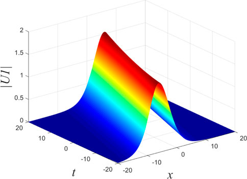
FIGURE 1. Single-soliton solution Eq. 39 with k = 0.12 + 0.26 * i.

4 Conclusion

The general coupled nonlinear integrable evolution equations and their N-soliton solutions on the time–space scale are formulated via employing the extensions of the GD formalism and standard DT on the time scale. By taking special values, we derive the Boussinesq equation on the time–space scale, and then, the classical Boussinesq equation and coupled semi-discrete Boussinesq equation are obtained by considering the continuous time scale $\mathbb{R}$ and discrete time scale $\mathbb{Z}$, respectively. Afterward, the exact solutions of the Boussinesq equation on the time–space scale are acquired via applying its DT, and the single-soliton solution of the classical Boussinesq equation is obtained as the special case. The extensions may supply more nonlinear integrable models and facilitate solving some practical problems unifying continuous and discrete cases. In the next, we will use the generalization of the GD formalism and DT to construct different integrable systems on time–space scales with other the higher-order δ differential operator so as to enrich the research of integrable systems on arbitrary time–space scales.

Data availability statement

The original contributions presented in the study are included in the article/Supplementary Material; further inquiries can be directed to the corresponding author.

Author contributions

XH, YZ, and HD contributed to the conception and design of the study. XH and YZ wrote sections of the manuscript. All authors contributed to manuscript revision, read, and approved the submitted version.

Funding

This work was supported by the National Natural Science Foundation of China (Grant Nos. 11975143, 12105161, and 61602188), the Natural Science Foundation of Shandong Province (Grant No. ZR2019QD018), the CAS Key Laboratory of Science and Technology on Operational Oceanography (Grant No. OOST2021-05), and the Scientific Research Foundation of Shandong University of Science and Technology for Recruited Talents (Grant Nos. 2017RCJJ068 and 2017RCJJ069).

Acknowledgments

The authors would like to express their thanks to the editors and the reviewers for their kind comments to improve our paper.

Conflict of interest

The authors declare that the research was conducted in the absence of any commercial or financial relationships that could be construed as a potential conflict of interest.

Publisher’s note

All claims expressed in this article are solely those of the authors and do not necessarily represent those of their affiliated organizations, or those of the publisher, the editors, and the reviewers. Any product that may be evaluated in this article, or claim that may be made by its manufacturer, is not guaranteed or endorsed by the publisher.

References

1. Ablowitz MJ, Segur H. Solitons and the inverse scattering transform. United States: SIAM (1981).

Google Scholar

2. Ablowitz MJ, Ladik J. Nonlinear differential-difference equations. J Math Phys (1975) 16:598–603. doi:10.1063/1.522558

CrossRef Full Text | Google Scholar

3. Dickey LA. Soliton equations and Hamiltonian systems. Singapore: World Scientific (1991).

Google Scholar

4. Silindir B, Prof A. Zero curvature and Gel’Fand-dikii formalisms. Ph.D. thesis. Turkey: Bilkent Universitesi (2004).

Google Scholar

5. Lebedev DR, Manin YI. Gel’fand–dikii Hamiltonian operator and the coadjoint representation of the volterra group. Funct Anal Appl (1979) 13:40–6. doi:10.1007/BF01078365

CrossRef Full Text | Google Scholar

6. Gel’Fand IM, Dikii LA. Asymptotic behaviour of the resolvent of sturm-liouville equations and the algebra of korteweg-de vries equations. Russ Math Surv (2007) 30:77–113. doi:10.1070/rm1975v030n05abeh001522

CrossRef Full Text | Google Scholar

7. GuRses M, Guseinov GS, Silindir B. Integrable equations on time scales. J Math Phys (2005) 46:113510. doi:10.1063/1.2116380

CrossRef Full Text | Google Scholar

8. Hilger S. Analysis on measure chains—A unified approach to continuous and discrete calculus. Results Math (1990) 18:18–56. doi:10.1007/bf03323153

CrossRef Full Text | Google Scholar

9. Bohner M, Peterson AC. Advances in dynamic equations on time scales. Germany: Springer Science & Business Media (2002).

Google Scholar

10. Bohner M, Peterson A. Dynamic equations on time scales: An introduction with applications. Germany: Springer Science and Business Media (2001).

Google Scholar

11. Hovhannisyan G, Bonecutter L, Mizer A. On burgers equation on a time-space scale. Adv Differ Equ (2015) 2015:289–19. doi:10.1186/s13662-015-0622-4

CrossRef Full Text | Google Scholar

12. Jator S. Block unification scheme for elliptic, telegraph, and sine-gordon partial differential equations. J Math Anal Appl (2015) 5:175–85. doi:10.4236/ajcm.2015.52014

CrossRef Full Text | Google Scholar

13. Hovhannisyan G, Ruff O. Darboux transformations on a space scale. J Math Anal Appl (2016) 434:1690–718. doi:10.1016/j.jmaa.2015.10.004

CrossRef Full Text | Google Scholar

14. Hovhannisyan G. Ablowitz-ladik hierarchy of integrable equations on a time-space scale. J Math Phys (2014) 55:102701. doi:10.1063/1.4896564

CrossRef Full Text | Google Scholar

15. Agarwal R, Bohner M, O’Regan D, Peterson A. Dynamic equations on time scales: A survey. J Comput Appl Math (2002) 141:1–26. doi:10.1016/s0377-0427(01)00432-0

CrossRef Full Text | Google Scholar

16. Ahlbrandt CD, Bohner M, Ridenhour J. Hamiltonian systems on time scales. J Math Anal Appl (2000) 250:561–78. doi:10.1006/jmaa.2000.6992

CrossRef Full Text | Google Scholar

17. Darboux G. Surune proposition relative aux equation lineaires. Paci Conserv Biol (1882) 94:145459.

Google Scholar

18. Gao XY. Variety of the cosmic plasmas: General variable-coefficient korteweg-de vries-burgers equation with experimental/observational support. Epl (2015) 110:15002. doi:10.1209/0295-5075/110/15002

CrossRef Full Text | Google Scholar

19. Zha QL, Li ZB. Darboux transformation and multi-solitons for complex mkdv equation. Chin Phys Lett (2008) 25:8–11. doi:10.1088/0256-307x/25/1/003

CrossRef Full Text | Google Scholar

20. Yesmakhanova K, Shaikhova G, Bekova G, Myrzakulov R. Darboux transformation and soliton solution for the (2+1)-dimensional complex modified korteweg-de vries equations. J Phys : Conf Ser (2017) 936:012045. doi:10.1088/1742-6596/936/1/012045

CrossRef Full Text | Google Scholar

21. Xu S, He J, Wang L. The Darboux transformation of the derivative nonlinear Schrödinger equation. J Phys A: Math Theor (2011) 44:305203. doi:10.1088/1751-8113/44/30/305203

CrossRef Full Text | Google Scholar

22. Fan EG. Darboux transformation and soliton-like solutions for the gerdjikov-ivanov equation. J Phys A: Math Gen (2000) 33:6925–33. doi:10.1088/0305-4470/33/39/308

CrossRef Full Text | Google Scholar

23. Guo BL, Ling LM, Liu QP. Nonlinear Schrödinger equation: Generalized darboux transformation and rogue wave solutions. Phys Rev E (2012) 85:026607. doi:10.1103/physreve.85.026607

PubMed Abstract | CrossRef Full Text | Google Scholar

24. Geng X. Lax pair and darboux transformation solutions of the modified boussinesq equation. Acta Math Appl Sin-e (1988) 11:324–8.

Google Scholar

25. Nimmo J. Darboux transformations for discrete systems. Chaos Solitons Fractals (2000) 11:115–20. doi:10.1016/s0960-0779(98)00275-6

CrossRef Full Text | Google Scholar

26. Dong HH, Huang XQ, Zhang Y, Liu MS, Fang Y. The darboux transformation and n-soliton solutions of gerdjikov–ivanov equation on a time–space scale. Axioms (2021) 10:294. doi:10.3390/axioms10040294

CrossRef Full Text | Google Scholar

27. Zakharov VE. On stochastization of one - dimensional chains of nonlinear oscillators. Soviet Phys (1973) 65:219–25. doi:10.1140/epjs/s11734-021-00420-6

CrossRef Full Text | Google Scholar

28. Clarkson PA, Kruskal M. New similarity reductions of the boussinesq equation. J Math Phys (1989) 30:2201–13. doi:10.1063/1.528613

CrossRef Full Text | Google Scholar

29. Ursell F. Trapping modes in the theory of surface waves. Math Proc Cambridge (1951) 47:347–58. doi:10.1017/S0305004100026700

CrossRef Full Text | Google Scholar

30. Bogdanov LV, Zakharov VE. The boussinesq equation revisited. Physica D: Nonlinear Phenomena (2002) 165:137–62. doi:10.1016/s0167-2789(02)00380-9

CrossRef Full Text | Google Scholar

31. Toda M. Studies of a non-linear lattice. Phys Rep (1975) 18:1–123. doi:10.1016/0370-1573(75)90018-6

CrossRef Full Text | Google Scholar

32. Khatun MA, Arefin MA, Uddin MH, Baleanu D, Akbar MA, Inc M. Explicit wave phenomena to the couple type fractional order nonlinear evolution equations. Results Phys (2021) 28:104597. doi:10.1016/j.rinp.2021.104597

CrossRef Full Text | Google Scholar

33. Zhang Y, Chang H, Li N. Explicit n-fold darboux transformation for the classical boussinesq system and multi-soliton solutions. Phys Lett A (2009) 373:454–7. doi:10.1016/j.physleta.2007.08.079

CrossRef Full Text | Google Scholar

34. Chen AH, Li XM. Darboux transformation and soliton solutions for boussinesq–burgers equation. Chaos Solitons Fractals (2006) 27:43–9. doi:10.1016/j.chaos.2004.09.116

CrossRef Full Text | Google Scholar

35. Lakshmikantham V, Sivasundaram S, Kaymakcalan B. Dynamic systems on measure chains. Germany: Springer Science & Business Media (2013).

Google Scholar