 Alexander Rothkopf
- Faculty of Science and Technology, University of Stavanger, Stavanger, Norway
The computation of dynamical properties of nuclear matter, ranging from parton distribution functions of nucleons and nuclei to transport properties in the quark-gluon plasma, constitutes a central goal of modern theoretical physics. This real-time physics often defies a perturbative treatment and the most successful strategy so far is to deploy lattice QCD simulations. These numerical computations are based on Monte-Carlo sampling and formulated in an artificial Euclidean time. Real-time physics is most conveniently formulated in terms of spectral functions, which are hidden in lattice QCD behind an ill-posed inverse problem. I will discuss state-of-the art methods in the extraction of spectral functions from lattice QCD simulations, based on Bayesian inference and emphasize the importance of prior domain knowledge, vital to regularizing the otherwise ill-posed extraction task. With Bayesian inference allowing us to make explicit the uncertainty in both observations and in our prior knowledge, a systematic estimation of the total uncertainties in the extracted spectral functions is nowadays possible. Two implementations of the Bayesian Reconstruction (BR) method for spectral function extraction, one for MAP point estimates and one based on an open access Monte-Carlo sampler are provided. I will briefly touch on the use of machine learning for spectral function reconstruction and discuss some new insight it has brought to the Bayesian community.
1 Introduction
1.1 The physics challenge
After a successful decade of studying the static properties of the strong interactions, such as their phase diagram (for reviews see e.g. [1, 2]) and equation of state (for recent studies see e.g., [3–5]) through relativistic heavy-ion collisions (for an overview see e.g., [6]) and more recently through the multi-messenger observations of colliding neutron stars (for a review see e.g. [7]), high energy nuclear physics sets out to make decisive progress in the understanding of real-time dynamics of quarks and gluons in the coming years.
The past heavy-ion collision campaigns at collider facilities such as RHIC at Brookhaven National Laboratory (BNL) and the LHC at the European Center for Nuclear Physics (CERN) provided conclusive evidence for the existence of a distinct high-temperature state of nuclear matter, the quark-gluon-plasma (for a review see e.g., [8]). At the same time, theory, by use of high-performance computing, predicted the thermodynamic properties, such as the equation of state [9–13] of hot nuclear matter from first principles. When data and theory were put to the test in the form of phenomenological models based on relativistic hydrodynamics, excellent agreement was observed (for a review see e.g., [14]).
Similarly past e−+p collider experiments at HERA (DESY) revealed (for a review see [15]) that the properties of nucleons can only be understood when in addition to the three valence quarks of the eponymous quark-model also the virtual excitations of quarks and gluons are taken into account. In particular the emergent phenomenon of asymptotic freedom manifests itself clearly in their data, as the coupling between quarks and gluons becomes weaker with increasing momentum exchange in a collision (for the current state-of-the art see e.g., [16]). Simulations of the strong interactions are by now able to map this intricate behavior of the strong coupling over a wide range of experimentally relevant scales, again leading to excellent agreement between theory and experiment (for a community overview see Chapter 9 of [17]).
Going beyond the static or thermodynamic properties of nuclear matter proves to be challenging for both theory and experiment. In heavy-ion collisions most observed particles in the final state at best carry a memory on the whole time-evolution of the collision. This requires phenomenology to disentangle the physics of the QGP from other effects e.g., those arising in the early partonic stages or the hadronic aftermath of the collision. It turns out that in order to construct accurate multi-stage models of the collision dynamics (see e.g., [18–20]), a variety of first-principles insight is needed. The dynamics of the bulk of the light quarks and gluons which make up the QGP produced in the collision is conveniently characterized by transport coefficients. Of central interest are the viscosities of deconfined quarks and gluons and their electric charge conductivity. The physics of hard probes, such as fast jets (see e.g., [21]) or slow heavy quark bound states (see e.g., [22]), which traverse the bulk nearly as test particles on the other hand requires insight into different types of dynamical quantities. In this context first principles knowledge of the complex in-medium potential between a heavy quark and antiquark, the heavy quark diffusion constant or the so-called jet quenching parameter
Going beyond merely establishing asymptotic freedom and instead revealing the full 6-dimensional phase space (i.e., spatial and momentum distribution) of partons inside nucleons and nuclei is the aim of an ambitious collider project just green-lit in the United States. The upcoming electron-ion collider [23] will be able to explore the quark and gluon content of nucleons in kinematic regimes previously inaccessible and opens up the first opportunity to carry out precision tomography of nuclei using well-controlled point-particle projectiles. Simulations have already revealed that the virtual particle content of nucleons is vital for the overall angular momentum budget of the proton (see e.g., [24, 25]). A computation of the full generalized transverse momentum distribution [26] however has not been achieved yet. This quantity describes partons in terms of their longitudinal momentum fraction x, the impact parameter of the collision bT and the transverse momentum of the parton kT. Integrating out different parts of the transverse kinematics leads to simpler object, such as transverse momentum distributions (TMDs, integrated over bT) or generalized parton distributions (GPDs, integrated over kT). Integrating all transverse dependence leads eventually to the conventional parton distribution functions (PDFs), which depend only on the longitudinal Bjorken x variable. A vigorous research community has made significant conceptual and technical progress over the past years, moving towards the first-principles determination of PDFs and more recently GPDs and TMDs from lattice QCD (for a community overview see [27]). Major advances in the past years include the development of the quasi PDF [28] and pseudo PDF [29] formalism, which offer complementary access to PDFs besides their well-known relation to the hadronic tensor [30]. With the arrival of the first exascale supercomputer in 2022, major improvements in the precision and accuracy of parton dynamics from lattice QCD are on the horizon.
1.2 Lattice QCD
In order to support experiment and phenomenology, theory must provide model independent, i.e., first-principles insight into the dynamics of quarks and gluons in nuclei and within the QGP. This requires the use of quantum chromo dynamics (QCD), the renormalizable quantum field theory underlying the strong interactions. Renormalizability refers to the fact that one only needs to provide a limited number of experimental measurements to calibrate each of its input parameters (strong coupling constant and quark masses) before being able to make predictions at any scale. In order to utilize this vast predictive power of QCD however we must be able to evaluate correlation functions of observables from their defining equations in terms of Feynman’s path integral
where
Computing the dynamical properties of quarks and gluons both inside nucleons as well as in the experimentally accessible QGP requires us to evaluate the above path integral in the presence of strong fluctuations, which invalidate commonly used weak-coupling expansions of the path integral weight. Instead a non-perturbative evaluation of observables is called for. While progress has been made in non-perturbative analytic approaches to QCD, such as the functional renormalization group [32, 33] or Dyson-Schwinger equations [34, 35], I focus here on the most prominent numerical approach: lattice QCD (for textbooks see e.g., [36, 37]).
In lattice QCD four-dimensional spacetime is discretized on a hypercube with N4 grid points n, separated by a lattice spacing a. In order to maintain the central defining property of QCD, the invariance of observables under local SU(3) rotations of quark and gluon degrees of freedom, in such a discrete setting, one introduces gauge link variables
It is the next and final step in the formulation of lattice QCD, which is crucial to understand the challenge we face in extracting dynamical properties from its simulations. The path integral of QCD, while already formulated in a discrete fashion, still contains the canonical complex Feynman weight
The action
Besides allowing us to incorporate the concept of temperature in a straight forward manner, this Euclidean path integral is now amenable to standard methods of stochastic integration, since the Euclidean Feynman weight is real and bounded from below. Using established Markov-Chain Monte Carlo techniques one generates ensembles of gauge field configurations distributed according to
here the error decreases with the number of generated configurations independent of the dimensionality of the underlying integral.
To avoid misunderstandings, let me emphasize that results obtained from lattice QCD at finite lattice spacing may not be directly compared to physical measurements. A valid comparison requires that the so-called continuum limit is taken a → 0, while remaining close to the thermodynamic limit V → ∞. Different lattice discretizations may yield deviating results, as long as this limit has not been adequately performed. For precision lattice QCD computations a community quality control has been established through the FLAG working group [17] to catalog different simulation results including information on the limits taken.
2 The inverse problem
The technical challenge we face is now laid bare: in order to make progress in the study of the dynamics of the strong interactions we need to evaluate Minkowski time correlation functions in QCD, related to parton distribution functions in nucleons or the dynamical properties of partons in the QGP. The lattice QCD simulations we are able to carry out however are restricted to imaginary time. Reverting back to the real-time domain as it turns out presents an ill-posed inverse problem.
The key to attacking this challenge is provided by the spectral representation of correlation functions [40]. It tells us that different incarnations of relevant correlation functions (e.g. the retarded or Euclidean correlators) share common information content in the form of a so-called spectral function [41]. The Källén–Lehmann representation reveals that the retarded correlator of fields in momentum space may be written as
while the same correlator in Euclidean time is given as
where the sign in the denominator differs between bosonic (−) and fermionic (+) correlators. Both real-time and Euclidean correlator therefore can be expressed by the same spectral function, integrated over different analytically known kernel functions.
As we do have access to the Euclidean correlator, extracting the spectral function from it in principle gives us direct access to its Minkowski counterpart. It is important to note that often phenomenologically relevant physics is encoded directly and intuitively in the structures of the spectral function, making an evaluation of the real-time correlator superfluous. Transport coefficients e.g., can be read off from the low frequency behavior of the zero-momentum spectral function of an appropriate correlation function [42].
For the extraction of parton distribution functions similar challenges ensue. PDFs can be computed from a quantity christened the hadronic tensor WM(t) [30], a four-point correlation function of quark fields in Minkowski time. The Euclidean hadronic tensor on the lattice is related to its real-time counterpart via a Laplace transform
that needs to be inverted. Recently the pseudo PDF approach [29] has shown how a less numerically costly three-point correlation function
where the Ioffe-time matrix elements
All the above examples of inverse problems share that they are in fact ill-posed. The concept of well- and conversely ill-posedness has been studied in detail and was first formalized by Hadamard [43]. Three conditions characterize a well posed problem: its solution exists, the solution is unique and the solution changes continuously with given initial conditions (which in our case refers to the supplied input data for the reconstruction task).
In the context of spectral function reconstruction, the latter two criteria present central challenges. Not only is the Euclidean correlator from the lattice Di known only at Nτ discrete points τi, but in addition, as it arises from Monte-Carlo simulations, it also carries a finite error ΔD/D ≠ 0. This entails that in practice an infinite number of spectral functions exist, which all reproduce the input data within their statistical uncertainties.
Even in the case that one could simulate a continuous correlator, the stability of the inversion remains an issue. The reason is that as one simulates on limited domains, be it limited in Euclidean time due to a finite temperature (transport coefficients) or limited in Ioffe time (PDFs) the inversion exhibits strong sensitivity on uncertainties in the input data. The presence of exponentially small eigenvalues in the kernel K renders the inversion task in general ill-conditioned.
To be more concrete, let us write down the discretized spectral representation in terms of a spectral function ρl discretized at frequencies μl along Nμ equidistant frequency bins of with Δμl and the discretized kernel matrix Kil
The task at hand is to solve the inverse problem of determining the parameters ρl from the sparse and noisy Di’s. The ill-posedness of this inverse problem is manifest in Eq. 8 in two aspects:
State-of-the-art lattice QCD simulations provide only around
In addition many of the kernel functions we have to deal with are of exponential form. This entails a strong loss of information between the spectral function and the Euclidean correlator. In other words, large changes in the spectral function translate into minute changes in the Euclidean correlator. Indeed, each of the tiny eigenvalues of the kernel is associated with a mode along frequencies, which can be added to the spectral function without significantly changing the correlator. Reference [44] has recently investigated this fact in detail analytically for the bosonic finite temperature kernel relevant in transport coefficient computations.
Even the at first sight benign cos kernel matrix arising in the pseudo PDF approach turns out to feature exponentially diminishing eigenvalues [45] as the lattice simulation cannot access the full Brillouin zone in ν. I.e., the matrix Kil is in general ill-conditioned, making its inversion unstable even if no noise is present. In the presence of noise the exponentially small eigenvalues lead to a strong enhancement of even minute uncertainties in the correlation functions rendering the inversion meaningless without further regularization.
We will see in the next section how Bayesian inference and in particular the inclusion of prior knowledge can be used to mitigate the ill-posed (and ill-conditioned) nature of the inversion task and give meaning to the spectral function reconstruction necessary for extracting real-time dynamics from lattice QCD.
3 Bayesian inference of spectral functions
The use of Bayesian inference to extract spectral functions from lattice QCD simulations was pioneered by a team of researchers from Japan in two seminal papers [46, 47]. Inspired by prior work in condensed matter physics [48] and image reconstruction [49], the team successfully transferred the approach to the extraction of QCD real-time information. The work sparked a wealth of subsequent studies, which have applied and further developed Bayesian techniques to the extraction of real-time information from lattice QCD in various contexts, zero temperature hadron spectra and excited states [50–52], parton-distribution functions [45, 53], in-medium hadrons [54–67], sum rules [68, 69], transport coefficients [42, 70–76, 76], the complex in-medium heavy quark potential [77–80] and parton spectral properties [81–83].
The following discussion focuses on the Bayesian extraction of spectral functions that does not rely on a fixed parametrization of the functional form of ρ. If strong prior information exists, e.g. if vacuum hadronic spectral functions consist of well separated delta peaks, direct Bayesian parameter fitting methods are applicable [84] and may be advantageous. Similarly, some studies of in-medium spectra and transport phenomena deploy explicit parametrization of the spectral function derived from model input, whose parameters can be fitted in a Bayesian fashion (see Ref. [85] for a recent example). Our goal here is to extract spectral features for systems in which no such apriori parametrization is known.
3.1 Bayesian inference
Bayesian inference is a sub-field of statistical data analysis (for an excellent introduction see e.g., [86, 87]), which focuses on the estimation of unobserved quantities, based on incomplete and uncertain observed data (see Figure 1). The term unobserved is used to refer to the unknown parameters governing the process, which generates the observed data or to as of yet unobserved future data. In the context of the inverse problem in lattice QCD, the Euclidean correlation functions produced by a Monte-Carlo simulation take on the role of the observed data while the unobserved parameters are the values of the discretized spectral function ρl. Future observations can be understood as further realizations of the Euclidean correlator along the Markov-Chain of the simulation.
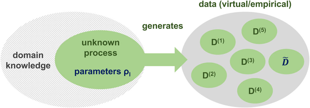
FIGURE 1. Statistical inference attempts to estimate from observed data D(k) the unknown process parameters ρl and as of yet unobserved data
What makes Bayesian inference particularly well suited to attack the inverse problem is that it offers an explicit and well controlled strategy to incorporate information (I) beyond the measured data (D) into the reconstruction of spectral functions (ρ). It does so by using a more flexible concept of probability, which does not necessarily rely on the outcome of a large number of repeatable trials but instead assigns a general degree of uncertainty.
To be more concrete, Bayesian inference asks us to acknowledge that any model of a physical process is constructed within the context of its specific domain, in our case strong interaction physics. I.e., the structure of the model and its parameters are chosen according to prior information obtained within its domain. Bayesian inference then requires us to explicitly assign degrees of uncertainty to all these choices and propagate this uncertainty into a generalized probability distribution called the posterior P[ρ|D, I]. Intuitively it describes how probable it is that a test function ρ is the correct spectral function, given simulated data D and prior knowledge I.1
The starting point of any inference task is the joint probability distribution P[ρ, D, I]. As it refers to the parameters ρ, data D and prior information I it combines information about the specific process generating the data as well as the domain it is embedded in. After applying the rules of conditional probability one obtains the work-horse of Bayesian inference, the eponymous Bayes theorem
It tells us how the posterior P[ρ|D, I] can be efficiently computed. The likelihood denotes the probability for the data D to be generated from QCD given a fixed spectral function ρ. The prior probability quantifies how compatible ρ is compared to our domain knowledge. Historically the ρ independent normalization has been called the evidence. Let us construct the different ingredients to Bayes theorem in the following.
What is the likelihood in the case of spectral function reconstruction? In Monte-Carlo simulations one usually computes sub-averages of correlation functions on each of the Nconf generated gauge field configurations. For many commonly studied correlation functions, thanks to the central limit theorem, such data already approximate a normal distribution to a good degree. It is prudent to check the approach to Gaussianity for individual correlation functions, as it has been revealed in Refs. [88, 89] that some actually exhibit a log-normal distribution which converges only very slowly.
In case that the input data is approximately normal distributed, the corresponding likelihood probability P[D|ρ, I] ∝ exp[−L], written in terms of the likelihood function L, too is a multidimensional Gaussian
where Di denotes the mean of the simulated data at the ith Euclidean time step and
where the individual measurements enter as D(k). Note that in order to obtain an accurate estimate of Cij, the number of samples Nconf must be significantly larger than the number of data along imaginary time. In particular Cij develops exact zero eigenvalues if the number of configurations is less than that of the datapoints.
In lattice QCD simulations, which are based on Monte-Carlo sampling, correlators computed on subsequent lattices are often not statistically independent. At the same time Eq. 11 assumes that all samples are uncorrelated. Several strategies are deployed in the literature to address this discrepancy. One common approach is to rely on resampling methods, such as the (blocked) Jackknife (for an introduction see Ref. [90]) or similar bootstrap methods in order to estimate the true covariance matrix. Alternatively one may compute the exponential autocorrelation time
A speedup in the computation of the likelihood can be achieved in practice if, following Ref. [46], one computes the eigenvalues σi and eigenvectors of C and changes both the kernel and the input data into the coordinate system where StCS = diag[σi] becomes diagonal. Then the two sums in Eq. 10 collapse onto a single one
Since the likelihood is a central ingredient in the posterior, all Bayesian reconstruction methods ensure that the reconstructed spectral function, when inserted into the spectral representation will reproduce the input data within their uncertainty. I.e., they will always produce a valid statistical hypothesis for the simulation data. This crucial property distinguishes the Bayesian approach from competing non-Bayesian methods, such as the Backus-Gilbert method and the Padé reconstruction (see examples in e.g., [91, 92]), in which the reconstructed spectral function does not necessarily reproduce the input data.
In case that we do not possess any prior information we have P[ρ|I] = 1 and Bayes theorem only contains the likelihood. Since the functional L is highly degenerate in terms of ρl’s, the question of what is the most probable spectral function, i.e., the maximum likelihood estimate of ρ, does not make sense at this point. Only by supplying meaningful prior information can we regularize and thus give meaning to the inverse problem.
3.2 Bayesian spectral function reconstruction
Different Bayesian strategies to attack the ill-posed spectral function inverse problem differ by the type of domain information they incorporate in the prior probability P[ρ|I] ∝ exp[S], where S is called the regulator functional. Once the prior probability is constructed, the spectral reconstruction consists of evaluating the posterior probability P[ρ|D, I], which informs us of the distribution of the values of ρl in each frequency bin μl.
The versatility of the Bayesian approach actually allows us to reinterpret several classic regularization prescriptions in the language of Bayes theorem, providing a unifying language to seemingly different strategies.
When surveying approaches to inverse problems in other fields, Tikhonov regularization [93] is by far the most popular regularization prescription. It amounts to choosing an independent Gaussian prior probability for each parameter
Each normal distribution is characterized by its maximum (mean) denoted here by ml and width (uncertainty)
Another regularization deployed in the field of image reconstruction is the so-called total variation approach [94]. Here the difference between neighboring parameters ρl and ρl+1, i.e., Δρl, is modelled [95] as a Laplace distribution
Since Δρl is related to the first derivative of the spectral function this regulator incorporates knowledge about rapid changes, such as kinks, in spectral features. Choosing αl and ml appropriately one may e.g., prevent the occurrence of kink features in the reconstructed spectral function, if it is known that the underlying true QCD spectral function is smooth.
In Ref. [96] I proposed a regulator related to the derivative of ρ, with a different physical meaning
Often spectral reconstructions, which are based on a relatively small number of input data, suffer from ringing artifacts, similar to the Gibbs ringing arising in the inverse problem of the Fourier series. These artifacts lead to a reconstructed spectral function with a similar area as the true spectral function but with a much larger arc length due to the presence of unphysical wiggles. Since such ringing is not present in the true QCD spectral function we may apriori suppress it by penalizing arc length
If our prior domain knowledge contains information about the smoothness and the absence of ringing then it is of course possible to combine different regulators by multiplying the prior probabilities. The reconstruction of the first picture of a black hole e.g., combined the Tikhonov and total variation regularization [97]. In the presence of multiple regulators, the hyperparameters α and m of each of these distributions need to be assigned an (independent) uncertainty distribution.
One may ask, whether a proliferation of such parameters spoils the benefit of the Bayesian approach? The answer is that in practice one can estimate the probable ranges of these parameters by use of mock data. One carries out the spectral function reconstruction, i.e., the estimation of the posterior probability P[ρ|D, I], using data, which has been constructed from known spectral functions with realistic features and which has been distorted with noise similar to those occurring in Monte-Carlo simulations (see e.g., [67]). One may then observe from such test data sets, what the most probable values of the hyperparameters are and in what interval they vary, depending on different spectral features present in the input data.
The three priors discussed so far are not commonly used as stand-alone regulators in the reconstruction of hadron spectral functions from lattice QCD in practice. The reason is that neither of them can exploit a central prior information available in the lattice context, which is the positivity [36] of the most relevant hadronic spectral functions. I.e., in most of the relevant reconstruction tasks from lattice QCD, the problem can be formulated in terms of a positive definite spectral function, which significantly limits the function space of potential solutions. Methods that are unable to exploit this prior information, such as the Backus-Gilbert method have therefore been shown to perform poorly relative to the Bayesian approaches, when it comes to the reconstruction of well-defined spectral features (see e.g., [53]).
In the following let us focus on two prominent Bayesian methods, which have been deployed in the reconstruction of positive spectral functions from lattice QCD, the Maximum Entropy Method (MEM) and the Bayesian Reconstruction (BR) method.
The MEM [47–49, 98] has originally been constructed to attack image reconstruction problems in astronomy. It therefore focuses on two-dimensional input data and deploys the Shannon-Jaynes entropy SSJ as regulator:
Its regulator is based on four axioms [49], which specify the prior information the method exploits. They are subset independence, which states that prior information on ρl’s at different discrete frequency bins l can be combined in a linear fashion within SSJ. The second axiom enforces that SSJ has its maximum at the default model, which establishes the meaning of ml as the apriori most probable value of ρl in the absence of data. These two axioms are not specific to the MEM and find use in different Bayesian methods. It is the third and fourth axiom that distinguish the MEM from other approaches: coordinate invariance requires that ρ itself should transform as a dimensionless probability distribution. To be more concrete, as MEM was constructed with image reconstruction in mind, this axiom requires that the reconstructed image (in our case the spectral function) should be invariant under a common coordinate transformation of the two-dimensional input data and the prior. The last axiom is system independence and requires that in a two-dimensional reconstructed image no additional correlations between the two dimensions of the image are introduced, beyond those that are already contained in the data (for more details see Ref. [99]).
From the appearance of the logarithm in SSJ it is clear that the MEM can exploit the positivity of the spectral function. Due to the fact that the logarithm is multiplied by ρ, SSJ is actually able to accommodate exact zero values of a spectral function. Since the reconstruction task in lattice QCD is one-dimensional, it is not obvious how to directly translate system independence. An intuitive way of interpreting this axiom using e.g. the kangaroos example of Ref. [48] is that the MEM shall not introduce correlations among ρl’s where the data does not require it. This is a quite restrictive property, as it is exactly prior information, which should help us to limit the potential solutions space by providing as much information about the structure of ρ as possible. Similarly, the assumption that ρ must transform as a probability distribution, while appropriate for a distribution of dimensionless pixel values in an image, does not necessarily apply to spectral functions. These are in general dimensionful quantities and may even contain UV divergences when evaluated naively.
To overcome these conceptual difficulties the BR method was developed in Ref. [100] with the one-dimensional reconstruction problem of lattice QCD real-time dynamics in mind. The BR method features a regulator SBR related to the Gamma distribution
which looks similar to the Shannon-Jaynes entropy but differs in crucial ways. Its construction shares the first two axioms of the MEM but replaces the third and fourth axiom with the following: scale invariance enforces that the posterior may not depend on the units of the spectral function, leading to only ratios between ρl and the default model ml, which by definition must share the same units. The use of ratios also requires that neither ρ nor m vanishes. SBR differs therefore from the Shannon-Jaynes regulator where the integrand of SSJ is dimensionful. The units of Δμ enter as multiplicative scale and can be absorbed into a redefinition of α (and which will be marginalized over as described in Section 3.3). Furthermore, one introduces a smoothness axiom, which requires the spectral function to be twice differentiable. While it may appear that the latter axiom is at odds with the potential presence of delta-function like structures in spectral functions, it ensures that one smoothly approximates such well defined peaks as the input data improves.
Let us compare the regulators of the Tikhonov approach, the MEM and the BR method in Figure 2, which plots the negative of the integrand for the choice of m = 1. The top panel shows a linear plot, the bottom panel a double logarithmic plot. By construction, all feature an extremum at ρ = m.
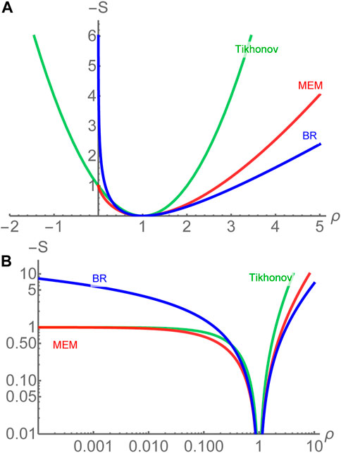
FIGURE 2. Comparison of the regulators of the Tikhonov approach (green), the MEM (red) and the BR method (blue) in linear scale (A) and double logarithmic scale (B) for the choice of m = 1. The Shannon-Jaynes regulator accommodates ρ = 0 but appears flat for spectral functions with values close to zero. The BR prior shows the weakest curvature for ρ > m among all regulators.
The functional form of the BR regulator turns out to be the one with the weakest curvature among all three for ρ > m, while it still manages to regularize the inverse problem. Note that the weaker the regulator, the more efficiently it allows information in the data to manifest itself (it is actually the weakest on the market). At the same time a weaker regulator is less potent in suppressing artifacts, such as ringing, which may affect spectral function reconstruction based on very small number of datapoints.2
Note that the BR regulator requires ρ to be positive definite, whereas the MEM accommodates spectral functions and default models that vanish identically over a range of frequencies. In hadronic spectra, e.g., it is known that the spectral function can vanish in regions below threshold. While in the MEM this fact can be incorporated naturally, in the BR method a small but finite value must be supplied in the default model everywhere. In practice this is most often not a problem, since it is below threshold where the non-perturbative bound state structures lie that one wishes to reconstruct. Hence reliable prior information is in general not available and one chooses an uninformative finite, i.e. constant default model there.
Having focused primarily on positive spectral functions so far, let us briefly discuss some of the Bayesian approaches used in the literature to study non-positive spectral functions. This task may arise in the context of hadron spectral functions if correlators with different source and sink operators are investigated (see e.g., Discussion in [101]) or if the underlying lattice simulation deploys a Szymanzik improved action (see e.g., [102]). The quasiparticle spectral functions of quarks and gluons are known to exhibit positivity violation, their study from lattice QCD therefore apriori requires methods that can accommodate spectral functions with both positive and negative values. We already saw that the Tikhonov approach with Gaussian prior does not place restrictions on the values of the spectral function and has therefore been deployed in the study of gluon spectral functions in the past [81, 83]. After the development of the MEM, Hobson and Lasenby [103] extended the method by decomposing general spectral functions into a positive (semi-)definite and negative (semi-)definite part. To each of these a Shannon-Jaynes prior is assigned. The third approach on the market is an extension of the BR method [104], which relaxes the scale invariance axiom and proposes a regulator that is symmetric around ρ = m. This method has been deployed in the study of gluon spectral functions [82] and in the extraction of parton distribution functions [45].
An alternative that is independent of the underlying Bayesian approach (see e.g., [105]) is to add to the input data that of a known, large and positive mock-spectral function, which will compensate for any negative values in the original spectral function. After using a Bayesian method for the reconstruction of positive ρs from the modified data, one can subtract from the result the known mock spectral function. In practice this strategy is found to require very high quality input data to succeed.
The challenge one faces in the reconstruction of non-positive spectral functions is that the inversion task becomes significantly more ill-posed in the sense of non-uniqueness. Positivity is a powerful constraint that limits admissible functions that are able to reproduce the input data. In its absence, many of the functions associated with small and even vanishing singular values of the kernel K can contaminate the reconstruction. Often these spurious functions exhibit oscillatory behavior which interferes with the identification of genuine physical peak structures encoded in the data (see also discussion in [91]).
Having surveyed different regulator choices, we are ready to carry out the Bayesian spectral reconstruction. I.e. after choosing according to one’s domain knowledge a prior distribution P[ρ|I(m, α)] and assigning appropriate uncertainty intervals to their hyperparameters P[α] and P[m] via mock-data studies, we can proceed to evaluate the posterior distribution P[ρ|D, I]. If we can access this highly dimensional object through a Monte-Carlo simulation (see e.g., Section 4.3) it provides us not only with the information of what the most probable spectral function is, given our simulation data, but also contains the complete uncertainty budget, including both statistical (data related) and systematic errors (hyperparameter related). The maximum of the prior defines the most probable value for each ρl and its spread allows a robust uncertainty quantification beyond a simple Gaussian approximation (i.e., standard deviation) as it may contain tails that lead to a deviation of the mean from the most probable value.
3.3 Uncertainty quantification for point estimates
While access to the posterior allows for a comprehensive uncertainty analysis, a full evaluation of P[ρ|D, I] historically remained computationally prohibitive. Thus the community focused predominantly3 on determining a point estimate of the most probable spectral function from the posterior P[ρ|D, I], also called MAP, the maximum aposteriori estimate
where in practice often the logarithm of the posterior is used in the actual optimization
While estimating the MAP, i.e., carrying out a numerical optimization, is much simpler than sampling the full posterior, only a fraction of the information contained in P[ρ|D, I] is made accessible. In particular most information related to uncertainty remains unknown and thus needs to be approximated separately.
The above optimization problem in general can be very demanding as the posterior may contain local extrema in addition to the global one that defines ρMAP (see sketch in Figure 3). At least in the case of the Tikhonov, MEM and BR method it is possible to prove that if an extremum for Eq. 17 exists it must be unique. The reason is that all three regulators are convex. The proof of this statement does not rely on a specific parametrization of the spectral function and therefore promises that standard (quasi)Newton methods, such as Levenberg-Marquardt or LBFGS (see e.g., Ref. [110]) can be used to locate this unique global extremum in the Nμ dimensional search space.
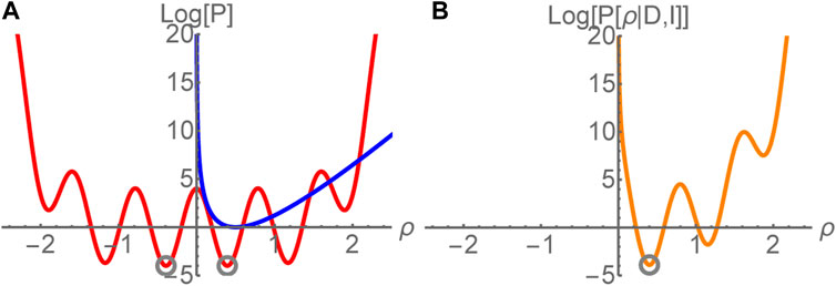
FIGURE 3. Sketch of how the confluence of (A) likelihood (red) and (a convex) prior (blue) in the posterior [orange, (B)] leads to a regularization of the inverse problem. Instead of multiple degenerate minima in the likelihood (gray circles) only a single unique one remains in the posterior.
Also from an information point of view it is fathomable that at this point a unique solution to the former ill-posed inverse problem can be found. We need to estimate the most probable values of Nμ parameters ρl and have now provided Nτ simulation data Di, as well as Nμ pieces of information in the form of the ml’s and αl’s each. I.e., the number of knowns 2Nμ+Nτ > Nμ is larger than the number of unknowns, making a unique determination possible. The proof presented in Ref. [47] formalizes this intuitive statement.
In practice it turns out that the finite intercept of the Shannon-Jaynes entropy for ρ = 0 can lead to slow convergence if spectral functions with wide ranges of values close to zero are reconstructed. In lattice QCD this occurs regularly when e.g. hadronic spectral functions contain sharp and well separated peak structures. SSJ for very small values (see Figure 2) is effectively flat and thus unable to efficiently guide the optimizer toward the unique minimum and convergence slows down.
It is therefore that one finds in the literature that the extremum Eq. 17 in the MEM is accepted for tolerances around Δ ≈ 10−7, which is much larger than zero in machine (double-)precision. Such a large tolerance does not guarantee bitwise identical results when starting the optimization from different initial conditions. Note that the definition of Δ varies in the literature and we here define it via the relative step size in the minimization of the optimization functional
The BR prior on the other hand does not exhibit a finite intercept at ρ = 0 and therefore avoids this slow convergence problem. It has been found to be capable of locating the unique extremum ρMAP in real-world settings down to machine precision, which guarantees that the reconstruction result is independent of the starting point of the optimizer.
Bayesian inference, through the dependencies of the posterior P[ρ|D, I], forces us to acknowledge that the result of the reconstruction is affected by two sources of uncertainty: statistical uncertainty in the data and systematic uncertainty associated with the choice and parameters of the prior probability.
Before continuing to the technical details of how to estimate uncertainty, let us focus on the role of prior information first. It enters both through the selection of a prior probability and the choice of the distributions P[m] and P[α]. It is important to recognize that already from an information theory viewpoint, one needs to supply prior information if the goal is to give meaning to an ill-posed inverse problem: originally we started out to estimate Nμ ≫ Nτ parameters ρl from Nτ noisy input data Di.
I.e., in order to select among the infinitely many degenerate parameter sets ρl a single one as the most probable, we need information beyond the likelihood. Conversely any method that offers a unique answer to the inverse problem utilizes some form of prior information, whether it acknowledges it or not. Bayesian inference, by making the role of prior knowledge explicit in Bayes theorem, allows us to straight forwardly explore the dependence of the result on our choices related to domain information. It is therefore ideally suited to assess the influence of prior knowledge on reconstructed spectral functions. This distinguishes it from other approaches, such as the Backus Gilbert method, where a similarly clear distinction of likelihood and prior is absent. The Tikhonov method is another example. Originally formulated with a vanishing default model, one can find statements in the literature that it is default model independent. Reformulated in the Bayesian language, we however understand that its original formulation just referred to one specific choice of model, which made the presence of prior knowledge hard to spot.
The presence of the prior as regulator also entails that among the structures in a reconstructed spectral function only some are constrained by the simulation data and others are solely constrained by prior information. It is only in the Bayesian continuum limit, which refers to taking simultaneously the error on the input data to zero while increasing the number of available datapoints toward infinity, that the whole of the spectral function is fixed by input data alone. Our choice of regulator determines how efficiently we converge to this limit and which type of artifacts (e.g., ringing or over-damping) one will encounter on the way. One important element of uncertainty analysis in Bayesian spectral reconstruction therefore amounts to exploring how reconstructed spectra improve as the data improves.4 This is a well-established practice in the community.
When reconstructing the spectral function according to a given set of Monte–Carlo estimates
In the case of point estimates, one usually decides apriori on a regulator and fixes to a certain value of the default model m and of the hyperparameter α, before carrying out the reconstruction. The freedom in all these choices enters the systematic uncertainty budget.
Often the user has access to a reliable default model m(ω) only along a limited range of frequencies μ. In lattice QCD such information is often obtained from perturbative computations describing the large frequency and momentum behavior of the spectral function (see e.g. [111–114]). When considering continuum perturbative results as default model one must account for the finite lattice spacing by introducing a cutoff by hand. In addition the different (re-)normalization schemes in perturbation theory and on the lattice often require an appropriate rescaling. Subsequently, perturbative default models can reproduce input datapoints dominated by the spectrum at large frequencies (e.g., small Euclidean times). One additional practical challenge lies in the functional form of spectral functions obtained from (lattice) perturbation theory, since they may exhibit kink structures. If supplied as default model, as is, such structures may induce ringing artifacts in the reconstructed result. In practice one therefore smooths out kink structures when constructing m(ω).
In the low frequency part of the spectrum, where non-perturbative physics dominates, we often do not possess relevant information about the functional form of ρ. It is then customary to extend the default model into the non-perturbative regime using simple and smooth functional forms that join up in the perturbative regime.
In practice the user repeats the reconstruction using different choices for the unknown parts of m, e.g., different polynomial dependencies on the frequency and subsequently uses the variation in the end result as indicator of the systematic uncertainty. It is important to note that if there exist different regulators that encode compatible and complementary prior information that one should also consider repeating the reconstruction based on different choices of P[ρ|I] itself.
Since we have access to the likelihood and prior, we may ask whether a combined estimation of the statistical and systematic uncertainty can be carried out even in the case of a point estimate. Since the reconstructed spectrum ρMAP denotes a minimum of the posterior, one may try to compute the curvature of the (log) posterior L−S around that minimum, which would indicate how steep or shallow that minimum actually is. This is the strategy laid out e.g., in Ref. [47]. In practice it relies on a saddle point approximation of the posterior and therefore can lead to an underestimation of the uncertainty. Many recent studies thus deploy a combination of the Jackknife and a manual variation of the default model.
Since the treatment of hyperparameters differs among the various Bayesian methods, let me discuss it here in more detail. Appropriate ranges for the values of m can often be estimated from mock data studies and since the functional dependence of the default model is varied as part of the uncertainty estimation discussed above, we focus here on the treatment of α. I.e., we will treat the values of m as fixed and consider the effect of P[α]. If alpha is taken to be small, a large uncertainty in the value m ensues, which leads to a weak regularization and therefore to large uncertainty in the posterior. If α is large it constrains the posterior to be close to the prior and limits the information that data can provide to the posterior.
Three popular strategies are found in the literature to treat α. Note that in the context of the MEM, a common value is assigned to all hyperparameters αl, i.e., the same uncertainty is assigned to the default model parameters ml at all frequencies, an ad hoc choice.
The simplest treatment of α, also referred to as the Morozov criterion or historic MEM is motivated by the goal to avoid over fitting of the input data. It argues that if we knew the correct spectral function and were to compute the corresponding likelihood function L, it would on average evaluate to
The second and third strategy are based directly on Bayes theorem. The Bayesian way of handling uncertainties in model parameters is to make their dependence explicit in the joint probability distribution P[ρ, D, I(m, α)]. Now that the distribution depends on more than three elements, application of conditional probabilities leads to
The modern MEM approach solves Eq. 18 for P[α|ρ, D, m]. It then integrates point estimates
Let me briefly clarify the often opaque notion of Jeffrey’s prior [115]. Given a probability distribution P[x|α, m] and a choice of parameter, e.g., α, Jeffrey’s prior refers to the unique distribution
Jeffrey’s prior for m is independent of m and thus refer to the unique translation invariant distribution on the real values (Haar-measure for addition). It therefore does not impart any information on the location of the peak of the normal distribution. Similarly PJ[σ] is a scale invariant distribution on the positive real values (Haar-measure for multiplication). Since the uncertainty parameter σ enters as a multiplicative scale in the normal distribution its Jeffrey’s prior also does not introduce any additional information. Both priors investigated here are improper distributions, i.e., they are well-defined only in products with proper probability distributions.
The third strategy to treat the parameters αl has been put forward in the context of the BR method. It sets out to overcome the two main limitations of the MEM approach: the need for saddle point approximations in the handling of α and the overly restrictive treatment of assigning a common uncertainty to all ml’s. The BR method succeeds in doing so, by using Bayes theorem to marginalize the parameters αl apriori, making the (highly conservative) assumption that no information about αl is known, i.e., P[αl] = 1. It benefits from the fact that in contrast to the Shannon-Jaynes prior, the BR-prior is analytically tractable and its normalization can be expressed in closed form.
We start from Eq. 18 and assume that the parameters α and m are independent, so that their distributions factorize. Marginalizing a parameter simply means integrating the posterior over the probability distribution of that parameter. Via application of conditional probabilities it is possible to arrive at the corresponding expression
where P[ρ|D, m] does not depend on α anymore and by definition of probabilities ∫dαP[α|ρ, D, m] = 1. The posterior P[ρ|D, m] now includes all effects arising from the uncertainty of α without referring to that variable anymore. Due to the form of the BR prior P[ρ|α, m], the integral over αl is well defined, even though we used the improper distribution P[α] = 1. One may wonder whether integrating over αl impacts the convexity of the prior. While not proven rigorously, in practice it turns out that the optimization of the marginalized posterior P[ρ|D, m] in the BR method does not suffer from local extrema.
A user of the BR method therefore only needs to provide a set of values for the default model ml to compute the most probable spectral function
By carrying out several reconstructions and varying the functional form of m within reasonable bounds, established by mock-data tests, the residual dependence on the default model can be quantified.
So far we have discussed the inherent uncertainties from the use of Bayesian inference and how to assess them. Another source of uncertainty in spectral reconstructions arises from specific implementation choices. Let me give an example based on the Maximum Entropy Method. In order to save computational cost, the MEM historically is combined with a singular value decomposition to limit the dimensionality of the solution space. The argument by Bryan [116] suggests that instead of having to locate the unique extremum of P[ρ|D, I] in the full Nμ dimensional search space of parameters ρl, it is sufficient to use a certain parametrization of ρ(μ) in terms of Nτ parameters, the number of input data points. The basis functions are obtained from a singular value decomposition (SVD) of the transpose of the kernel matrix Kt. Bryan’s argument only refers to the functional form of the Kernel K and the number of data points Nτ in specifying the parametrization of ρ(μ). If true in general, this would lead to an enormous reduction in computational complexity. However, I have put forward a counter example to Bryan’s argument (originally in [117]) including numerical evidence, which shows that in general the extremum of the prior is not part of Bryan’s reduced search space.
One manifestation of the artificial limitation of Bryan’s search space is a dependence of the MEM resolution on the position of a spectral feature along the frequency axis. As shown in Figure 3 of Ref. [118], if one reconstructs a single delta peak located at different positions μ0 with the MEM, one finds that the reconstructed spectral functions show a different width, depending on the value of μ0. This can be understood by inspecting the SVD basis functions, which are highly oscillatory close to μmin the smallest frequency chosen to discretize the μ range. At larger values of μ these functions however damp towards zero. I.e. if the relevant spectral feature is located in the μ range where the basis functions have structure, it is possible to reconstruct a sharp peak reasonable well, while if it is located at larger μ the resolution of the MEM decreases rapidly. The true Bayesian ρMAP, i.e. the global extremum of the MEM posterior, however does not exhibit such a resolution restriction, as one can see when changing the parametrization of the spectral function to a different basis, e.g., the Fourier basis consisting of cos and sin functions. In addition Ref. [57] in its Figure 28 showed that using a different parametrization of the spectral function, which restricts ρ to a space that is equivalent to the SVD subspace from a linear algebra point of view, one obtains a different result. This, too, emphasizes that the unique global extremum of the posterior is not accessible within these restricted search spaces. Note that one possible explanation for the occurrence of the extremum of P[ρ|D, I] outside of the SVD space lies the fact that in constrained optimization problems (here the constraint is positivity), the extremum can either be given by the stationarity condition of the optimization functional in the interior of the search space or it can lie on the boundary of the search space restricted by the constraint.
I.e., in addition to artifacts introduced into the reconstructed spectrum via a particular choice of prior distribution and handling of its hyperparameters (e.g., ringing or over-damping), one also must be aware of additional artifacts arising from choices in the implementation of each method.
The dependence of Bryan’s MEM on the limited search space was among the central reasons for the development of the BR method. The advantageous form of the BR prior, which does not suffer from slow convergence in finding ρMAP in practice, allows one to carry out the needed optimization in the full Nμ dimensional solution space to P[ρ|D, I] with reasonable computational cost. The proof from Ref. [47] which also applies to the convex BR prior, guarantees that in the full search space a single unique Bayesian solution can be located if it exists.
In Section 4 we will take a look at hands-on examples of using the BR method to extract spectral functions and estimating their reliability.
3.4 Two lattice QCD uncertainty challenges
Spectral function reconstruction studies from lattice QCD have encountered two major challenges in the past.
The first one is related to the number of available input data points, which, compared to simulations in e.g. condensed matter physics is relatively small, of the order O(10−100). Especially when analyzing datasets at the lower end of this range, the sparsity of the Di’s along Euclidean time τ often translates into ringing artifacts. Due to the restricted search space of Bryan’s MEM, this phenomenon may be hidden, while the global extremum of the MEM posterior
The second challenge affects predominantly spectral reconstructions at finite temperature, in particular their comparability at different temperatures. In lattice QCD, temperature is encoded in the length of the imaginary time axis. I.e., simulations at lower temperature have access to a larger τ regime, as those at higher temperature. Since the available Euclidean time range affects the resolution capabilities of any spectral reconstruction it is important to calibrate one’s results to a common baseline. I.e., one needs to establish how the accuracy of the reconstruction method changes as one increases temperature. Otherwise changes in the reconstructed spectral functions are attributed to physics, while they actually represent simply a degradation of the method’s resolution. The concept of the reconstructed correlator [55] is an important tool in this regard. Assume we have a correlator encoding a certain spectral function at temperature T1 with
By carrying out a reconstruction based on two correlators at different Euclidean extent Dlattice(τ|T1) and Dlattice(τ|T2) one will in general obtain two different spectral functions. Only when one compares the reconstruction based on Drec(τ, T2|T1) with that of Dlattice(τ|T2) is it possible to disentangle the genuine effects of a change in temperature from the one’s induced by the reduction in access to Euclidean time. This reconstruction strategy has been first deployed for relativistic correlators in Ref. [66]. A similar analysis in the context of non-relativistic spectral functions in Ref. [67] showed that the temperature effect of a negative mass shift for in-medium hadrons was only observable, if the changes in resolution of the reconstruction had been taken into account.
4 Hands-on spectral reconstruction with the BR method
This publication is accompanied by two open-source codes. The first [119], written in the C/C++ language, implements the BR method (and the MEM) in its traditional form to compute MAP estimates with arbitrary precision arithmetic. The second [120], written in the Python language uses standard double precision arithmetic and utilizes the modern MCStan Monte-Carlo sampler to evaluate the full BR posterior.
4.1 BR MAP implementation in C/C++
The BR MAP code deploys arbitrary precision arithmetics, based on the GMP [121] and MPFR [122] libraries, which offers numerical stability for systems where exponential kernels are evaluated over large frequency ranges. A run-script called BAYES.scr is provided in which all parameters of the code can be specified.
The kernel for a reconstruction task is apriori known and depends on the system in question. The BR MAP code implements three common types encountered in the context of lattice QCD (see parameter KERNELTYPE). Both zero temperature kernel KT=0(μ, τ) = exp[−μτ], and the naive finite temperature kernel for bosonic correlators KT>0(μ, τ) = cosh[μ(τ−β/2)]/sinh[μβ/2] are available. Here β refers to the extend of the imaginary time axis. The third option is the regularized finite temperature kernel
Next, the discretization of the frequency interval μ needs to be decided on (see parameters WMIN and WMAX). When relativistic lattice QCD correlators are investigated, the lattice cutoff
The number of points along the Euclidean time axis of the lattice simulation is specified by NT and its extend noted by BETA. Depending on the form of the kernel and the choices for β and μmax the dynamic range of the kernel matrix may be large and one has to choose an appropriate precision NUMPREC for the arithmetic operations used.
For the analysis of lattice QCD correlators FILEFORMAT 4 is most useful. Each of the total NUMCONF measurements of a correlator is expected to be placed in individual files with a common name DATANAME (incl. directory information) and a counter as extension, which counts upward from FOFFSET. The format of each file is expected to contain two columns in ASCII format, the first denoting the Euclidean time step as integer and the second one the real-valued Euclidean correlator. Via TMIN and TMAX the user can specify which are the smallest and largest Euclidean times provided in each input data file, while TUSEMIN and TUSEMAX define which of these datapoints are used for the reconstruction.
In order to robustly estimate the statistical uncertainty of the input data, the code is able to perform an analysis of the autocorrelation among the different measurements. The value of ACTHRESH is used to decide to which threshold the normalized autocorrelation function [36] must have decayed, for us to consider subsequent measurements as uncorrelated. To test the quality of the estimated errors one can manually enlarge or shrink the assigned error values using the parameter ERRADAPTION.
As discussed in the previous section, a robust estimate of the statistical uncertainty of the spectral reconstruction can be obtained from a Jackknife analysis. The code implements this type of error estimate when the number of Jackknife blocks are set to a value larger than two in JACKNUM. The NUMCONF measurements are divided into consecutive blocks and in each iteration of the Jackknife a single block is remove when computing the mean of the correlator. If JACKNUM is set to zero a single reconstruction based on the full available statistics is carried out.
Once the data is specified, we have to select the default model. The default model can either be chosen to take on a simple functional form choosing values 1 or 2 for PRIORMODEL. The latter corresponds to a constant given by MFAC. The former leads to
In the present implementation of the BR method (ALGORITHM value 1) the integration over α is implemented in a semi-analytic fashion, which is based on a large S expansion. In practice this simply means that one must avoid to start the minimizer from the default model for which S = 0.
The original Ref. [100] conservatively stated that it is advantageous with regards to avoiding overfitting to instruct the minimizer to keep the values of the likelihood close to the number of provided datapoints. The code maintains this condition within a tolerance that is specified by a combination of the less than ideal named ALPHAMIN and ANUM parameters. The reconstruction will be performed ANUM times where in each of the iterations counted internally by a variable ACNT the likelihood is constrained to fulfill
The search for
To speed up the convergence in case that very high precision data is supplied (i.e. when very sharp valleys exist in the likelihood) it is advantageous to carry out the reconstruction first with artificially enlarged errorbars via ERRADAPTION
The code, when compiled with the preprocessor macro VERBOSITY set to value one, will give ample output about each step of the reconstruction. It will output the frequency discretization, the values for the Euclidean times used, as well as show which data from each datafile has been read-in. In addition it presents the estimated autocorrelation and the eigenvalues of the covariance matrix, before outputting each step of the minimizer to the terminal. This comprehensive output allows the user to spot potential errors during data read-in and allows easy monitoring whether the minimizer is proceeding normally. The incorrect estimation of the covariance matrix due to autocorrelations is a common issue, which can prevent the minimizer to reach the target of minimizing the likelihood down to values close to the number of input data. Enlarging the errorbars until the likelihood reaches small enough values provides a first indication of how badly the covariance matrix is affected by autocorrelations. Another diagnosis step is to only consider the diagonal entries of the covariance matrix, which can be selected using the preprocessor macro DIAGCORR set to 1.
4.2 MEM MAP implementation in C/C++
The provided C/C++ code also allows to perform the MAP estimation based on the MEM prior using arbitrary precision arithmetic. By setting the parameter ALGORITHM to value 2 one can choose Bryan’s implementation, where the spectral function is parametrized via the SVD of the kernel matrix. The standard implementation uses as many SVD basis functions as input datapoints are provided. By varying the SVDEXT parameter the user may choose to include more or reduce the number of SVD basis function deployed. Alternatively by using the value 3 the user can deploy the Fourier basis functions introduced in Ref. [118] and for value
In the MEM, the common uncertainty parameter α for the default model ml is still part of the posterior and needs to be treated explicitly. To this end the MEM reconstruction is repeated ANUM times, scanning a range of α values between ALPHAMIN and ALPHAMAX. Since apriori the appropriate range of values is not known, the user is recommended to carry out reconstructions with artificially enlarged errorbars via ERRADAPTION that converge quickly and which allow to scan a large range between usually α ∈ [0; 100].
The LBFGS minimizer will be used to find the point estimates
Note that due to the functional form of the Shannon-Jaynes prior the convergence for spectral functions with large regions of vanishing values is often slow, which is why in practice the tolerance for convergence is chosen by MINTOL around 10−7.
Note that the estimation of the α probabilities involves the computation of eigenvalues of a product of the kernel with itself. In turn this step may require additional numerical precision via NUMPREC if an exponential kernel is used. If the precision is insufficient, the determination of the eigenvalues might fail and the final integrated spectral function will show NAN values, while intermediate results in MEM_rhovalues_A(ACNT).dat are well behaved. In that case rerunning the reconstruction with higher precision will remedy the issue.
4.3 Full Monte-Carlo based BR method in python
In many circumstances the MAP point estimate of spectral functions already provides relevant information to answer questions about real-time physics from lattice QCD. However, as discussed in the previous section Section 3.3, its full uncertainty budget may be challenging to estimate. It is therefore that I here discuss a modern implementation of the BR method, allowing for access to the posterior distribution via Monte-Carlo sampling.
The second code provided with this publication is a Python script based on the MCStan Monte-Carlo sampler library [125, 126]. It uses the same parameters for the description of frequency and imaginary time as the C/C++ code but works solely with double precision arithmetic. Since different kernels are easily re-implemented, the script contains as single example the zero temperature kernel KT=0(τ, μ).
In order to sample from the posterior, we must define all the ingredients of our Bayesian model in the MCStan language. A simple model consists of three sections, data, parameters and the actual model. In data the different variables and vectors used in the evaluation of the model are specified. It contains e.g. the number of datapoints sNt and the number of frequency bins sNw. The decorrelated kernel is provided in a two-dimensional matrix datatype Kernel, while the decorrelated simulation data come in the form of a vector D. The eigenvalues of the covariance matrix enter via the vector Uncertainty. The values of the default model are stored in the vector DefMod. In the original BR method we would assume full ignorance of the uncertainty parameters αl with P[α] = 1. Such improper priors may lead to inefficient sampling in MCStan, which is why in this example script a lognormal distribution is used. It draws α values from a range considered relevant in mock data tests. The user can always check self consistently whether the sampling range of α′s was chosen appropriately by interrogating the marginalized posterior for α itself, making sure that its maximum lies well within the sampling range.
After selecting how many Markov-chains to initialize via NChain and how many steps in Monte Carlo time to proceed via NSamples the Monte-Carlo sampler of MCStan is executed using the sample command. MCStan automatically adds additional steps for thermalization of the Markov chain. Depending on how well localized the histrograms for each ρl are, the number of samples must be adjusted. Since the BR prior is convex, initializing different chains in different regions of parameter space does not affect the outcome as long as enough samples are drawn.
We may then subsequently estimate the spectral function reconstruction from the posterior by inspecting the histograms for each parameter. Since in this case we have access to the full posterior distribution we can now answer not only what the most probable value for ρl is but also compute its mean and median, giving us relevant insight about the skewness of the distribution of values.
4.4 Mock data
Both code packages contain two realistic mock-data test sets, which have been used in the past to benchmark the performance of Bayesian methods. They are based on the Euclidean Wilson loop computed in first order hard-thermal-loop perturbation theory, for which the temperature independent kernel K(τ, μ) = exp[−τμ] is appropriate. The correlator included here corresponds to the one computed at T = 631 MeV in Ref. [127] and which is evaluated at r = 0.066 fm, as well as r = 0.264 fm spatial extend. The continuum correlator is discretized with 32 steps in Euclidean time. The underlying spectral functions are provided in the folder MockSpectra in separate files for comparison.
To stay as close to the scenario of a lattice simulation, based on the ideal correlator data, a set of 1,000 individual datafiles is generated in the folder MockData in which the imaginary time data is distorted with Gaussian noise. The noise strength is set to give a constant ΔD/D = 10−4 relative error on the mean when all samples are combined. The user is advised to skip both the first D(0) and last datapoint D(τmax) in the dataset, which are contaminated by unphysical artifacts related to the regularization of the Wilson loop computation.
The reader will find that this mock data provides a challenging setting for any reconstruction method, as it requires the reconstruction both of a well defined peak, as well as of a broad background structure. It therefore is well suited to test the resolution capabilities of reconstruction methods, as well as their propensity for ringing and over-damping artifacts.
For the C/C++ implementation of the BR MAP estimation a set of example scripts are provided. The user can first execute e.g. BAYESMOCK066_precon.scr to carry out a preconditioning run with enlarged errorbars. In a second step one provides the outcome of the preconditioning run as file start.0 and executes BAYESMOCK066.scr to locate the global extremum of the BR posterior. The outcome of these sample scripts is given for reference in Figure 4 compared to the semi-analytically computed HTL spectral functions in SpectrumWilsonLoopHTLR066.dat.
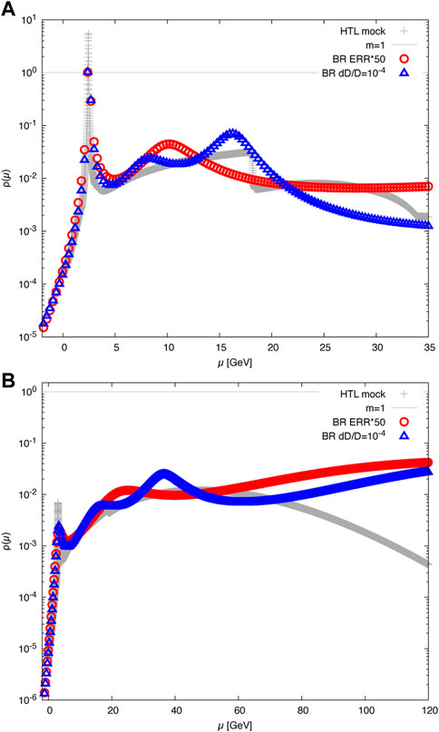
FIGURE 4. BR MAP reconstructions of the HTL Wilson loop spectral function (gray points) evaluated at T = 631 MeV and spatial separation distance r = 0.066 fm (A) and r = 0.264 fm (B). The reconstruction based on Nτ = 32 Euclidean data and a frequency range between μa ∈ [−5, 25] with Nω = 1,000 are shown as colored open symbols. The red data denotes the reconstruction based on the preconditioning ERRADAPTION = 50 while the final result exploting the full ΔD/D = 10−4 is given in blue.
5 New insight from machine learning
Over the past years interest in machine learning approaches to spectral function reconstruction has increased markedly (see also [128]). Several groups have put forward pioneering studies that explore how established machine learning strategies, such as supervised kernel ridge regression [129, 130], artificial neural networks [44, 45, 131–135] or Gaussian processes [136, 137] can be used to tackle the inverse problem in the context of extracting spectral functions from Euclidean lattice correlators. The machine learning mindset has already lead to new developments in the spectral reconstruction community, by providing new impulses to regularization of the ill-posed problem.
As a first step let us take a look at how machine learning strategies incorporate the necessary prior knowledge to obtain a unique answer to the reconstruction task. While in the Bayesian approach this information enters explicitly through the prior probability and its hyperparameters, it does so in the machine-learning context in three separate ways: To train supervised reconstruction algorithms a training dataset needs to be provided, often consisting of pairs of correlators and information on the encoded spectral functions. Usually a limited selection of relevant structures is included in this training data set, which amounts to prior knowledge on the spectrum. Both supervised and unsupervised machine learning is build around the concept of a cost- or optimization functional, which contains information on the provided data. It most often also features regulator terms, which can be of similar form as those discussed in Section 3.2. This in particular means that these regulators define the most probable values for the ρl’s in the absence of data and therefor take on a similar role as a Bayesian default model. The third entry point for prior knowledge lies in the choice of structures used to compose the machine learning model. In case that e.g. Gaussian processes are used, the choice of kernel of the common normal distribution for observed and unobserved data is based on prior knowledge, as is the selection of its hyperparameters. In case that neural networks are used, the number and structure of the deployed layers and activation functions similarly imprint additional prior information on the reconstructed spectral function, such as e.g., their positivity.
Direct applications of machine learning approaches developed in the context of image reconstruction to positive spectral function reconstruction have shown good performance on-par with Bayesian algorithms, such as the BR method or the MEM.
Can we understand why machine learning so far has not outpaced Bayesian approaches? One potential answer lies in the information scarcity of the input correlators themselves. If there is no unused information present in the correlator also sophisticated machine learning cannot go beyond what Bayesian approaches utilize. As shown in recent mock-data tests in the context of finite temperature hadron spectral functions in Ref. [67], increasing the number of available datapoints in imaginary time (i.e., going closer to the continuum limit) does not necessarily improve the reconstruction outcome significantly. One can see what is happening, when investigating the Matsubara frequency correlator, obtained from Euclidean input data via Fourier transform. As one decreases the temporal lattice spacing, the range of accessible high lying Matsubara frequencies increases but their coarseness, given by the inverse temperature of the system, remains the same. Of course formally all thermal real-time information can be reconstructed from access to the exact values of the (discrete) Matsubara frequency correlator. In practice, in the presence of finite errors, one finds that the in-medium correlator only at the lowest Matsubara frequencies shows significant changes compared to the T = 0 correlator and agrees with it within uncertainties at higher lying Matsubara frequencies. I.e. the contribution of thermal physics diminishes rapidly at higher Matsubara frequencies, which may in practice require increasingly smaller uncertainties on the input data for successful reconstruction at higher temperatures.
This information scarcity dilemma asks us to provide our reconstruction algorithms with more QCD specific prior information. So far the Bayesian priors have focused on very generic properties, such as positivity and smoothness. It is here that machine learning can and already has provided new impulses to the community.
One promising approach is to use neural networks as parametrization of spectral functions or parton distribution functions. First introduced in the context of PDFs in Ref. [45] and recently applied to the study of finite temperature spectra in Ref. [44] this approach allows to infuse the reconstruction with additional information about the analytic properties of ρ. Traditionally one would choose a specific parametrization apriori such as rational functions (Padé) or SVD basis functions (Bryan) and vary their parameters. The more versatile NN approach, thanks to the universal approximation theorem, allows us instead to explore different types of basis functions and assign an uncertainty to each choice.
The concept of learning can also be brought to the prior probability or regulator itself. Instead of constructing a regulator based on generic axioms, one may consider it as a neural network mapping the parameters ρl to a single penalty value P[ρ|I]. Training an optimal regulator within a Bayesian setting, based e.g., on realistic mock data, promises to capture more QCD specific properties than what is currently encoded in the BR or MEM. Exploring this path is work in progress.
6 Summary and conclusion
Progress in modern high-energy nuclear physics depends on first-principle knowledge of QCD dynamics, be it in the form of transport properties of quarks and gluons at high temperatures or the phase-space distributions of partons inside nucleons at low temperatures. Lattice QCD offers non-perturbative access to these quantities but due to its formulation in imaginary time, hides them behind an ill-posed inverse problem. The inverse problem is most succinctly stated in terms of a spectral decomposition, where the Euclidean correlator accessible on the lattice is expressed as integral over a spectral function multiplied by an analytic kernel. The real-time information of interest can often be read-off directly from the structures occurring in the spectral function. The determination of PDFs from the hadronic tensor and via pseudo PDFs can be formulated in terms of a similar inversion problem.
Bayesian inference provides a versatile tool set for the reconstruction of spectral functions. It gives meaning to the ill-posed inverse problem by incorporating relevant domain knowledge with an associated uncertainty budget through the prior probability distribution. Evaluating the posterior distribution, defined through Bayes theorem, gives access to the most probable values of the spectral function based on simulation data and prior knowledge. In addition it also encodes the full uncertainty budget through its spread. Traditionally predominantly MAP point estimates were computed due to lower computational cost of the corresponding optimization problem, compared to full Monte-Carlo sampling of the posterior. In that case information about the uncertainty budget is hidden from the user and it must be estimated manually. Several relevant challenges for uncertainty estimation in the lattice QCD context were discussed, including the problem of ringing and those related to comparing reconstructions based on different Euclidean time extents.
A brief user guide described how to run two open access codes accompanying this publication. One focuses on the determination of MAP point estimates based on the BR and MEM prior. The other utilizes a modern Monte-Carlo library to sample from the full BR posterior.
Last but not least a brief look is taken at machine learning approaches to spectral function reconstruction. The need for providing prior information is discussed and a common challenge among all reconstruction approaches, information scarcity in the input data, is pointed out. Two venues for combining the machine-learning viewpoint with the Bayesian strategy are touched upon.
With the concrete conceptual and technical discussions contained in this publication, the reader is equipped with a solid basis to carry out Bayesian spectral reconstructions. The provided open-access source codes offer a quick entry into the research field and can be modified according to different needs in regards to kernels arising in different lattice QCD studies.
Author contributions
AR: Conception, literature study, code development, writing, and editing.
Funding
Some of the spectral function reconstruction code has been developed in the context of the project NN9578K-QCDrtX “Real-time dynamics of nuclear matter under extreme conditions” funded by UNINETT Sigma2—the National Infrastructure for High Performance Computing and Data Storage in Norway. The author gladly acknowledges support by the Research Council of Norway under the FRIPRO Young Research Talent grant 286883.
Acknowledgments
The author thanks the referees for their valuable suggestions.
Conflict of interest
The author declares that the research was conducted in the absence of any commercial or financial relationships that could be construed as a potential conflict of interest.
Publisher’s note
All claims expressed in this article are solely those of the authors and do not necessarily represent those of their affiliated organizations, or those of the publisher, the editors and the reviewers. Any product that may be evaluated in this article, or claim that may be made by its manufacturer, is not guaranteed or endorsed by the publisher.
Footnotes
1This prior knowledge may be supplied by a quantum field theory such as QCD and QED but also from experiment.
2To avoid this complication, the BR regulator has been successfully combined with the arc-length penalty regulator in Ref. [67].
3A few works have explored stochastic strategies for the evaluation of the posterior in the context of the SOM [106] or the stochastic analytic continuation (SAI) method [107, 108], of which the MEM is a special limit [109].
4In lattice QCD it is often easier to collect more samples than to simulate on grids with more points along Euclidean time. Then at least the improvement of the reconstruction with increasing statistics needs to be considered.
5In cases where the kernel is temperature independent, e.g., for lattice effective field theory correlators, discarding large τ datapoints is equivalent to computing the reconstructed kernel.
References
1. Guenther JN. Overview of the QCD phase diagram: Recent progress from the lattice. Eur Phys J A (2021) 57(4):136. doi:10.1140/epja/s10050-021-00354-6
2. Fukushima K, Hatsuda T. The phase diagram of dense QCD. Rep Prog Phys (2011) 74:014001. doi:10.1088/0034-4885/74/1/014001
3. Borsanyi S, Fodor Z, Giordano M, Guenther JN, Katz SD, Pasztor A, Wong CH. Equation of state of a hot-and-dense quark gluon plasma: Lattice simulations at real μB vs. extrapolations (2022). arXiv:2208.05398.
4. Bazavov A, Ding HT, Hegde P, Kaczmarek O, Karsch F, Laermann E, et al. QCD equation of state to O(μB6) from lattice QCD. Phys Rev D (2017) 95(5):054504. doi:10.1103/PhysRevD.95.054504
5. Borsanyi S, Fodor Z, Guenther JN, Kara R, Parotto P, Pasztor A, et al. Resummed lattice QCD equation of state at finite baryon density: Strangeness neutrality and beyond. Phys Rev D (2022) 105(11):114504. doi:10.1103/PhysRevD.105.114504
6. Busza W, Rajagopal K, van der Schee W. Heavy ion collisions: The big picture, and the big questions. Annu Rev Nucl Part Sci (2018) 68:339–76. doi:10.1146/annurev-nucl-101917-020852
7. Kojo T. QCD equations of state and speed of sound in neutron stars. AAPPS Bull (2021) 31(1):11. doi:10.1007/s43673-021-00011-6
8. Pasechnik R, Šumbera M. Phenomenological review on quark–gluon plasma: Concepts vs. Observations. Universe (2017) 3(1):7. doi:10.3390/universe3010007
9. Bazavov A, Petreczky P, Weber JH. Equation of state in 2+1 flavor QCD at high temperatures. Phys Rev D (2018) 97(1):014510. doi:10.1103/PhysRevD.97.014510
10. Borsanyi S, Fodor Z, Guenther J, Kampert KH, Katz SD, Kawanai T, et al. Calculation of the axion mass based on high-temperature lattice quantum chromodynamics. Nature (2016) 539(7627):69–71. doi:10.1038/nature20115
11. Bazavov A, Bhattacharya T, DeTar C, Ding HT, Gottlieb S, Gupta R, et al. Equation of state in (2+1)-flavor QCD. Phys Rev D (2014) 90:094503. doi:10.1103/PhysRevD.90.094503
12. Burger F, Ilgenfritz EM, Lombardo MP, Müller-Preussker M. Equation of state of quark-gluon matter from lattice QCD with two flavors of twisted mass Wilson fermions. Phys Rev D (2015) 91(7):074504. doi:10.1103/PhysRevD.91.074504
13. Borsanyi S, Fodor Z, Hoelbling C, Katz SD, Krieg S, Szabo KK. Full result for the QCD equation of state with 2+1 flavors. Phys Lett B (2014) 730:99–104. doi:10.1016/j.physletb.2014.01.007
14. Jaiswal A, Roy V. Relativistic hydrodynamics in heavy-ion collisions: General aspects and recent developments. Adv High Energ Phys (2016) 2016:1–39. doi:10.1155/2016/9623034
15. Klein M, Yoshida R. Collider physics at HERA. Prog Part Nucl Phys (2008) 61:343–93. doi:10.1016/j.ppnp.2008.05.002
16. d’Enterria D, Kluth S, Zanderighi G, Ayala C, Benitez-Rathgeb MA, Bluemlein J, Boito D. The strong coupling constant: State of the art and the decade ahead (2022). arXiv:2203.08271.
17. Aoki Y, Blum T, Colangelo G, Collins S, Della Morte M, Dimopoulos P, et al. FLAG review 2021 (2021). arXiv:2111.09849.
18. Lin ZW, Ko CM, Li BA, Zhang B, Pal S. Multiphase transport model for relativistic heavy ion collisions. Phys Rev C (2005) 72:064901. doi:10.1103/PhysRevC.72.064901
19. Petersen H, Steinheimer J, Burau G, Bleicher M, Stöcker H. Fully integrated transport approach to heavy ion reactions with an intermediate hydrodynamic stage. Phys Rev C (2008) 78:044901. doi:10.1103/PhysRevC.78.044901
20. Bratkovskaya EL, Cassing W, Konchakovski VP, Linnyk O. Parton-hadron-string dynamics at relativistic collider energies. Nucl Phys A (2011) 856:162–82. doi:10.1016/j.nuclphysa.2011.03.003
21. Cao S, Wang XN. Jet quenching and medium response in high-energy heavy-ion collisions: A review. Rep Prog Phys (2021) 84(2):024301. doi:10.1088/1361-6633/abc22b
22. Rothkopf A. Heavy quarkonium in extreme conditions. Phys Rep (2020) 858:1–117. doi:10.1016/j.physrep.2020.02.006
23. Abdul Khalek R, D'Alesio U, Arratia M, Bacchetta A, Battaglieri M, Begel M, et al. Snowmass 2021 white paper: Electron ion collider for high energy physics. In: 2022 snowmass summer study (2022). 2203.13199.
24. Alexandrou C, Bacchio S, Constantinou M, Finkenrath J, Hadjiyiannakou K, Jansen K, et al. Complete flavor decomposition of the spin and momentum fraction of the proton using lattice QCD simulations at physical pion mass. Phys Rev D (2020) 101(9):094513. doi:10.1103/PhysRevD.101.094513
25. Wang G, Yang YB, Liang J, Draper T, Liu KF. Proton momentum and angular momentum decompositions with overlap fermions. Phys Rev D (2022) 106(1):014512. doi:10.1103/PhysRevD.106.014512
26. Meissner S, Metz A, Schlegel M. Generalized parton correlation functions for a spin-1/2 hadron. J High Energ Phys (2009) 08:056. doi:10.1088/1126-6708/2009/08/056
27. Constantinou M, Debbio LD, Ji X, Lin HW, Liu KF, Monahan C, et al. Lattice QCD calculations of parton physics (2022). arXiv:2202.07193.
28. Ji X. Parton physics on a euclidean lattice. Phys Rev Lett (2013) 110:262002. doi:10.1103/PhysRevLett.110.262002
29. Radyushkin AV. Quasi-parton distribution functions, momentum distributions, and pseudo-parton distribution functions. Phys Rev D (2017) 96(3):034025. doi:10.1103/PhysRevD.96.034025
30. Liu KF, Dong SJ. Origin of difference betweenu¯ andd¯ partons in the nucleon. Phys Rev Lett (1994) 72:1790–3. doi:10.1103/PhysRevLett.72.1790
31. Schwartz MD. Quantum field theory and the standard model. Cambridge: Cambridge University Press (2014).
32. Dupuis N, Canet L, Eichhorn A, Metzner W, Pawlowski JM, Tissier M, et al. The nonperturbative functional renormalization group and its applications. Phys Rep (2021) 910:1–114. doi:10.1016/j.physrep.2021.01.001
33. Blaizot JP, Pawlowski JM, Reinosa U. Functional renormalization group and 2PI effective action formalism. Ann Phys (N Y) (2021) 431:168549. doi:10.1016/j.aop.2021.168549
34. Fischer CS. Infrared properties of qcd from dyson–schwinger equations. J Phys G: Nucl Part Phys (2006) 32(8):253–91. doi:10.1088/0954-3899/32/8/r02
35. Roberts CD. Strong QCD and dyson-schwinger equations. IRMA Lect Math Theor Phys (2015) 21:355–458. 1203.5341.
36. Montvay I, Münster G. Quantum fields on a lattice. Cambridge: Cambridge Monographs on Mathematical Physics. Cambridge University Press (1994).
37. Gattringer C, Lang CB. Quantum chromodynamics on the lattice vol. 788. Berlin: Springer (2010). doi:10.1007/978-3-642-01850-3
38. Gattringer C, Langfeld K. Approaches to the sign problem in lattice field theory. Int J Mod Phys A (2016) 31(22):1643007. doi:10.1142/S0217751X16430077
39. Berger CE, Rammelmüller L, Loheac AC, Ehmann F, Braun J, Drut JE. Complex Langevin and other approaches to the sign problem in quantum many-body physics. Phys Rep (2021) 892:1–54. doi:10.1016/j.physrep.2020.09.002
40. Bellac ML. Thermal field theory. Cambridge: Cambridge Monographs on Mathematical Physics. Cambridge University Press (2011). doi:10.1017/CBO9780511721700
41. Ghiglieri J, Kurkela A, Strickland M, Vuorinen A. Perturbative thermal QCD: Formalism and applications. Phys Rep (2020) 880:1–73. doi:10.1016/j.physrep.2020.07.004
42. Meyer HB. Transport properties of the quark-gluon plasma: A lattice QCD perspective. Eur Phys J A (2011) 47:86. doi:10.1140/epja/i2011-11086-3
43. Hadamard J. Sur les problèmes aux dérivées partielles et leur signification physique. Princeton, NJ, USA: Princeton university bulletin (1902). p. 49–52.
44. Shi S, Wang L, Zhou K. Rethinking the ill-posedness of the spectral function reconstruction - why is it fundamentally hard and how Artificial Neural Networks can help (2022). arXiv:2201.02564.
45. Karpie J, Orginos K, Rothkopf A, Zafeiropoulos S. Reconstructing parton distribution functions from Ioffe time data: From bayesian methods to neural networks. J High Energ Phys (2019) 04:057. doi:10.1007/JHEP04(2019)057
46. Nakahara Y, Asakawa M, Hatsuda T. Hadronic spectral functions in lattice QCD. Phys Rev D (1999) 60:091503. doi:10.1103/PhysRevD.60.091503
47. Asakawa M, Hatsuda T, Nakahara Y. Maximum entropy analysis of the spectral functions in lattice QCD. Prog Part Nucl Phys (2001) 46:459–508. doi:10.1016/S0146-6410(01)00150-8
48. Jarrell M, Gubernatis JE. Bayesian inference and the analytic continuation of imaginary-time quantum Monte Carlo data. Phys Rep (1996) 269(3):133–95. doi:10.1016/0370-1573(95)00074-7
49. Skilling J, Gull SF. Bayesian maximum entropy image reconstruction. Lecture Notes-Monograph Ser (1991) 1991:341–67.
50. Yamazaki T, Aoki S, Burkhalter R, Fukugita M, Hashimoto S, Ishizuka N, et al. Spectral function and excited states in lattice qcd with the maximum entropy method. Phys Rev D (2001) 65:014501. doi:10.1103/PhysRevD.65.014501
51. Sasaki K, Sasaki S, Hatsuda T. Spectral analysis of excited nucleons in lattice qcd with maximum entropy method. Phys Lett B (2005) 623(3):208–17. doi:10.1016/j.physletb.2005.07.026
52. Fiebig HR. Spectral density analysis of time correlation functions in lattice qcd using the maximum entropy method. Phys Rev D (2002) 65:094512. doi:10.1103/PhysRevD.65.094512
53. Liang J, Draper T, Liu KF, Rothkopf A, Yang YB. Towards the nucleon hadronic tensor from lattice QCD. Phys Rev D (2020) 101(11):114503. doi:10.1103/PhysRevD.101.114503
54. Asakawa M, Hatsuda T. J/ψandηcin the deconfined plasma from lattice QCD. Phys Rev Lett (2004) 92:012001. doi:10.1103/PhysRevLett.92.012001
55. Datta S, Karsch F, Petreczky P, Wetzorke I. Behavior of charmonium systems after deconfinement. Phys Rev D (2004) 69:094507. doi:10.1103/PhysRevD.69.094507
56. Umeda T, Nomura K, Matsufuru H. Charmonium at finite temperature in quenched lattice QCD. Eur Phys J C (2005) 39S1:9–26. doi:10.1140/epjcd/s2004-01-002-1
57. Jakovac A, Petreczky P, Petrov K, Velytsky A. Quarkonium correlators and spectral functions at zero and finite temperature. Phys Rev D (2007) 75:014506. doi:10.1103/PhysRevD.75.014506
58. Aarts G, Allton C, Kim S, Lombardo MP, Oktay MB, Ryan SM, et al. What happens to the ϒ and ηb in the quark-gluon plasma? Bottomonium spectral functions from lattice QCD. J High Energ Phys (2011) 11:103. doi:10.1007/JHEP11(2011)103
59. Aarts G, Allton C, Kim S, Lombardo MP, Oktay MB, Ryan SM, et al. S wave bottomonium states moving in a quark-gluon plasma from lattice NRQCD. J High Energ Phys (2013) 03:084. doi:10.1007/JHEP03(2013)084
60. Ding HT, Francis A, Kaczmarek O, Karsch F, Satz H, Soeldner W. Charmonium properties in hot quenched lattice QCD. Phys Rev D (2012) 86:014509. doi:10.1103/PhysRevD.86.014509
61. Aarts G, Allton C, Kim S, Lombardo MP, Ryan SM, Skullerud JI. Melting of P wave bottomonium states in the quark-gluon plasma from lattice NRQCD. J High Energ Phys (2013) 12:064. doi:10.1007/JHEP12(2013)064
62. Aarts G, Allton C, Harris T, Kim S, Lombardo MP, Ryan SM, et al. The bottomonium spectrum at finite temperature from Nf = 2 + 1 lattice QCD. J High Energ Phys (2014) 07:097. doi:10.1007/JHEP07(2014)097
63. Borsanyi S, Durr S, Fodor Z, Hoelbling C, Katz SD, Krieg S, et al. Charmonium spectral functions from 2+1 flavour lattice QCD. J High Energ Phys (2014) 04:132. doi:10.1007/jhep04(2014)132
64. Kim S, Petreczky P, Rothkopf A. Lattice NRQCD study of S- and P-wave bottomonium states in a thermal medium with Nf = 2 + 1 light flavors. Phys Rev D (2015) 91:054511. doi:10.1103/PhysRevD.91.054511
65. Ikeda A, Asakawa M, Kitazawa M. In-medium dispersion relations of charmonia studied by the maximum entropy method. Phys Rev D (2017) 95(1):014504. doi:10.1103/PhysRevD.95.014504
66. Kelly A, Rothkopf A, Skullerud JI. Bayesian study of relativistic open and hidden charm in anisotropic lattice QCD. Phys Rev D (2018) 97(11):114509. doi:10.1103/PhysRevD.97.114509
67. Kim S, Petreczky P, Rothkopf A. Quarkonium in-medium properties from realistic lattice NRQCD. J High Energ Phys (2018) 11:088. doi:10.1007/JHEP11(2018)088
68. Gubler P, Morita K, Oka M. Charmonium spectra at finite temperature from QCD sum rules with the maximum entropy method. Phys Rev Lett (2011) 107:092003. doi:10.1103/PhysRevLett.107.092003
69. Araki KJ, Ohtani K, Gubler P, Oka M. QCD sum rules on the complex Borel plane. Prog Theor Exp Phys (2014) 2014:73B03–0. doi:10.1093/ptep/ptu092
70. Meyer HB. Calculation of the shear viscosity in SU(3) gluodynamics. Phys Rev D (2007) 76:101701. doi:10.1103/PhysRevD.76.101701
71. Meyer HB. Calculation of the bulk viscosity in SU(3) gluodynamics. Phys Rev Lett (2008) 100:162001. doi:10.1103/PhysRevLett.100.162001
72. Aarts G, Allton C, Foley J, Hands S, Kim S. Spectral functions at small energies and the electrical conductivity in hot, quenched lattice QCD. Phys Rev Lett (2007) 99:022002. doi:10.1103/PhysRevLett.99.022002
73. Ding HT, Francis A, Kaczmarek O, Karsch F, Laermann E, Soeldner W. Thermal dilepton rate and electrical conductivity: An analysis of vector current correlation functions in quenched lattice QCD. Phys Rev D (2011) 83:034504. doi:10.1103/PhysRevD.83.034504
74. Aarts G, Allton C, Amato A, Giudice P, Hands S, Skullerud JI. Electrical conductivity and charge diffusion in thermal QCD from the lattice. J High Energ Phys (2015) 02:186. doi:10.1007/JHEP02(2015)186
75. Amato A, Aarts G, Allton C, Giudice P, Hands S, Skullerud JI. Electrical conductivity of the quark-gluon plasma across the deconfinement transition. Phys Rev Lett (2013) 111(17):172001. doi:10.1103/PhysRevLett.111.172001
76. Astrakhantsev N, Braguta V, Kotov A. Temperature dependence of shear viscosity of SU(3)–gluodynamics within lattice simulation. J High Energ Phys (2017) 04:101. doi:10.1007/JHEP04(2017)101
77. Rothkopf A, Hatsuda T, Sasaki S. Complex heavy-quark potential at finite temperature from lattice QCD. Phys Rev Lett (2012) 108:162001. doi:10.1103/PhysRevLett.108.162001
78. Burnier Y, Kaczmarek O, Rothkopf A. Static quark-antiquark potential in the quark-gluon plasma from lattice QCD. Phys Rev Lett (2015) 114(8):082001. doi:10.1103/PhysRevLett.114.082001
79. Burnier Y, Kaczmarek O, Rothkopf A. Quarkonium at finite temperature: Towards realistic phenomenology from first principles. J High Energ Phys (2015) 12:101–34. doi:10.1007/JHEP12(2015)101
80. Burnier Y, Rothkopf A. Complex heavy-quark potential and Debye mass in a gluonic medium from lattice QCD. Phys Rev D (2017) 95(5):054511. doi:10.1103/PhysRevD.95.054511
81. Dudal D, Oliveira O, Silva PJ. Källén-Lehmann spectroscopy for (un)physical degrees of freedom. Phys Rev D (2014) 89(1):014010. doi:10.1103/PhysRevD.89.014010
82. Ilgenfritz EM, Pawlowski JM, Rothkopf A, Trunin A. Finite temperature gluon spectral functions from Nf = 2 + 1 + 1 lattice QCD. Eur Phys J C (2018) 78(2):127. doi:10.1140/epjc/s10052-018-5593-7
83. Dudal D, Oliveira O, Roelfs M, Silva P. Spectral representation of lattice gluon and ghost propagators at zero temperature. Nucl Phys B (2020) 952:114912. doi:10.1016/j.nuclphysb.2019.114912
84. Lepage GP, Clark B, Davies CTH, Hornbostel K, Mackenzie PB, Morningstar C, et al. Constrained curve fitting. Nucl Phys B - Proc Supplements (2002) 106:12–20. doi:10.1016/S0920-5632(01)01638-3
85. Burnier Y, Ding HT, Kaczmarek O, Kruse AL, Laine M, Ohno H, et al. Thermal quarkonium physics in the pseudoscalar channel. J High Energ Phys (2017) 11:206. doi:10.1007/JHEP11(2017)206
86. McElreath R. Statistical rethinking: A bayesian course with examples in R and stan. 2nd ed. Boca Raton, FL, USA: CRC Press (2020).
87. Bishop CM. Pattern recognition and machine learning (information science and statistics). Berlin, Heidelberg: Springer (2006).
88. Endres MG, Kaplan DB, Lee JW, Nicholson AN. Listening to noise. PoS LATTICE (2011) 2011:017. doi:10.22323/1.139.0017
89. DeGrand T. Log-normal distribution for correlators in lattice QCD? Phys Rev D (2012) 86:014512. doi:10.1103/PhysRevD.86.014512
90. Efron B, Tibshirani RJ. An introduction to the bootstrap. Monographs on statistics and applied probability, vol. 57. Boca Raton, Florida, USA: Chapman & Hall/CRC (1993).
91. Cyrol AK, Pawlowski JM, Rothkopf A, Wink N. Reconstructing the gluon. Scipost Phys (2018) 5(6):065. doi:10.21468/SciPostPhys.5.6.065
92. Binosi D, Tripolt RA. Spectral functions of confined particles. Phys Lett B (2020) 801:135171. doi:10.1016/j.physletb.2019.135171
94. Rudin LI, Osher S, Fatemi E. Nonlinear total variation based noise removal algorithms. Physica D: Nonlinear Phenomena (1992) 60(1-4):259–68. doi:10.1016/0167-2789(92)90242-F
95. Bardsley JM. Laplace-distributed increments, the laplace prior, and edge-preserving regularization. J Inverse Ill-Posed Probl (2012) 20(3):271–85. doi:10.1515/jip-2012-0017
96. Fischer CS, Pawlowski JM, Rothkopf A, Welzbacher CA. Bayesian analysis of quark spectral properties from the Dyson-Schwinger equation. Phys Rev D (2018) 98(1):014009. doi:10.1103/PhysRevD.98.014009
97.Event Horizon Telescope Collaboration, Akiyama K, Alberdi A, Alef W, Asada K, Azulay R, et al. First M87 event horizon telescope results. I. The shadow of the supermassive black hole. Astrophys J (2019) 875(1):1. doi:10.3847/2041-8213/ab0ec7
98. Narayan R, Nityananda R. Maximum entropy image restoration in astronomy. Annu Rev Astron Astrophys (1986) 24(1):127–70. doi:10.1146/annurev.aa.24.090186.001015
99. Skilling J. The axioms of maximum entropy. In: Maximum-entropy and bayesian methods in science and engineering. Berlin: Springer (1988). p. 173–87.
100. Burnier Y, Rothkopf A. Bayesian approach to spectral function reconstruction for euclidean quantum field theories. Phys Rev Lett (2013) 111:182003. doi:10.1103/PhysRevLett.111.182003
101. Harris T, Meyer HB, Robaina D. A variational method for spectral functions. PoS LATTICE (2016) 2016:339. doi:10.22323/1.256.0339
102. Bala D, Kaczmarek O, Larsen R, Mukherjee S, Parkar G, Petreczky P, et al. Static quark-antiquark interactions at nonzero temperature from lattice QCD. Phys Rev D (2022) 105(5):054513. doi:10.1103/PhysRevD.105.054513
103. Hobson M, Lasenby A. The entropic prior for distributions with positive and negative values. Mon Not R Astron Soc (1998) 298:905–8. doi:10.1046/j.1365-8711.1998.01707.x
104. Rothkopf A. Bayesian inference of nonpositive spectral functions in quantum field theory. Phys Rev D (2017) 95(5):056016. doi:10.1103/PhysRevD.95.056016
105. Haas M, Fister L, Pawlowski JM. Gluon spectral functions and transport coefficients in Yang–Mills theory. Phys Rev D (2014) 90:091501. doi:10.1103/PhysRevD.90.091501
106. Mishchenko A, Prokof’Ev N, Sakamoto A, Svistunov B. Diagrammatic quantum Monte Carlo study of the fröhlich polaron. Phys Rev B (2000) 62(10):6317–36. doi:10.1103/physrevb.62.6317
107. Ding HT, Kaczmarek O, Mukherjee S, Ohno H, Shu HT. Stochastic reconstructions of spectral functions: Application to lattice qcd. Phys Rev D (2018) 97(9):094503. doi:10.1103/physrevd.97.094503
108. Shao H, Sandvik AW. Progress on stochastic analytic continuation of quantum Monte Carlo data (2022). arXiv:2202.09870.
109. Beach K. Identifying the maximum entropy method as a special limit of stochastic analytic continuation (2004). arXiv preprint cond-mat/0403055.
110. Press WH, Teukolsky SA, Vetterling WT, Flannery BP. Numerical recipes 3rd edition: The art of scientific computing. 3rd ed. Cambridge: Cambridge University Press (2007).
111. Burnier Y, Laine M, Mether L. A Test on analytic continuation of thermal imaginary-time data. Eur Phys J C (2011) 71:1619. doi:10.1140/epjc/s10052-011-1619-0
112. Zhu Y, Vuorinen A. The shear channel spectral function in hot Yang-Mills theory. J High Energ Phys (2013) 03:002. doi:10.1007/JHEP03(2013)002
113. Burnier Y, Laine M. Massive vector current correlator in thermal QCD. J High Energ Phys (2012) 11:086. doi:10.1007/JHEP11(2012)086
114. Vuorinen A, Zhu Y. On the infrared behavior of the shear spectral function in hot Yang-Mills theory. J High Energ Phys (2015) 03:138. doi:10.1007/JHEP03(2015)138
115. Jeffreys H. An invariant form for the prior probability in estimation problems. Proc R Soc Lond A Math Phys Sci (1946) 186(1007):453–61. doi:10.1098/rspa.1946.0056
116. Bryan RK. Maximum entropy analysis of oversampled data problems. Eur Biophys J (1990) 18(3):165–74. doi:10.1007/BF02427376
117. Rothkopf A. Improved maximum entropy analysis with an extended search space. J Comput Phys (2013) 238:106–14. doi:10.1016/j.jcp.2012.12.023
118. Rothkopf A. Improved maximum entropy method with extended search space. PoS LATTICE (2012) 2012:100. doi:10.22323/1.164.0100
119. Rothkopf A. MAP Implementation of the BR method & MEM. Zenodo (2022). doi:10.5281/zenodo.7362890
121. Granlund T. The GMP development team: GNU MP: The GNU multiple precision arithmetic library, 5.0.5 edn. (2012).
122. Fousse L, Hanrot G, Lefèvre V, Pélissier P, Zimmermann P. Mpfr: A multiple-precision binary floating-point library with correct rounding. ACM Trans Math Softw (2007) 33(2):13. doi:10.1145/1236463.1236468
123. Ding HT, Kaczmarek O, Karsch F, Satz H, Soldner W. Charmonium correlators and spectral functions at finite temperature. PoS LAT (2009) 2009:169. doi:10.22323/1.091.0169
124. Malouf R. A comparison of algorithms for maximum entropy parameter estimation. In: Proceedings of the 6th Conference on Natural Language Learning - Volume 20. COLING-02. Stroudsburg, Pennsylvania, USA: Association for Computational Linguistics (2002). p. 1–7. doi:10.3115/1118853.1118871
125. Carpenter B, Gelman A, Hoffman MD, Lee D, Goodrich B, Betancourt M, et al. Stan: A probabilistic programming language. J Stat Softw (2017) 76(1). doi:10.18637/jss.v076.i01
127. Burnier Y, Rothkopf A. Hard thermal loop benchmark for the extraction of the nonperturbative QQ¯ potential. Phys Rev D (2013) 87:114019. doi:10.1103/PhysRevD.87.114019
128. Boyda D, Calì S, Foreman S, Funcke L, Hackett DC, Lin Y, et al. Applications of machine learning to lattice quantum field theory. In: 2022 snowmass summer study (2022). 2202.05838.
129. Offler S, Aarts G, Allton C, Jäger B, Kim S, Lombardo MP, et al. Reconstruction of bottomonium spectral functions in thermal QCD using Kernel Ridge Regression. PoS LATTICE (2022) 2021:509. doi:10.22323/1.396.0509
130. Spriggs T, Aarts G, Allton C, Burns T, Horohan D’Arcy R, Jager B, et al. A comparison of spectral reconstruction methods applied to non-zero temperature NRQCD meson correlation functions. EPJ Web Conf (2022) 258:05011. doi:10.1051/epjconf/202225805011
131. Fournier R, Wang L, Yazyev OV, Wu Q. Artificial neural network approach to the analytic continuation problem. Phys Rev Lett (2020) 124(5):056401. doi:10.1103/physrevlett.124.056401
132. Kades L, Pawlowski JM, Rothkopf A, Scherzer M, Urban JM, Wetzel SJ, et al. Spectral reconstruction with deep neural networks. Phys Rev D (2020) 102(9):096001. doi:10.1103/PhysRevD.102.096001
133. Chen SY, Ding HT, Liu FY, Papp G, Yang CB. Machine learning spectral functions in lattice QCD (2021). arXiv:2110.13521.
134. Wang L, Shi S, Zhou K. Automatic differentiation approach for reconstructing spectral functions with neural networks. In: 35th conference on neural information processing systems (2021). 2112.06206.
135. Lechien T, Dudal D. Neural network approach to reconstructing spectral functions and complex poles of confined particles. Scipost Phys (2022) 13(4):097. doi:10.21468/SciPostPhys.13.4.097
136. Valentine AP, Sambridge M. Gaussian process models—I. A framework for probabilistic continuous inverse theory. Geophys J Int (2020) 220(3):1632–47. doi:10.1093/gji/ggz520
Keywords: Bayesian inference, lattice QCD, spectral functions, strong interaction, inverse problem
Citation: Rothkopf A (2022) Bayesian inference of real-time dynamics from lattice QCD. Front. Phys. 10:1028995. doi: 10.3389/fphy.2022.1028995
Received: 26 August 2022; Accepted: 25 November 2022;
Published: 14 December 2022.
Edited by:
Evgeny Epelbaum, Ruhr University Bochum, GermanyReviewed by:
Attila Pásztor, Eötvös Loránd University, HungaryJon-Ivar Skullerud, Maynooth University, Ireland
Copyright © 2022 Rothkopf. This is an open-access article distributed under the terms of the Creative Commons Attribution License (CC BY). The use, distribution or reproduction in other forums is permitted, provided the original author(s) and the copyright owner(s) are credited and that the original publication in this journal is cited, in accordance with accepted academic practice. No use, distribution or reproduction is permitted which does not comply with these terms.
*Correspondence: Alexander Rothkopf, alexander.rothkopf@uis.no