Research on laser center positioning under CV model segmentation

Spot positioning accuracy is an important index of laser processing system and ranging system. When the laser spot is noisy or the gray level is not uniform, the positioning accuracy is easily affected. Aiming at the above problems, this paper proposes a laser spot segmentation method based on the Chan-Vese model, which can improve the accuracy of spot center localization in combination with the gray centroid method. Firstly, the laser spot image is decomposed by two-dimensional wavelet, and the high-frequency component is suppressed by soft threshold function to eliminate the noise in the laser spot image. Secondly, the level set algorithm based on Chan-Vese model is used to segment the laser spot image with adaptive improvement of the initial coordinates of the evolution curve. Finally, the center coordinates are calculated inside the segmentation curve using the gray centroid method. Experimental results show that the method is more accurate and robust.

Introduction

Laser has many advantages, such as energy concentration, good directivity and low divergence, etc. It is widely used in machining, guidance, ranging and other fields. Laser spot location is the key technology of the whole system, so many algorithms are proposed [1]. The common methods to detect the center of laser spot include the Hough transform method [2], the circular fitting method [3], and the gray centroid method [4], Hough transform is a feature detection method proposed by Hough in 1962. It can detect the shape of the image by constructing functions to describe the edge pixels [5]. The Hough transform is required to vote-by-point, which accuracy is only of pixel level [6]. The circle fitting method is to use the least squares to fit the geometric features of the image, which is easily affected by the noise [3]. The gray centroid method needs to use the light intensity received by each pixel on the two-dimensional image, and requires high uniformity of the laser spot brightness [7]. In order to improve the positioning accuracy, many improved algorithms have been proposed in recent years. Liu et al. proposed a curve fitting sub-pixel location algorithm of barycenter, only few data points are calculated by the algorithm which meets the accuracy requirements of micro distortion measurement [8], The algorithm is more suitable for laser spot image of Gauss Distribution. Jiang et al put forward a nonlinear least square fitting algorithm to compensate the system error, so as to improve the positioning accuracy of gray centroid method [9]. Liu et al used an algorithm based on the optimal arc to obtain the center for the laser spot by fitting the circle center [10]. It is found that image denoising and laser spot boundary location are important prerequisites for measuring the center position of laser spot, so we focuses on laser spot denoising and image segmentation [11, 12].

In this paper, combining with the gray centroid method, the proposed laser spot segmentation method based on Chan-Vese [13] model can further improve the accuracy of laser spot positioning. The image is pre-processed by wavelet decomposition and reconstruction to solve the problem of uneven gray scale of the image and reduce the interference of noise on the contour. The laser spot boundary is calculated using the level set method based on the CV model. The grayscale center of mass is calculated within the closed shape to obtain the exact center coordinates. The method is fully validated in experiments.

Theoretical analysis

Wavelet decomposition denoising

Wavelet transform is a local transform of space and frequency, which can separate noise information from signal effectively [14]. The 2D discrete wavelet decomposition and reconstruction of the image can be represented as Figure 1. First, perform one-dimensional discrete wavelet transform and down-sampling on the row direction of the image, so as to calculate the low-frequency component L and high-frequency component H of the image in the row direction. Repeat the above process in column direction, finally get the four subgraphs A, H, V, D. A represents the low frequency part of the image, H, V, D represent the high-frequency parts of the image in the horizontal, vertical, and diagonal directions, respectively. The low-frequency sub-image reflects the overall information of the image, and the high-frequency sub-images reflect the local details of the image [15, 16]. Continue to repeat the process of Figure 2 for the low-frequency sub-images, that is, to obtain the multi-layer wavelet decomposition of the image.

FIGURE 1

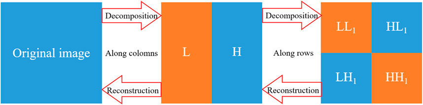
FIGURE 1. Discrete wavelet decomposition and reconstruction of images.

FIGURE 2

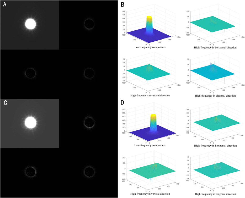
FIGURE 2. Wavelet Decomposition Results and Wavelet Coefficient Distribution of Laser Spot Image. (A): The first layer of wavelet decomposition; (B): The first layer of wavelet coefficient distribution; (C): The second layer of wavelet decomposition; (D): The second layer of wavelet coefficient distribution.

In this paper, two-layer wavelet decomposition is performed on the laser spot image, and the process can be expressed as Figure 2. After image wavelet decomposition, the image noise is reflected in the high-frequency components, and the absolute value of the wavelet coefficient is small; while the part with uniform laser energy is reflected in the high-frequency component, and the wavelet coefficient is large. According to the idea of wavelet threshold denoising proposed by John Stone [17], when the wavelet coefficient is less than a certain threshold, it is considered to be mainly noise components, and the part larger than the threshold is retained.

We chose the VisuShrink [17] method to generate the threshold, the formula is

$T=\sigma \sqrt{2\mathrm{l}\mathrm{g}N}(1)$

where σ is the image standard deviation and N is the image size. Generally, the threshold function is divided into two types: hard threshold function and soft threshold function. Because the hard threshold function is prone to Ringingeffect [18], We chooses the soft threshold method to process the estimated wavelet coefficients, which can be expressed as:

${\stackrel{⌢}{w}}_{j,k}=\{\begin{array}{cc}sign\left(w_{j,k}\right)\left(\left|w_{j,k}\right|-T\right),& \left|w_{j,k}\right|\ge T\\ 0,& \left|w_{j,k}\right|<T\end{array}(2)$

Where: sign (*) is the sign function, $w_{j,k}$is the wavelet coefficient before processing, ${\stackrel{⌢}{w}}_{j,k}$ is the wavelet coefficient after processing. The threshold T is given by Eq. 1.

Figure 3 shows the comparison effect of the spot image before and after denoising. After denoising, the edge high-frequency noise texture and radial light are better suppressed, and the image Grayscale Value image is smoother.

FIGURE 3

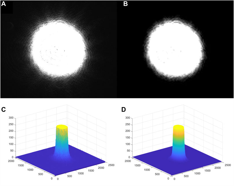
FIGURE 3. Comparison of before and after laser spot image denoising. (A): Image before denoising; (B): Image after denoising; (C): Grayscale Value distribution before denoising; (D): Grayscale Value distribution after denoising.

Laser spot segmentation based on CV model

This section will discuss the applicability of the CV model to laser spot segmentation. The key of the CV model is to use the image grayscale information to construct the energy function E(C), so as to evolve the curve to a certain target area. The energy function can be expressed as

$\begin{array}{l}{E}^{cv}\left(c_1,c_2,C\right)=\mu \cdot Length\left(C\right)+{\lambda }_1\cdot {\underset{inside\left(C\right)}{{\displaystyle \int }}\left|u_0\left(x,y\right)-c_1\right|}^{2}dxdy\\ +{\lambda }_2\cdot {\underset{outside\left(C\right)}{{\displaystyle \int }}\left|u_0\left(x,y\right)-c_2\right|}^{2}dxdy\end{array}(3)$

Where, μ is the length weight of the contour line; C is the contour line of the target, u is the target image; and λ₁ and λ₂ are the correction weights; c₁ and c₂ are the mean image gray levels inside and outside the evolution curve C, respectively. The formula is divided into three items; the first item is the regularization item, which is used to constrain the length of the contour line to ensure that the contour line is the shortest under the current conditions; the second and third items are the contour line condition items, which are responsible for controlling the current contour line evolution trend. Use level set functions to control curve evolution, The level set function is expressed as

$\phi \left(x,y\right)\{\begin{array}{cc}>0;& x,y\in inside\left(C\right)\\ =0;& x,y\in boundary\left(C\right)\\ <0;& x,y\in outside\left(C\right)\end{array}(4)$

Eq. 4 is substituted into Eq. 3. Also, the energy function E(C) is be written as

$\begin{array}{l}{E}^{cv}(c_1,c_2,\phi )=\mu \cdot \underset{\mathrm{\Omega }}{{\displaystyle \int }}{\delta }_{\epsilon }(\phi (x,y))\left|\nabla \phi \left(x,y\right)\right|dxdy\\ +{\lambda }_1\cdot {\underset{\mathrm{\Omega }}{{\displaystyle \int }}\left|u_0\left(x,y\right)-c_1\right|}^2{H}_{\epsilon }\left(\phi \left(x,y\right)\right)dxdy\\ +{\lambda }_2\cdot {\underset{\mathrm{\Omega }}{{\displaystyle \int }}\left|u_0\left(x,y\right)-c_2\right|}^2\left(1-H_{\epsilon }\left(\phi \left(x,y\right)\right)\right)dxdy\end{array}(5)$

H_ε is Heaviside Function, Use its approximate form

$H_{\epsilon }\left(z\right)=\frac{1}{2}\left(1+\frac{2}{\pi }\arctan \left(\frac{z}{\epsilon }\right)\right)(6)$

${\delta }_{\epsilon }\left(z\right)=\frac{1}{\pi }\cdot \frac{\epsilon }{{\epsilon }^2+{\pi }^2}(7)$

The minimization problem is solved by solving the Euler-Lagrange equation corresponding to Eq. 5. Using Variation and Gradient Descent to Solve the Extreme Values of Energy Functionals, as in Eq. 8. Finally, the energy equation evolution curve is obtained.

$\frac{\partial \phi }{\partial t}=\delta \left(\phi \right)\left[\mu div\left(\frac{\nabla \phi }{\left|\nabla \phi \right|}\right)-{\lambda }_1{\left(u-c_1\right)}^2+{\lambda }_2{\left(u-c_2\right)}^2\right](8)$

In order to speed up the evolution process, optimize the initial position of the level set function, Compute the global image grayscale centroid. Obviously the center of mass coordinates are inside the laser spot. This is a rough estimate and cannot be used for precise positioning, But it is enough to make the level set function get a suitable initial position, so that the gradient descent is faster.

In Figure 4A, the laser spot positions are different, but the initial curve positions of the level set algorithm are all inside the spot. The curve evolution results are shown in Figure 4B. The image is segmented according to the closed curve, and the grayscale center of mass is calculated again for the interior of the curve to obtain a more accurate center position.

FIGURE 4

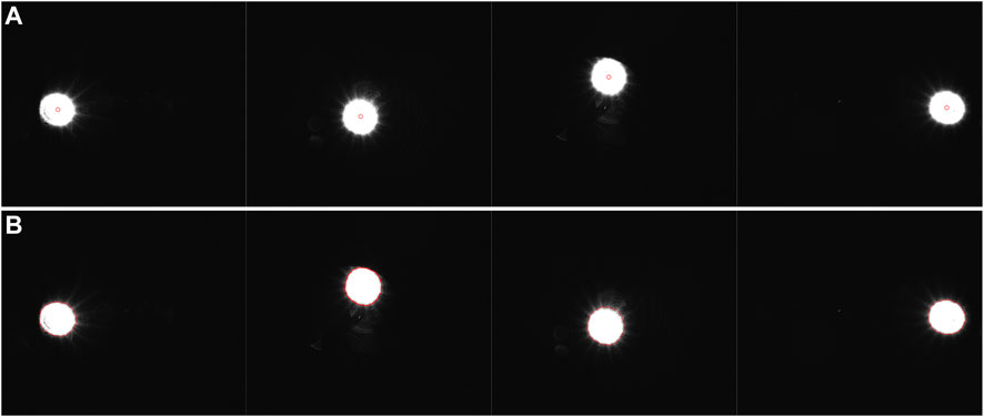
FIGURE 4. Adaptive initial curve coordinates and evolutionary results. (A): Images of laser spot at different positions; (B): Fitting results of laser spot images at different positions.

Experiment and analysis

In this section, we design several sets of experiments and compare our method with the Hough transform method, the circular fitting method, and the grayscale center-of-mass method. The data used in the experiment comes from the real laser spot image we collected, in which the laser model is MSL-FN-532 and the size of the CCD camera is 2456 × 2048 pixels, The shooting is done on an optical platform.

Experimental data

Since the real data do not have a priori coordinate position information, we designed five sets of experiments to verify the performance of the algorithm. The experimental images are shown in Figure 5. When taking the first three sets of images, the laser and the camera remain relatively fixed. The first group contains nine pictures, taken at different time points; The second group contains nine pictures, and the laser spot has different sizes by adjusting the beam expander; The third group contains five images, and by changing the attenuation ratio, laser spots of different powers are generated; The fourth group contains 8 images, with the laser moving horizontally as they were taken; The fifth group also contains 8 images, with the laser moving vertically. Theoretically, the position of the laser spot in the first three groups of images is fixed, and we evaluate the performance of each method by the repeatability of the calculation results of each method. For the latter two sets of images, although the laser can be displaced with high precision on the optical table, we cannot guarantee that the camera is perfectly level. Considering that the trajectory of the laser center coordinates is a straight line, we calculated the linear fitting ability of the calculated results of each method. Specific graphs and data are given below with detailed analysis.

FIGURE 5

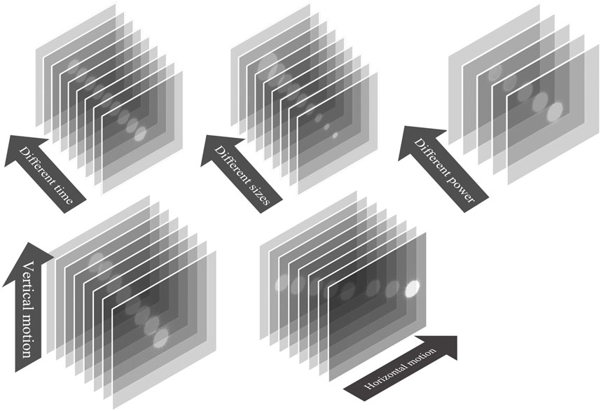
FIGURE 5. Experimental image data.

Repeatability

The localization results of different methods can be seen in Figure 6. Figures 6A–C show the coordinates calculated by each method. The results show that the method based on the Hough transform is the least effective, and it calculates the coordinate positions very randomly. The effect of the circular arc fitting method is unstable, and in Figure 6B, its results have a large deviation in the x-direction. The performance of the gray centroid method is better, and it calculates the coordinate positions more centrally, which is very close to the effect of the method in this paper, we use standard deviation for quantitative analysis and the results are given by Table 1. The standard deviation reflects the degree of dispersion of the data, and when its value is smaller, it means that the data is more concentrated. From Table 1, it is easy to see that the method in this paper performs the best, and the standard deviation of the method in this paper is reduced by 27% on average compared with the traditional gray centroid method.

FIGURE 6

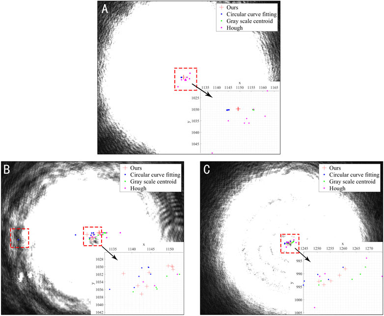
FIGURE 6. Experimental results under the stationary spot position. (A): Different time at the same position; (B): Different sizes at the same position; (C): Different power at the same position.

TABLE 1

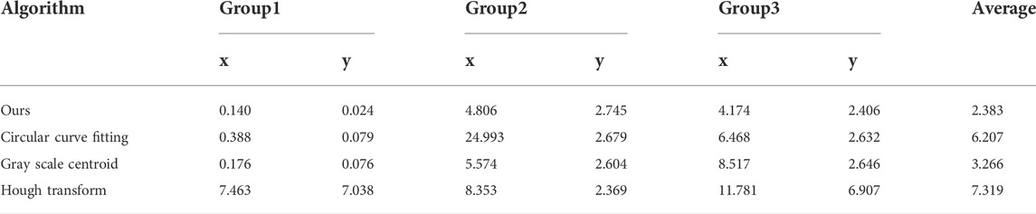
TABLE 1. Standard deviation of coordinate x and coordinate y resulting from different methods.

Linear fitting ability

In this section, the accuracy of different methods is examined by measuring the laser spot centers at different locations. The results of the experiments are shown in Figure 7. We have drawn the visualized paths on the coordinate system. It is easy to notice from Figures 7C,D that the results of Hough transform still look the worst and other method s need to be compared quantitatively.

FIGURE 7

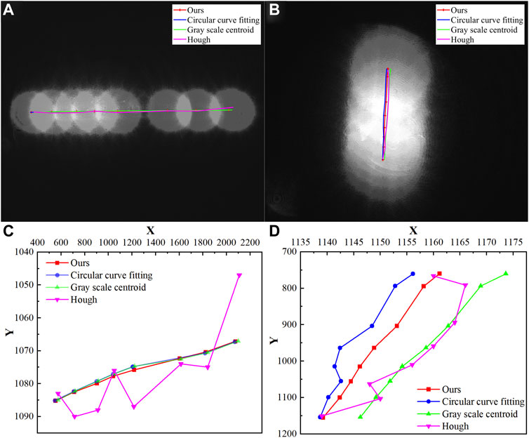
FIGURE 7. Experimental results under the moving spot position. (A): Horizontal direction; (B): Vertical direction; (C): Details in horizontal direction experiment; (D): Details in vertical direction experiment.

Because the laser’s travel path is straight, we perform a linear fit on the results of each algorithm, and the fitting results are shown in Figure 8. When the laser is moved horizontally, the fitting results of different methods are shown in Figures 8A–D. When the laser is moved vertically, the fitting results of different methods are shown in Figures 8E–H. The fitting ability of discrete points can be expressed as Residual Sum of Squares. The smaller the sum of squared residuals, the better the data fit, i.e., the closer the coordinate points are to the true laser spot movement path. For the first row of Figure 8, The laser moves horizontally, the residual at each point is the distance from the point to the vertical of the fitted line. Similarly, in the second row, the residual is the horizontal distance from the point to the fitted line. The detailed calculation results are given in Table 2.

FIGURE 8

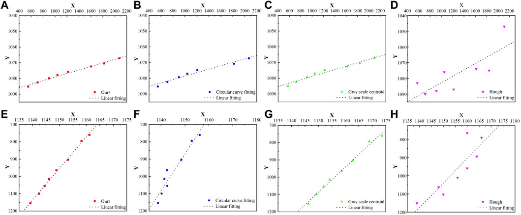
FIGURE 8. Results of fitting straight lines with different methods. (A): Results of our method in horizontal direction; (B): Results of Circular curve fitting method in horizontal direction; (C): Results of Gray scale centroid method in horizontal direction; (D): Results of Hough transform method in horizontal direction; (E): Results of our method in vertical direction; (F): Results of Circular curve fitting method in vertical direction; (G): Results of Gray scale centroid method in vertical direction; (H): Results of Hough transform method in vertical direction;

TABLE 2

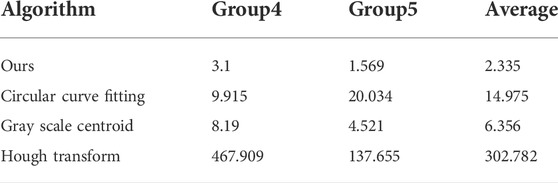
TABLE 2. The Residual sum of squares of the results under different methods.

From Table 2, we can intuitively see that our method fits the best, this means that each coordinate is very close to the trajectory of the laser’s movement. The gray centroid method is the second most effective. The residual sum of squares of the Hough transform is the largest. According to the data in Table 2, Our method reduces the residual sum of squares of the results calculated by the gray scale centroid method by 63.3%, which shows that our method is effective.

Conclusion

This paper focuses on researching the effectiveness of image segmentation based on Chan-Vese model for laser spot center localization. In order to improve the segmentation accuracy, two improvements are made. First, we added image pre-processing to denoise the image using two layers of wavelet decomposition. Second, we improved the initialization coordinates of the level set curve, which drives the evolution of the curve from inside the laser spot. We selected three classical algorithms for comparison, among which the traditional gray centroid method significantly outperformed other algorithms in our dataset. Therefore, we combine our work with the gray scale centroid method and find that it can further improve the accuracy and stability of laser spot positioning, which proves that the image segmentation method based on Chan-Vese model can be applied to laser spot center detection, it provides an idea for method improvement.

Data availability statement

The original contributions presented in the study are included in the article/Supplementary Material, further inquiries can be directed to the corresponding author.

Author contributions

XG proposed the idea and wrote the original manuscript. XG and PM performed the simulation work. DM helped collect the data. PM helped in revising the original manuscript, JS and QJ supervised the research work. HW helped to complete the experiment.

Funding

This work was supported by the National Natural Science Foundation of China Civil Aviation Joint Fund (U1833203) and Graduate Education Innovation Program Fund of Zhengzhou University of Aeronautics (2021CX48).

Conflict of interest

The authors declare that the research was conducted in the absence of any commercial or financial relationships that could be construed as a potential conflict of interest.

Publisher’s note

All claims expressed in this article are solely those of the authors and do not necessarily represent those of their affiliated organizations, or those of the publisher, the editors and the reviewers. Any product that may be evaluated in this article, or claim that may be made by its manufacturer, is not guaranteed or endorsed by the publisher.

References

1. Zhuo H. Laser spot measuring and position method with sub-pixel precision. In: International symposium on photoelectronic detection and imaging 2007: Related technologies and applications, 6625 (2008). p. 66250A. doi:10.1117/12.790760

CrossRef Full Text | Google Scholar

2. Krstinić D, Skelin AK, Milatić I. Laser spot tracking based on modified circular Hough transform and motion pattern analysis. Sensors (2014) 11:20112–33. doi:10.3390/s141120112

PubMed Abstract | CrossRef Full Text | Google Scholar

3. Kong B, Wang Z, Tan Y. Algorithm of laser spot detection based on circle fitting. Infrared Laser Eng (2002) 31:275–9.

Google Scholar

4. Zhang K, Chen H, Li J, Xu J. An improved sub-pixel algorithm for laser spot center determination based on Zernike moments. Proc SPIE - Int Soc Opt Eng (2009) 7382:738244. doi:10.1117/12.836667

CrossRef Full Text | Google Scholar

5. Ballard DH. Generalizing the Hough transform to detect arbitrary shapes. Pattern Recognition (1981) 13:111–22. doi:10.1016/0031-3203(81)90009-1

CrossRef Full Text | Google Scholar

6. Ying J, He Y, Zhou Z. High speed gradient Hough transform algorithm for laser spot location. Proc SPIE - Int Soc Opt Eng (2007) 6625:66250J. doi:10.1117/12.790783

CrossRef Full Text | Google Scholar

7. Moss RH. Optical projection and image processing approach for mine wall monitoring. Opt Eng (2007) 46:013601. doi:10.1117/1.2424914

CrossRef Full Text | Google Scholar

8. Liu Z, Wang Z, Liu S, Shen C. Simulating multiple class urban land-use/cover changes by RBFN-based CA model. Comput Geosci (2011) 28:111–21. doi:10.1016/j.cageo.2010.07.006

CrossRef Full Text | Google Scholar

9. Zhang J. Research on the measurement accuracy of different laser spot center location. Int Conf Photon Opt Eng (2019) 38. doi:10.1117/12.2521709

CrossRef Full Text | Google Scholar

10. Hui L, Zheng S, Cao S, Wang Z. Algorithm of focal spot reconstruction for laser measurement using the schlieren method. Optik (2017) 145:61–5. doi:10.1016/j.ijleo.2017.07.033

CrossRef Full Text | Google Scholar

11. Chen H, Bai Z, Yang X, Ding J, Qi Y, Yan B, et al. Enhanced stimulated Brillouin scattering utilizing Raman conversion in diamond. Appl Phys Lett (2022) 120(18):181103. doi:10.1063/5.0087092

CrossRef Full Text | Google Scholar

12. Bai Z, Williams RJ, Kitzler O, Sarang S, Spence DJ, Wang Y, et al. Diamond Brillouin laser in the visible. APL Photon (2020) 5(3):031301. doi:10.1063/1.5134907

CrossRef Full Text | Google Scholar

13. Wang X, Huang D, Xu H. An efficient local chan–vese model for image segmentation. Pattern Recognition (2010) 43:603–18. doi:10.1016/j.patcog.2009.08.002

CrossRef Full Text | Google Scholar

14. Figueiredo M, Nowak RD. An EM algorithm for wavelet-based image restoration. IEEE Trans Image Process (2003) 12:906–16. doi:10.1109/TIP.2003.814255

PubMed Abstract | CrossRef Full Text | Google Scholar

15. Zhao Z, Bai Z, Jin D, Qi Y, Ding J, Yan B, et al. Narrow laser-linewidth measurement using short delay self-heterodyne interferometry. Opt Express (2022) 30(17):30600–10.

Google Scholar

16. Hun X, Bai Z, Chen B, Wang J, Cui C, Qi Y, et al. Fabry–Pérot based short pulsed laser linewidth measurement with enhanced spectral resolution. Results Phys (2022) 37:105510. doi:10.1016/j.rinp.2022.105510

CrossRef Full Text | Google Scholar

17. Donoho DL, Johnstone IM. Minimax estimation via wavelet shrinkage. Ann Statist (1999) 26:879–921. doi:10.1214/aos/1024691081

CrossRef Full Text | Google Scholar

18. Yang L, Liu G, Shi Z. Research on Suppression Algorithms of the Ringing Effect Caused by Blind Image Restoration. 2015 Fifth International Conference on Instrumentation and Measurement, Computer, Communication and Control (IMCCC) (2015) 1264-1267. doi:10.1109/IMCCC.2015.271

CrossRef Full Text | Google Scholar