Magnetic resonance T1ρ quantification of human brain at 5.0 T: A pilot study

MR quantitative T1ρ mapping has gained increasing attention due to its capability to study low-frequency motional processes and chemical exchange in biological tissues. At ultra-high fields, the chemical exchange and proton diffusion in biological tissues should be more prominent. In this study, for the first time, we aim to test the feasibility of brain T_1ρ mapping at 5.0 T MR scanner and compare the T_1ρ values estimated using 3.0 T and 5.0 T scanners. Preliminary experimental results show that 5.0 T achieves T_1ρ-weighted images with a higher signal-to-noise ratio than those acquired at 3.0T. The SNR benefit at 5.0 T is more obvious in high-resolution imaging. The T_1ρ quantifications at 5.0 T are: Corpus callosum (67.4 ± 1.9 ms), Corona radiate (71.5 ± 1.8 ms), Superior frontal gyrus (67.6 ± 2.5 ms), Putamen (58.9 ± 1.2 ms), Centrum semiovale (84.0 ± 6.3 ms). Statistical analysis results indicate that the T_1ρ values at 5.0 T show no significant difference with those obtained at 3.0 T (all p > 0.05). The interfield agreements in terms of T_1ρ values between 3.0 T and 5.0 T were substantial (all ICCs >0.7). The coefficients of variation for T_1ρ measurements from 3.0 T to 5.0 T were all less than 6.50% (2.28%–6.32%).

Introduction

Magnetic spin-lattice relaxation in the rotation frame (referred to as T_1ρ) is an emerging technique to assess neurodegenerative diseases [1]. Relative to the conventional T₁ and T₂ relaxations, T_1ρ provides a more specific probe of motional interactions related to the exchanges that are on the time scale of the reciprocal of the spin lock field strength. It is sensitive to the local tissue microenvironment and microstructure, such as the pH and glucose levels. Previous studies have demonstrated that proton exchange between bulk water and labile protons of protein or metabolites is an important contributor to the low-frequency T_1ρ dispersion in biological tissue [2–5]. Therefore, T_1ρ has been considered a potential biomarker for the evaluation and early diagnoses of degenerative neurologic diseases, such as multiple sclerosis [6–8], Alzheimer’s disease [9–11], Parkinson disease [12–14], and stroke [15,16].

T_1ρ quantification is performed by fitting a series of T_1ρ-weighted images acquired at varying spin-lock durations (TSL), which can be obtained using most magnetic resonance imaging (MRI) sequences by including a spin-lock preparation pulse at the beginning of the sequence. The T_1ρ imaging technique is sensitive to the B₀ and B₁ field inhomogeneities and usually has a high specific absorption rate (SAR) due to the spin-lock pulse. Therefore, most T_1ρ studies were performed at typically 1.5 T or 3.0 T fields, and human studies of T_1ρ quantification at ultra-high fields were rarely reported [17–19]. At the ultra-high field, chemical exchanges between sites of different chemical shifts increase rapidly with field strength and may significantly contribute to the rotating frame relaxations [20]. T_1ρ relaxation occurs in response to the chemical exchange between the groups of spins, which depends on chemical shift, temperature, exchange rate of the exchanging spins, etc. [21]. It is hence well suited for probing the metabolic information at higher magnetic field strengths [18,22]. Furthermore, high-resolution T_1ρ quantification can be achieved using an ultra-high field MR scanner with a high signal-to-noise ratio (SNR) and affords improved morphological detail compared to imaging at lower-field strength [7] in an effort to improve visualization of brain lesions.

Last year, the first 5.0 T ultra-high field whole-body MR system (Jupiter, United Imaging Healthcare, Shanghai, China) was delivered. Compared with the 7.0 T ultra-high field system, the magnetic field strength of 5.0 T system has fewer SAR and field inhomogeneity. These advantages may bring benefits to brain T_1ρ quantification. We implemented a three-dimensional (3D) T_1ρ mapping sequence in this system, using a spin-lock T_1ρ preparation pulse followed by a gradient recalled echo (GRE) readout, and applied it to imaging the brain of healthy volunteers. In this study, we will report the T_1ρ quantification of the human brain at 5.0 T for the first time. Also, the SNR and spatial resolution gains of brain T_1ρ images obtained from 5.0 T are demonstrated, and corresponding T_1ρ values obtained from 5.0 T are compared with those obtained from 3.0 T.

Materials and methods

Subjects

The experiments were approved by the local Institutional Review Board (IRB). Twelve healthy volunteers (10 males, age: 30 ± 5 years; 2 females, age: 28 ± 4 years) were recruited in this study, and informed consent was obtained from each volunteer before the scan. All subjects participated in this study were scanned at a 5.0 T scanner (Jupiter, United Imaging Healthcare, Shanghai, China) and a 3.0 T scanner (uMR 890, United Imaging Healthcare, Shanghai, China). A modified T_1ρ preparation pulse sequence based on a previously reported sequence was used [17].

Imaging sequence

The imaging sequence is depicted in Figure 1. The pulse sequence starts with a 90-degree RF pulse followed by crusher gradients to reset the net magnetization, which assures the signal is constant at the beginning of T_1ρ preparation pulse [23]. The following recovery time (T_rec) allows the recovery of the magnetization before the T_1ρ preparation pulse and the acquisition. An adiabatically prepared constant-amplitude on-resonant spin-lock preparation pulse is used for T_1ρ preparation [17], which is robust to B₀ and B₁ inhomogeneities. It consists of a rectangular locking pulse sandwiched by an adiabatic half passage (AHP) pulse and a reverse adiabatic half passage (RAHP) pulse[24,25]. The adjusted hyperbolic secant pulses are used as the AHP and RAHP. After the T_1ρ preparation pulse, the residual transverse magnetization is destroyed by a gradient crusher. Then a 3D segmented radiofrequency gradient echo (GRE) sequence is employed for signal acquisition using the centric phase encoding order [26,27].

FIGURE 1

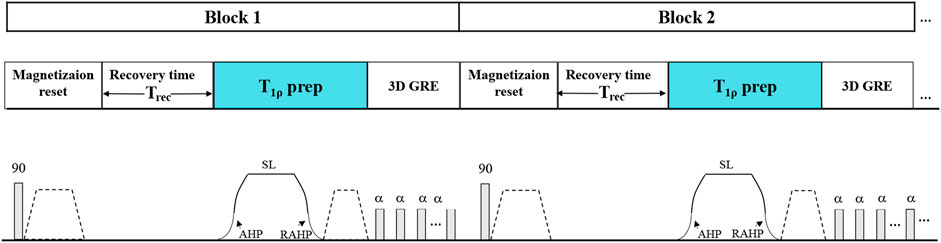
FIGURE 1. The timing diagram of the 3D T_1ρ imaging sequence. The T_1ρ preparation pulse was accomplished using an adiabatically prepared constant-amplitude on-resonant spin-lock approach to compensate for the B₀ and B₁ inhomogeneities at 5.0 T.

The 3D T_1ρ imaging was performed with spin-lock pulse amplitude B_1sl = 500 Hz and TSL = 0, 25, 45, and 65 ms at the 5.0 T and 3.0 T scanners. The 5.0 T MR scanner used a local quadrature birdcage transmit and 48-channel receiver head coil [28]. At the 3.0 T MR scanner, a commercial 32-channel receiver head coil (Rx: 32 channel) was used for T_1ρ imaging. Three datasets were acquired for each subject at each scanner. Two datasets were acquired with a regular resolution of 1 × 1 × 3 mm³ in the sagittal and coronal orientations, respectively. Another was acquired with a high resolution of 0.65 × 0.65 × 2.5 mm³ in the transverse orientation. The imaging parameters are depicted in Table 1.

TABLE 1

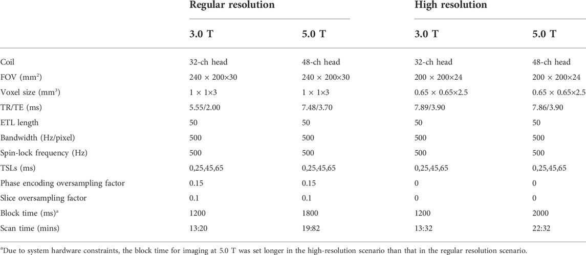
TABLE 1. Imaging parameters for T_1ρ quantification of the human brain at 5.0 T and 3.0 T

Data analysis

All T_1ρ quantification and analysis were performed in Matlab R2017b (MathWorks, Natick, MA, United States). The T_1ρ maps were estimated using the exponential model [29,30] by fitting the T_1ρ-weighted images with different TSLs pixel-by-pixel:

$M_n=M_0{\mathit{exp}\left(-{TSL}_n/T_{1\rho }\right)}_{n=\mathrm{1,2},\dots ,N}(1)$

where $M_n$ is the image intensity obtained at varying TSLs, M₀ is the baseline image intensity without applying the spin-lock pulse. T_1ρ map was estimated using the nonlinear least-squares fitting method with the Levenberg–Marquardt algorithm [31] from the T_1ρ-weighted images.

Five regions of interest (ROIs) were manually drawn on the images of each volunteer by two independent readers (with 5-year experience in neural imaging), including Corpus callosum, Corona radiate, Superior frontal gyrus, Putamen, and Centrum semiovale. The average T_1ρ value in each ROI was calculated, and the correlation of the T_1ρ measurements between 3.0 T and 5.0 T was analyzed.

The SNRs of T_1ρ-weighted images obtained from 5.0 T were also calculated and compared with those obtained from 3.0 T. The SNR was defined as the ratio between the mean value of the imaging regions and the standard deviation (SD) of the background noise [32]. To reduce the subject bias, four ROIs were drawn on each slice to calculate the noise SD and the SNR. Final SNR (denoted as SNR_T1ρ-w) was calculated as the average of these four SNRs. Mean values and SDs of SNR_T1ρ-w were computed for all the volunteers in each orientation.

Statistical analysis

The difference and consistency of T_1ρ values measured at 3.0 T and 5.0 T were statistically compared using the Mann-Whitney U test. The intraclass correlation coefficients (ICCs) and Bland–Altman analysis were used to evaluate the interfield agreements and to determine whether there were significant differences in terms of T_1ρ values between 3.0 T and 5.0 T. The interfield agreement was considered to be poor for ICCs = 0.0–0.2, fair for ICCs = 0.2–0.4, moderate for ICCs = 0.4–0.6, substantial for ICCs = 0.6–0.8, and excellent for ICCs = 0.8–1.0. p < 0.05 was considered statistically significant. The coefficient of variation (CV = std_T1ρ/mean_T1ρ) was used to assess the variability and reliability of T_1ρ values measured at 3.0 T and 5.0 T. CVs <15%, between 15% and 35% and >35% were considered to be small, moderate, and large variability. Statistical analyses were performed using SPSS 25.0 (IBM, Armonk, NY) and MedCalc 20.0.22 (MedCalc Software, Mariakerke, Belgium).

Results

Imaging with regular resolution

Figure 2 shows the representative T_1ρ-weighted images at TSL = 0 and 65 ms of one subject with the regular resolution at 3.0 T and 5.0 T in the sagittal and coronal orientations, respectively. The noticeable difference between the image contrasts of 3.0 T and 5.0 T might be due to the change of relaxation time with the field strength. In addition, visible noise can be observed in the T_1ρ-weighted images at 3.0 T, especially at TSL = 65 ms, since the signal attenuates with the increase of TSL. The corresponding T_1ρ maps of the above T_1ρ-weighted images are shown in Figure 3. These maps show extensive spatial similarities present between 3.0 T and 5.0 T T_1ρ values for the same volunteers, except that the T_1ρ maps at 3.0 T are a little noisier than those at 5.0 T.

FIGURE 2

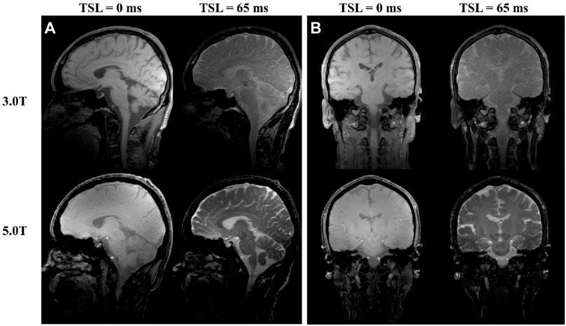
FIGURE 2. The T_1ρ-weighted images with different TSLs collected at 3.0 T and 5.0 T.

FIGURE 3

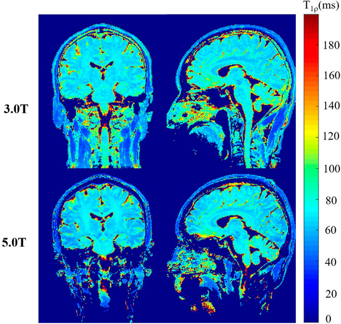
FIGURE 3. The T_1ρ maps obtained at 3.0 T and 5.0 T.

Imaging with high resolution

Figure 4 shows T_1ρ-weighted images of different TSLs and the corresponding T_1ρ maps in the high-resolution scenario for an axial slice from two subjects acquired at 3.0 T and 5.0 T. Similar conclusions to the regular scenario can be obtained. Furthermore, the SNRs of T_1ρ-weighted images obtained at 3.0 T drop significantly due to the increased resolution. As the signal decays exponentially along the TSL direction, some image details are almost drowned out by noise, especially at longer TSLs. Correspondingly, the T_1ρ maps also seem noisy. However, the T_1ρ-weighted images obtained at 5.0 T still show good image detail with reasonable SNRs, and the image quality of T_1ρ maps is also improved.

FIGURE 4

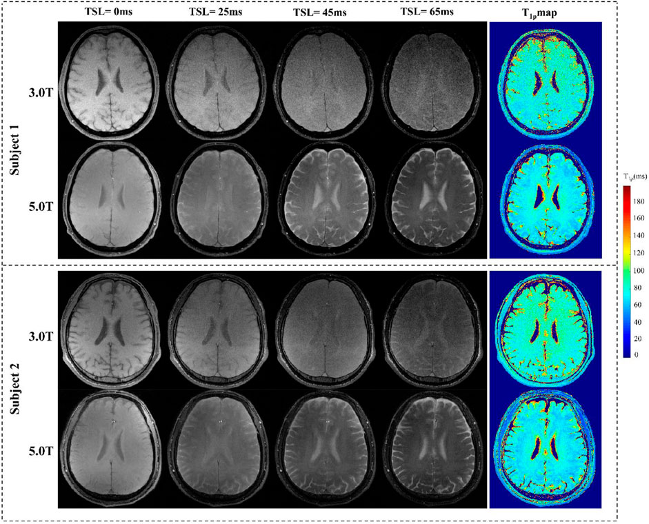
FIGURE 4. T_1ρ-maps estimated from datasets collected at 3.0 T and 5.0 T.

T_1ρ measurements and signal-to-noise ratio analysis

The T_1ρ values in the tissue compartments of the selected ROIs at 5.0 T and 3.0 T are shown in Table 2. There was no significant difference between the T_1ρ values obtained at 5.0 T and 3.0 T (all p > 0.05). The ICCs for evaluating the interfield agreements are also shown in Table 2. LCI and UCI are the abbreviations of the lower and upper bounds of the 95% confidence interval. The ICCs of T_1ρ values in all tissue compartments between 3.0 T and 5.0 T were as follows: ICC_{Corpus callosum} = 0.730 [95% confidence interval (CI): 0.499–0.865]; ICC_{Corona radiate} = 0.725 (95% CI:−0.466–0.869); ICC_{Superior frontal gyrus} = 0.788 (95% CI: 0.576–0.901); ICC_Putamen = 0.788 (95% CI: 0.461–0.882) and ICC_{Centrum semiovale} = 0.768 (95% CI: 0.542–0.890). All ICCs between the 3.0 T and 5.0 T were >0.7, indicating substantial agreements.

TABLE 2

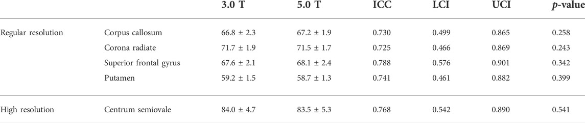
TABLE 2. Average T_1ρ values of selected ROIs and the corresponding p-values at 3.0 T and 5.0 T

The SNR of the T_1ρ-weighted images obtained at 5.0 T and 3.0 T are shown in Table 3. As expected, the image SNR at 5.0 T was higher than that at 3.0 T, and significant differences were seen between the SNRs obtained at 5.0 T and 3.0 T, with p < 0.05 for all imaging scenarios. On average, with the regular resolution, the SNR of the T_1ρ-weighted images obtained at 5.0 T was 15.67% higher than that at 3.0 T, and this value increased to 46.6% in the high-resolution scenario.

TABLE 3

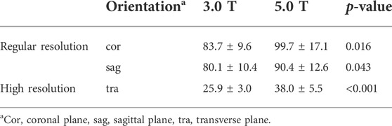
TABLE 3. The average SNR of the T_1ρ-weighted images obtained at 3.0 T and 5.0 T

The coefficient of variation between the 3.0 T and 5.0 T T_1ρ values for five selected ROIs are shown in Table 4. For 3.0 T, the CVs of T_1ρ values for Corpus callosum, Corona radiate, Superior frontal gyrus, Putamen, Centrum semiovale were 3.42%, 2.70%, 3.14%, 2.58%, respectively, and the CVs of T_1ρ values from 5.0 T were 2.79%, 2.36%, 3.48%, 2.28%. Based on the above results, the variability of T_1ρ values at different field strengths for five selected ROIs was determined as small (CV < 15.0%).

TABLE 4

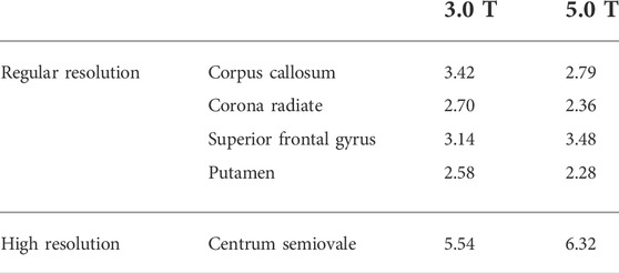
TABLE 4. The Coefficient of Variation (%) of T_1ρ values for selected ROIs at 3.0 T and 5.0 T

The Bland-Altman plots of the mean interfield differences of T_1ρ values (T_1ρ difference = T_1ρ,3.0 T- T_1ρ,5.0 T) for the five tissue compartments in the aforementioned ROIs are shown in Figure 5, and the mean interfield differences of T_1ρ values are as follows: T_1ρ difference of Corpus callosum: mean ±1.96SD: −3.4–2.5 ms, bias: −0.4361 ms, 95% CI: −1.0214, 0.1493; T_1ρ difference of Corona radiate: mean ±1.96SD: −2.6–2.7 ms, bias: 0.0616 ms, 95% CI: −0.5006, 0.6238; T_1ρ difference of Superior frontal gyrus: mean ±1.96SD: −3.3–2.3 ms, bias: −0.4864 ms, 95% CI: −1.0732, 0.1004; T_1ρ difference of Putamen: mean ±1.96SD: −1.4–2.4 ms, bias: 0.4784 ms, 95% CI: −0.0818, 0.8750; T_1ρ difference of Centrum semiovale: mean ± SD: −4.7–6.0 ms, bias:0.6504 ms, 95% CI: −0.4798, 1.7806.

FIGURE 5

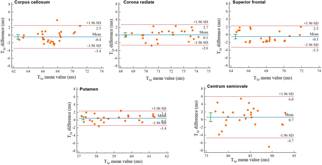
FIGURE 5. Bland–Altman plots of T_1ρ difference values at 5.0 T relative to the T_1ρ values at 3.0 T in the Corpus callosum, Corona radiate, Superior frontal gyrus, Putamen, and Centrum semiovale. The solid and dashed lines in the Bland-Altman plots represent the bias and ±1.96 × standard deviation, respectively.

Discussion

In this study, we demonstrated the feasibility of brain T_1ρ quantification at 5.0 T and compared the T_1ρ values to 3.0 T in healthy volunteers. T_1ρ mapping at higher field strengths benefits from increased SNR and chemical exchange, resulting in its increased sensitivity to exchange effects, such as changes in macromolecule concentrations. In previous studies, T_1ρ mapping at 7.0 T has shown great potential in studying the loss of proteoglycan and improving differentiation between knees with cartilage lesions and controls, and it is also promising for glucose metabolism studies in detecting intracerebral regions of increased glucose concentration [18,33]. However, SAR limits should be carefully taken into account since the spin lock pulse requires a large amount of RF energy. Relative to 7.0 T, T_1ρ mapping at 5.0 T has met less resistance due to lower SAR of spin lock pulse. In addition, the use of the adiabatically prepared spin-lock preparation pulse can compensate for the B₀ and B₁ inhomogeneities at 5.0 T, which are also lower than those at 7.0 T. Thus, we can obtain reliable T_1ρ maps of the brain. To our knowledge, this is the first depiction of brain T_1ρ mapping at 5.0 T.

High-resolution anatomical images are desirable for better clinical diagnostic details and clearer visualization of morphological abnormalities. Additionally, it hold great potential for investigation and characterization of various pathological processes. For example, demyelination and axonal loss across various brain regions are prevalent at very early stages of multiple sclerosis [7]. These high-resolution images can improve gray matter and white matter differentiation, in an effort to classify the location of lesions in relation to the cortical/subcortical boundary [34]. While in the case of lower resolution, effects of partial of skull with this free fluid would be increased and could confound interpretation of results.

Our experimental results showed that the image SNRs of T_1ρ-weighted images were significantly improved at 5.0 T, and the improvement became more obvious in the high-resolution scenario. This result was in good concordance with previous studies [34–36]. Since SNR is linearly proportional to the magnetic field strength, ultra-high field MRI affords higher spatial resolution, allowing for the visualization of small anatomic structures not previously appreciated at lower magnetic field strengths. As shown in Table 2, the T_1ρ values of the brain obtained at 5.0 T are not significantly different from those obtained at 3.0 T. This indicates that the T_1ρ values obtained at 5.0 T can be utilized for brain investigation, which is valuable for longitudinal investigation and comparison. Although increasing the number of averages will increase the SNR, it also enables exponential increase in the scan time. However, it may be also hard to use a different number of averages to make the scanning time of 3.0 T equal to 5.0 T. We calculated the SNR per unit of time for images at 5.0 T and 3.0 T respectively by dividing the SNR by the square root of the scanning time. Since the TE of imaging at 5.0 T is different from that at 3.0 T in the regular resolution scenario, due to different duration, gradient ramp and gradient amplitude of the readout gradient, we calculated the SNR per unit of time for images in the high resolution scenario for fair comparison. According to the SNR results in Table 3, the SNR per unit of time for images collected at 5.0 T is also higher than that at 3.0 T, with the value of 8.01 (s⁻¹) at 5.0 T, and 7.05 (s⁻¹) at 3.0 T, respectively.

In this study, since the imaging sequence contains the long-duration T_1ρ-preparation pulse, the energy deposited into tissues needs to be addressed, especially for the ultra-high field MR systems. According to previous studies [37–39], the SAR for a single pulse used in the sequence can be estimated as:

${\mathrm{S}\mathrm{A}\mathrm{R}}_{\tau /\alpha }={\mathrm{f}\left(\frac{3\mathrm{m}\mathrm{s}}{\mathrm{\tau }}\right)}^2{\left(\alpha /90°\right)}^2{SAR}_{3ms/90°}(2)$

where $\tau$ is the duration (in ms), $\alpha$ is the flip angle, f is a pulse shape factor determined by the type of pulse used, which equals 1 for a hard pulse, or equals 0.67 for a Gaussian pulse, or equals 2 for a sinc pulse. ${\mathrm{S}\mathrm{A}\mathrm{R}}_{3ms/90°}$ denotes the SAR for a 90°hard pulse with a duration of 3 ms. ${SAR}_{3ms/90°}$at 3.0 T for the head model was estimated between 0.242 W/kg (1.5 T) and 2.16 W/kg (4.1 T), and ${SAR}_{3ms/90°}$at 5.0T for the head model was slightly larger than 3.3 W/kg (4.7 T). The average SAR delivered for the pulse sequence is the sum of energy absorbed by each RF pulse divided by the total time to acquire the image:

$\mathrm{S}\mathrm{A}\mathrm{R}=\frac{{\displaystyle \sum }_{n=1}^N{\mathrm{S}\mathrm{A}\mathrm{R}}_{{\tau }_n/{\alpha }_n}\times {\tau }_n}{T_{total}}(3)$

where ${\mathrm{S}\mathrm{A}\mathrm{R}}_{\tau /\alpha }$ is calculated using Eq. 2, SAR denotes the average delivered SAR over the total time period $T_{total}$, N denotes the number of RF pulses. The Food and Drug Administration (FDA) mandated maximum SAR level that equals 3W/kg of the head during the extremities averaged over 10 min. In this study, the average SAR delivered to the brain with TSL = 65 ms approximately 2.68 W/kg at 5.0T and between 0.22 W/kg and 1.98 W/kg at 3.0 T.

In this study, TSL times were chosen empirically based on hardware limitations. The allowed maximum RF duration depends on the RF hardware of the system. In previous studies [6,39–41], the T_1ρ-weighted images were produced by using an RF pulse cluster (e.g. 90°_+x–SL_+y –180°_+y–SL_-y –90°_+x), it is easy to set the TSL to 100 ms due to using the composite SL pulses. In the UIH MR scanner, the deadtime between two pulses is 200us, which is much larger than other commercial MR scanners. The dephasing during the deadtime will affect the image quality of T_1ρ-weighted images and may result in inaccurate T_1ρ mapping. To resolve this problem and to compensate for the B₀ and B₁ inhomogeneity, we used a single pulse to improve the robustness of T_1ρ imaging. The maximum duration allowed of a single pulse is around 80 ms, both on the 3.0 T and 5.0T UIH MR scanners. Got rid of the time for AHP and RAHP, the maximum TSL used was 65 ms in our study. In our future work, optimized T_1ρ preparation pulses with longer TSL and insensitive to B₀ and B₁ field inhomogeneity will be studied.

Although several studies of knee cartilage showed that 7.0 T T_1ρ values were slightly lower than 3.0 T T_1ρ values [33,42], the dependence between the T_1ρ value and the B₀ field strength is not very clear for brain tissues. As is shown in Table 5, we listed the T_1ρ values of white matter and gray matter at different field strengths reported in previous studies. The T_1ρ values of white matter and gray matter at 3.0 T in our study are consistent with previous studies (T_1ρ of the white matter: 76.07 ms, T_1ρ of gray matter: 80.1 ms). And T_1ρ measurements at 5.0 T showed no significant difference with that at 3.0 T, with the current imaging protocols. Theoretically, the chemical exchange and diffusion contribution to the T_1ρ increases with the magnetic field, the field-dependent trend of the T_1ρ relaxation times is less pronounced than that of T₁ in this study, which is similar to the T₂ relaxation times [43].

TABLE 5

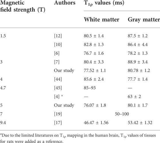
TABLE 5. T_1ρ values for white matter and gray matter at different magnetic field strengths.

There were several limitations in this study. First, the scan time of T_1ρ quantification is relatively long due to the requirement of acquiring multiple images with different TSLs. There might be a subject’s motion during acquisition. Fast MRI techniques such as compressed sensing and deep learning can shorten the scan time to a clinically acceptable range but have not yet been integrated into the 5.0 T scanner. Second, the slice thickness is up to 3 mm in this study, which may cause some small lesions to be missed, or inaccurate characterization of lesions due to partial volume effects in clinical applications. Future technical improvement will focus on shortening the scan time for higher-resolution imaging by using the abovementioned fast MRI techniques. Third, all of the subjects were healthy volunteers, and no patient was included in this study. Since the T_1ρ values of patients may be different from that of healthy volunteers, efforts should be made to further evaluate the T_1ρ quantification of brain lesions at 5.0 T for patients with neurologic diseases and investigate the ability of T_1ρ mapping to determine differences between normal and patients.

Conclusion

This study confirmed the feasibility of brain T_1ρ quantification at 5.0 T. There was no significant difference between the brain T_1ρ values obtained at 3.0 T and 5.0 T. The SNR of T_1ρ-weighted images was significantly improved at 5.0 T relative to 3.0 T, which is a benefit for high-resolution imaging and dispersion-related studies. The T_1ρ quantification at 5.0 T may be reliable for clinical investigations.

Data availability statement

The original contributions presented in the study are included in the article/supplementary material, further inquiries can be directed to the corresponding authors.

Ethics statement

The studies involving human participants were reviewed and approved by the Ethics Committee at the Shenzhen Institute of Advanced Technology, Chinese Academy of Sciences (Ethics Committee approval number: YSB-2022-Y02088). The patients/participants provided their written informed consent to participate in this study.

Author contributions

YL: conceptualization, methodology, software, writing—original draft. WW: Formal analysis, data curation, visualization, writing—original draft. YZ: investigation, formal analysis, validation. HW: supervision. HZ: supervision. DL: supervision, writing—review and editing, funding acquisition. YZ: writing—review and editing, supervision, project administration, funding acquisition.

Funding

This study is supported by the National Key R&D Program of China no. 2020YFA0712200, National Natural Science Foundation of China under grant no. 62201561, 81971611, 62125111, 81901736, and U1805261, the Guangdong Basic and Applied Basic Research Foundation under grant no. 2021A1515110540, the Key Technology and Equipment R&D Program of Major Science and Technology Infrastructure of Shenzhen under grant no. 202100102, 202100104, Shenzhen Science and Technology Program under grant no. RCYX20210609104444089.

Conflict of interest

The authors declare that the research was conducted in the absence of any commercial or financial relationships that could be construed as a potential conflict of interest.

Publisher’s note

All claims expressed in this article are solely those of the authors and do not necessarily represent those of their affiliated organizations, or those of the publisher, the editors and the reviewers. Any product that may be evaluated in this article, or claim that may be made by its manufacturer, is not guaranteed or endorsed by the publisher.

References

1. Wang YX, Zhang Q, Li X, Chen W, Ahuja A, Yuan J. T1ρ magnetic resonance: Basic physics principles and applications in knee and intervertebral disc imaging. Quant Imaging Med Surg (2015) 5:858–85. doi:10.3978/j.issn.2223-4292.2015.12.06

PubMed Abstract | CrossRef Full Text | Google Scholar

2. Jin T, Kim SG. Characterization of non-hemodynamic functional signal measured by spin-lock fMRI. Neuroimage (2013) 78:385–95. doi:10.1016/j.neuroimage.2013.04.045

PubMed Abstract | CrossRef Full Text | Google Scholar

3. Kettunen MI, Grohn OH, Silvennoinen MJ, Penttonen M, Kauppinen RA. Effects of intracellular pH, blood, and tissue oxygen tension on T1ρ relaxation in rat brain. Magn Reson Med (2002) 48:470–7. doi:10.1002/mrm.10233

PubMed Abstract | CrossRef Full Text | Google Scholar

4. Kettunen MI, Sierra A, Narvainen MJ, Valonen PK, Yla-Herttuala S, Kauppinen RA, et al. Low spin-lock field T1 relaxation in the rotating frame as a sensitive MR imaging marker for gene therapy treatment response in rat Glioma¹. Radiology (2007) 243:796–803. doi:10.1148/radiol.2433052077

PubMed Abstract | CrossRef Full Text | Google Scholar

5. Magnotta VA, Heo HY, Dlouhy BJ, Dahdaleh NS, Follmer RL, Thedens DR, et al. Detecting activity-evoked pH changes in human brain. Proc Natl Acad Sci U S A (2012) 109:8270–3. doi:10.1073/pnas.1205902109

PubMed Abstract | CrossRef Full Text | Google Scholar

6. Gonyea JV, Watts R, Applebee A, Andrews T, Hipko S, Nickerson JP, et al. In vivo quantitative whole-brain T1ρ MRI of multiple sclerosis. J Magn Reson Imaging (2015) 42:1623–30. doi:10.1002/jmri.24954

PubMed Abstract | CrossRef Full Text | Google Scholar

7. Ma S, Wang N, Fan Z, Kaisey M, Sicotte NL, Christodoulou AG, et al. Three-dimensional whole-brain simultaneous T1, T2, and T1ρ quantification using MR Multitasking: Method and initial clinical experience in tissue characterization of multiple sclerosis. Magn Reson Med (2021) 85:1938–52. doi:10.1002/mrm.28553

PubMed Abstract | CrossRef Full Text | Google Scholar

8. Mangia S, Carpenter AF, Tyan AE, Eberly LE, Garwood M, Michaeli S. Magnetization transfer and adiabatic T1ρ MRI reveal abnormalities in normal-appearing white matter of subjects with multiple sclerosis. Mult Scler (2014) 20:1066–73. doi:10.1177/1352458513515084

PubMed Abstract | CrossRef Full Text | Google Scholar

9. Boles Ponto LL, Magnotta VA, Menda Y, Moser DJ, Oleson JJ, Harlynn EL, et al. Comparison of T₁Rho MRI, glucose metabolism, and amyloid burden across the cognitive spectrum: A pilot study. J Neuropsychiatry Clin Neurosci (2020) 32:352–61. doi:10.1176/appi.neuropsych.19100221

PubMed Abstract | CrossRef Full Text | Google Scholar

10. Borthakur A, Sochor M, Davatzikos C, Trojanowski JQ, Clark CM. T1ρ MRI of Alzheimer's disease. Neuroimage (2008) 41:1199–205. doi:10.1016/j.neuroimage.2008.03.030

PubMed Abstract | CrossRef Full Text | Google Scholar

11. Haris M, Yadav SK, Rizwan A, Singh A, Cai K, Kaura D, et al. T1rho MRI and CSF biomarkers in diagnosis of Alzheimer's disease. NeuroImage: Clin (2015) 7:598–604. doi:10.1016/j.nicl.2015.02.016

PubMed Abstract | CrossRef Full Text | Google Scholar

12. Haris M, Singh A, Cai KJ, Davatzikos C, Trojanowski JQ, Melhem ER, et al. T1rho (T1ρ) MR imaging in Alzheimer’ disease and Parkinson’s disease with and without dementia. J Neurol (2011) 258:380–5. doi:10.1007/s00415-010-5762-6

PubMed Abstract | CrossRef Full Text | Google Scholar

13. Mangia S, Svatkova A, Mascali D, Nissi MJ, Burton PC, Bednarik P, et al. Multi-modal brain MRI in subjects with PD and iRBD. Front Neurosci (2017) 11:709. doi:10.3389/fnins.2017.00709

PubMed Abstract | CrossRef Full Text | Google Scholar

14. Nestrasil I, Michaeli S, Liimatainen T, Rydeen CE, Kotz CM, Nixon JP, et al. T1ρ and T2ρMRI in the evaluation of Parkinson's disease. J Neurol (2010) 257:964–8. doi:10.1007/s00415-009-5446-2

PubMed Abstract | CrossRef Full Text | Google Scholar

15. Jokivarsi KT, Hiltunen Y, Grohn H, Tuunanen P, Grohn OHJ, Kauppinen RA. Estimation of the onset time of cerebral ischemia using T1ρand T2 MRI in rats. Stroke (2010) 41:2335–40. doi:10.1161/strokeaha.110.587394

PubMed Abstract | CrossRef Full Text | Google Scholar

16. Tan YF, Xu J, Chen RY, Chen B, Xu J, Ren DK, et al. Use of T1 relaxation time in rotating frame (T1ρ) and apparent diffusion coefficient to estimate cerebral stroke evolution. J Magn Reson Imaging (2018) 48:1247–54. doi:10.1002/jmri.25971

PubMed Abstract | CrossRef Full Text | Google Scholar

17. Herz K, Gandhi C, Schuppert M, Deshmane A, Scheffler K, Zaiss M. CEST imaging at 9.4 T using adjusted adiabatic spin-lock pulses for on- and off-resonant T1ρ-dominated Z-spectrum acquisition. Magn Reson Med (2019) 81:275–90. doi:10.1002/mrm.27380

PubMed Abstract | CrossRef Full Text | Google Scholar

18. Paech D, Schuenke P, Koehler C, Windschuh J, Mundiyanapurath S, Bickelhaupt S, et al. T1ρ-weighted dynamic glucose-enhanced MR imaging in the human brain. Radiology (2017) 285:914–22. doi:10.1148/radiol.2017162351

PubMed Abstract | CrossRef Full Text | Google Scholar

19. Schuenke P, Koehler C, Korzowski A, Windschuh J, Bachert P, Ladd ME, et al. Adiabatically prepared spin-lock approach for T1ρ-based dynamic glucose enhanced MRI at ultrahigh fields. Magn Reson Med (2017) 78:215–25. doi:10.1002/mrm.26370

PubMed Abstract | CrossRef Full Text | Google Scholar

20. Spear JT, Gore JC. New insights into rotating frame relaxation at high field. NMR Biomed (2016) 29:1258–73. doi:10.1002/nbm.3490

PubMed Abstract | CrossRef Full Text | Google Scholar

21. Gilani IA, Sepponen R. Quantitative rotating frame relaxometry methods in MRI. NMR Biomed (2016) 29:841–61. doi:10.1002/nbm.3518

PubMed Abstract | CrossRef Full Text | Google Scholar

22. Jin T, Iordanova B, Hitchens TK, Modo M, Wang P, Mehrens H, et al. Chemical exchange-sensitive spin-lock (CESL) MRI of glucose and analogs in brain tumors. Magn Reson Med (2018) 80:488–95. doi:10.1002/mrm.27183

PubMed Abstract | CrossRef Full Text | Google Scholar

23. Chen WT, Chan Q, Wang YXJ. Breath-hold black blood quantitative T1rho imaging of liver using single shot fast spin echo acquisition. Quant Imaging Med Surg (2016) 6:168–77. doi:10.21037/qims.2016.04.05

PubMed Abstract | CrossRef Full Text | Google Scholar

24. Chen W. Artifacts correction for T1rho imaging with constant amplitude spin-lock. J Magn Reson (2017) 274:13–23. doi:10.1016/j.jmr.2016.11.002

PubMed Abstract | CrossRef Full Text | Google Scholar

25. Garwood M, DelaBarre L. The return of the frequency sweep: Designing adiabatic pulses for contemporary NMR. J Magn Reson (2001) 153:155–77. doi:10.1006/jmre.2001.2340

PubMed Abstract | CrossRef Full Text | Google Scholar

26. Johnson CP, Thedens DR, Kruger SJ, Magnotta VA. Three-Dimensional GRE T1ρ mapping of the brain using tailored variable flip-angle scheduling. Magn Reson Med (2020) 84:1235–49. doi:10.1002/mrm.28198

PubMed Abstract | CrossRef Full Text | Google Scholar

27. Li X, Han ET, Busse RF, Majumdar S. In vivo T1ρ mapping in cartilage using 3D magnetization-prepared angle-modulated partitioned k-space spoiled gradient echo snapshots (3D MAPSS). Magn Reson Med (2008) 59:298–307. doi:10.1002/mrm.21414

PubMed Abstract | CrossRef Full Text | Google Scholar

28. Wei Z, Chen Q, He Q, Zhang X, Liu X, zheng H, Li Y. A quadrature birdcage/48-channel receiver coil assembly for human brain imaging at 5T. In: 2022 Joint Annual Meeting ISMRM-ESMRMB & ISMRT 31st Annual Meeting; London (2022).

Google Scholar

29. Zhu Y, Liu Y, Ying L, Peng X, Wang YJ, Yuan J, et al. SCOPE: Signal compensation for low-rank plus sparse matrix decomposition for fast parameter mapping. Phys Med Biol (2018) 63:185009. doi:10.1088/1361-6560/aadb09

PubMed Abstract | CrossRef Full Text | Google Scholar

30. Zhu Y, Liu Y, Ying L, Qiu Z, Liu Q, Jia S, et al. A 4-minute solution for submillimeter whole-brain T1ρ quantification. Magn Reson Med (2021) 85:3299–307. doi:10.1002/mrm.28656

PubMed Abstract | CrossRef Full Text | Google Scholar

31. Moré JJ. The levenberg-marquardt algorithm: Implementation and theory. Numer Anal (1978) 105–16. doi:10.1007/BFb0067700

CrossRef Full Text | Google Scholar

32. Firbank MJ, Coulthard A, Harrison RM, Williams ED. A comparison of two methods for measuring the signal to noise ratio on MR images. Phys Med Biol (1999) 44:N261–4. doi:10.1088/0031-9155/44/12/403

PubMed Abstract | CrossRef Full Text | Google Scholar

33. Wyatt C, Guha A, Venkatachari A, Li XJ, Krug R, Kelley DE, et al. Improved differentiation between knees with cartilage lesions and controls using 7T relaxation time mapping. J Orthopaedic Translation (2015) 3:197–204. doi:10.1016/j.jot.2015.05.003

PubMed Abstract | CrossRef Full Text | Google Scholar

34. Springer E, Dymerska B, Cardoso PL, Robinson SD, Weisstanner C, Wiest R, et al. Comparison of routine brain imaging at 3 T and 7 T. Invest Radiol (2016) 51:469–82. doi:10.1097/rli.0000000000000256

PubMed Abstract | CrossRef Full Text | Google Scholar

35. Metcalf M, Xu D, Okuda DT, Carvajal L, Srinivasan R, Kelley DA, et al. High-resolution phased-array MRI of the human brain at 7 tesla: Initial experience in multiple sclerosis patients. J Neuroimaging (2010) 20:141–7. doi:10.1111/j.1552-6569.2008.00338.x

PubMed Abstract | CrossRef Full Text | Google Scholar

36. Zhang Y, Yang C, Liang L, Shi Z, Zhu S, Chen C, et al. Preliminary experience of 5.0 T higher field abdominal diffusion-weighted MRI: Agreement of apparent diffusion coefficient with 3.0 T imaging. J Magn Reson Imaging (2022). doi:10.1002/jmri.28097

CrossRef Full Text | Google Scholar

37. Collins CM, Li S, Smith MB. SAR and B1 field distributions in a heterogeneous human head model within a birdcage coil. Magn Reson Med (1998) 40:847–56. doi:10.1002/mrm.1910400610

PubMed Abstract | CrossRef Full Text | Google Scholar

38. Li X, Han ET, Ma CB, Link TM, Newitt DC, Majumdar S. In vivo 3T spiral imaging based multi-slice T1ρ mapping of knee cartilage in osteoarthritis. Magn Reson Med (2005) 54:929–36. doi:10.1002/mrm.20609

PubMed Abstract | CrossRef Full Text | Google Scholar

39. Witschey WR, Borthakur A, Elliott MA, Mellon E, Niyogi S, Wallman DJ, et al. Artifacts in T_1ρ-weighted imaging: Compensation for B1 and B0 field imperfections. J Magn Reson (2007) 186:75–85. doi:10.1016/j.jmr.2007.01.015

PubMed Abstract | CrossRef Full Text | Google Scholar

40. Charagundla SR, Borthakur A, Leigh JS, Reddy R. Artifacts in T_1ρ-weighted imaging: Correction with a self-compensating spin-locking pulse. J Magn Reson (2003) 162:113–21. doi:10.1016/s1090-7807(02)00197-0

PubMed Abstract | CrossRef Full Text | Google Scholar

41. Gram M, Seethaler M, Gensler D, Oberberger J, Jakob PM, Nordbeck P. Balanced spin-lock preparation for B1 -insensitive and B0 -insensitive quantification of the rotating frame relaxation time T1ρ. Magn Reson Med (2021) 85:2771–80. doi:10.1002/mrm.28585

PubMed Abstract | CrossRef Full Text | Google Scholar

42. Singh A, Haris M, Cai K, Kogan F, Hariharan H, Reddy R. High resolution T1ρ mapping of in vivo human knee cartilage at 7T. Plos One (2014) 9:e97486. doi:10.1371/journal.pone.0097486

PubMed Abstract | CrossRef Full Text | Google Scholar

43. Oros-Peusquens AM, Laurila M, Shah NJ. Magnetic field dependence of the distribution of NMR relaxation times in the living human brain. Magn Reson Mater Phy (2008) 21:131–47. doi:10.1007/s10334-008-0107-5

PubMed Abstract | CrossRef Full Text | Google Scholar

44. Grohn HI, Michaeli S, Garwood M, Kauppinen RA, Grohn OH. Quantitative T1ρ and adiabatic Carr-Purcell T2 magnetic resonance imaging of human occipital lobe at 4 T. Magn Reson Med (2005) 54:14–9. doi:10.1002/mrm.20536

PubMed Abstract | CrossRef Full Text | Google Scholar

45. Wheaton AJ, Borthakur A, Corbo M, Charagundla SR, Reddy R. Method for reduced SAR T1ρ-weighted MRI. Magn Reson Med (2004) 51:1096–102. doi:10.1002/mrm.20141

PubMed Abstract | CrossRef Full Text | Google Scholar