Quantum Control Landscapes Beyond the Dipole Approximation: Controllability, Singular Controls, and Resources

We investigate the control landscapes of closed n-level quantum systems beyond the dipole approximation by including a polarizability term in the Hamiltonian. The latter term is quadratic in the control field. Theoretical analysis of singular controls is presented, which are candidates for producing landscape traps. The results for considering the presence of singular controls are compared to their counterparts in the dipole approximation (i.e., without polarizability). A numerical analysis of the existence of traps in control landscapes for generating unitary transformations beyond the dipole approximation is made upon including the polarizability term. An extensive exploration of these control landscapes is achieved by creating many random Hamiltonians which include terms linear and quadratic in a single control field. The discovered singular controls are all found not to be local optima. This result extends a great body of recent work on typical landscapes of quantum systems where the dipole approximation is made. We further investigate the relationship between the magnitude of the polarizability and the fluence of the control resulting from optimization. It is also shown that including a polarizability term in an otherwise uncontrollable dipole coupled system removes traps from the corresponding control landscape by restoring controllability. We numerically assess the effect of a polarizability term on a known example of a particular three-level Λ-system with a second order trap in its control landscape. It is found that the addition of the polarizability removes the trap from the landscape. The general practical control implications of these simulations are discussed.

1. Introduction

There is extensive interest in quantum control, and in quantum control landscapes, which arises from the fundamental desire to manipulate quantum systems for both basic scientific reasons and for technological applications [1–13]. The field has been driven by many experimental and theoretical advances. Experimental domains extend from atoms and molecules including the control of chemical reactions [14, 15], out to manipulating biological systems [16]. One area of application for quantum control which has attracted interest is quantum information science [17–19] as optimal control offers the promise of discovering fields to implement quantum gates with high fidelity and to minimize errors introduced by decoherence and environmental noise. Typical desiderata in quantum control include driving a system to a desired density matrix ρ, maximizing the expectation value of an observable 〈O〉, and driving a unitary propagator U(t) to a desired goal gate W ∈ SU(n) (i.e., typical in quantum information science). In the latter case, one often seeks a minimum time control for maximizing the fidelity of the desired physical transformation W in order to better ensure that a gate is implemented with minimal decoherence induced by the environment. In some cases of minimum time optimal control, the associated control landscapes are known to have singular critical points [11, 20] resulting from singular controls. Accordingly, we focus on the unitary transformation fidelity landscape with a fixed end time T well above the minimal time.

In this work, we study the landscapes with numerical simulations, illustrated for the control of the quantum propagator of closed quantum systems having n levels with a single control field, thereby extending existing studies by moving beyond the typical dipole approximation through the inclusion of a polarizability term in the Hamiltonian [21, 22]. This extension is motivated by the fact that the polarizability term is inherently present in many physically realistic conditions, including the case of controlling molecules where the control field can result in a redistribution of charge. We specifically assess the potential for singular controls (i.e., see section 3 for basic definitions and relevant aspects of singular controls) to introduce traps into the landscapes of such systems in order to understand when gradient based (or any local) optimization algorithms should succeed in discovering high fidelity controls. Such findings aid in determining which algorithms are appropriate for use in simulations and in automated pulse discovery in the laboratory [2].

Given a prescribed final time T ∈ ℝ and the desire to evolve the n-level quantum system to a specific goal gate W ∈ U(n) (i.e., the unitary Lie group), we specify the fidelity of evolution as:

$\begin{array}{ll}J\left[U(T)\right]=\frac{1}{n^2}{\left|Tr\left[W^{†}U(T)\right]\right|}^2,& (1)\end{array}$

whose maximum over all U ∈ U(n) is 1p. Supporting the landscape analysis of J as a functional of the control field are three assumptions (see section 2) whose satisfaction, at least in the dipole approximation, enables a theoretical analysis of the landscape topological features. The nature of such features are essential to understand in deciding the best algorithms to use for selecting an optimal control field, and even assessing if an optimal control exists. We note that the form of Equation (1) can be alternatively chosen as $\tilde{J}(U(T))=\Re (Tr(W^{†}U(T)))$ in the case of U(n), but it is not recommended to use the latter form for SU(n) ( i.e., the special unitary group) as traps can arise in the landscape; the fidelity in Equation (1) should form a trap free landscape for SU(n).

The critical point topology of the function J is discussed in detail in [23], where it is shown that it possess only global maxima, global minima and saddle points when considered as a function of U; that is, J possess no so-called kinematic landscape traps. We study the control landscape of the cost function: F[E] = J[V_T[E]] where E is the control field, and V_T is the end-point map [see [11, 24] for a more detailed and general discussion of this map in control theory]. Thus, this work will distinguish between the kinematic landscape J and the dynamic analog F. V_T is a mapping from the space of controls to the corresponding final time solution U(T) to the Schrödinger equation:

$\begin{array}{ll}\dot{U}(t)=-iH(t)U(t).& (2)\end{array}$

Throughout this work ℏ will be set to 1. The type of Hamiltonian we study has the following form:

$\begin{array}{ll}H(t)=H_0+E(t)H_1+E^2(t)H_2,& (3)\end{array}$

where iH₀, iH₁, iH₂ ∈ 𝔲(n). This is the first step toward including higher order terms beyond the dipole approximation (where only the first power of E is included) from the expansion:

$\begin{array}{ll}H(t)=H_0+{\displaystyle \sum _{k=1}^{\infty }}{E}^k(t)H_k,& (4)\end{array}$

wherein the sequence {H_k} generally reduce in matrix norm with increasing k in keeping with diminishing higher order polarization effects. The terms H_k have a clear physical interpretation as the ability of the external field to redistribute the charge within a system so that an induced dipole is created. In a more physically complete model of a molecular system interacting with an external vector field, the term H_k would be replaced by a kth-order tensor. Some work on the control under these conditions can be found in [25–27]. For a physical discussion of this type of system and the interpretation of H₃ (i.e., the hyper-polarizability) and the terms beyond this see [28]. While the control landscapes of quantum systems have been studied intensively, landscape analysis of systems including the effect of polarizability, even at the level of H₂, has not yet been performed. The present work provides numerical evidence on the affect of H₂ in the presence of the H₁ term.

In this work we address the status of the assumptions of quantum control landscape analysis applied to systems which have a polarizability term H₂ present. In particular, we numerically investigate random quantum systems, with a polarizability term, for traps in their control landscapes. For a few dipole control system cases it has been shown that zero or some constant control is singular critical, and thus a potential trap. With a polarizability term present, we show numerically that no traps are present for initial controls near to the zero field for a specific example of such a system. We also assess the effect of the addition of a polarizability term on the controllability of systems which would not otherwise be controllable. In a large number of additional cases with n = 4 and random tuples (H₀, H₁, H₂, W) we find no numerical evidence of traps being present.

2. The Three Assumptions of Landscape Analysis

Satisfaction of the following three assumptions imply a trap free landscape in the case H = H₀ + E(t)H₁. This scenario provides a backdrop to consider the roles of H₂ later in the paper. The three assumptions are:

1. The system is globally controllable. That is, beyond some critical time T^*, all U ∈ U(n) are reachable using some control, such that every unitary U(T) can be implemented by some control E. Equivalently, the end-point map V_T is globally surjective.

2. The system is locally controllable. That is, V_T is locally surjective.

3. The controls are unconstrained, such that all control functions can be implemented without restriction.

Various studies [7, 8] as well as mathematical analysis [29–31] are consistent with the assumptions above ensuring that a given quantum control landscape should be trap free. However, the weakest sufficient conditions assuring a trap free landscape are not known. Consideration of the assumptions above are relevant to the paper, as we will numerically show that violation of either assumptions (1) or (2) can be lifted by the presence of a randomly chosen polarizability term H₂.

In the context of quantum control (for systems without the polarizability term), it has been shown [32] that assumption (1) regarding global controllability, generically holds when H₀, H₁ are chosen at random. More precisely, it is shown that controllability fails only for a null set of pairs (iH₀, iH₁) ∈ 𝔲(n) × 𝔲(n) [equivalent to full accessibility, such that every point on U(n) can be reached using some control at some final time T]. A controllability analysis of systems which include polarizability has been performed in [27] and controllability has been found to be similarly generic, but this advance has yet to be folded into a full landscape topology analysis (i.e., see remarks in section 5).

It has further been shown [6] that there exists a critical time T^* such that ∀T ≥ T^* the system is fixed-time controllable as long as it is controllable. If iH₀, iH₁ generate 𝔲(n) and the final time T is large enough, one can always find a control E such that U(T) = W for any goal operator W in U(n). In all simulations in this work a sufficiently large time has been chosen so that all systems are fully accessible whenever they are controllable. It is thus guaranteed that the first assumption will be satisfied for almost all systems with Hamiltonian terms H₀ and H₁ generated at random and controlled over sufficiently large intervals, as the set for which this fails is null. This circumstance does not imply that there are no uncontrollable systems in reality or that they cannot be deliberately mathematically constructed. Neither does it imply that the uncontrollable cases [6, 33], or additional cases, for examples, with insufficient resources [13] do not have interesting control landscape structure potentially including traps.

Assumption (2) has been shown to be violated for some specific systems [6] and potential effects on gradient based searches for optimal controls has been discussed in [11, 30]. See [31] for a refined discussion of assumption (2) in order to obtain a weaker sufficient condition for a trap free landscape based on the geometric notion of local transversality of the end point map from the level sets of fidelity rather than local surjectivity of this map [31]. It has been further shown that in two level systems, singular controls never represent traps [34, 35] on the landscape of ensemble average of observables. In randomly generated four level systems, singular controls are generally saddles within control space for the task of controlling the density matrix [11] for systems in the dipole approximation. It has not, however, been rigorously proven that all singular controls are always saddles to some order (i.e., where order refers to second or higher order derivatives of F[E]), despite mounting corroborating numerical evidence that this is the case.

Assumption (3) concerns resources, and is satisfied if no restriction is imposed on the control. Even in simulations resources have limits due to computational considerations, but this situation tends not to be a serious issue. However, in laboratory practice, there are always restrictions on the controls, although their influence is application specific. Control restrictions include the local peak amplitude of the fields, the total achievable field fluence, and also the ability to accurately implement and vary the control field. Typical scenarios are those of the control of molecules by electromagnetic fields. Importantly, access to control resources continues to increase. As such, this matter is a technological issue rather than a fundamental one. Noise is also always present in reality, and if the noise is weak it can be treated perturbatively; the present work will not treat the impact of noise and only considers closed systems.

In this work we will assess if systems violating assumptions (1) or (2) and exhibiting traps on the landscape created by H₀ and H₁ remain to have traps upon including the polarizabillity term. As it is known that the failure of either of these latter assumptions can indicate traps [6, 11, 33], we follow [11] attempting to understand the singular controls for systems beyond the dipole approximation.

3. Singular Controls and Singular Critical Points

The work in [1] first discussed that singular controls could in principle introduce saddle type critical points, or even true local optima, into quantum control landscapes, but this was conjectured to be rare in practice. This conjecture has since been backed up with extensive simulations [11, 30]. Several studies [4–6, 11, 30] have discussed the potential effect of the existence of singular controls on the associated quantum landscapes and the significance of some of these findings has been debated [4, 5, 36, 37].

If the time-dependent Hamiltonian H(t) of a (finite level) quantum system undergoes an arbitrary infinitesimal transformation H(t) ↦ H(t) + δH(t) then the end-point map V_T[E] : = U(T) varies according to:

$\begin{array}{ll}{U}^{†}(T)\delta U(T)=i{\displaystyle {\int }_0^T}U(t)\delta H(t)U^{†}(t)dt\in 𝔲(n).& (5)\end{array}$

In the dipole approximation with a single control field, the Hamiltonian takes the form: H(t) = H₀ + E(t)H₁ and thus a variation δE(t) of the control induces a corresponding variation δH(t) = δE(t)H₁. The latter formula put into in Equation (5) yields:

$\begin{array}{ll}{U}^{†}(T)\delta U(T)=i{\displaystyle {\int }_0^T}\delta E(t)U^{†}(t)H_{1}U(t)dt.& (6)\end{array}$

A control E is said to be singular if there exists at least one B ∈ 𝔰𝔲(n) such that for all δE:

$\begin{array}{ll}\langle U^{†}(T)\delta U(T),B\rangle =0,& (7)\end{array}$

where 〈·, ·〉 is the trace inner product on 𝔰𝔲(n). Applying the fundamental lemma of the calculus of variations [38] and then differentiating Equation (7) twice with respect to t yields an implicit formula for a singular E mathematically connecting it with a so called singular trajectory U(t) in the case of a system in the dipole approximation [11]. Unfortunately, an explicit formula for the singular controls is not known and appears impossible to obtain by any method known to the authors. Intuitively, a singular control has the property that the corresponding end point U(T) cannot be “steered” in at least one particular direction on U(n) by applying a small (infinitesimal) variation to the control field δE. It is noteworthy that, although a specific inner product is invoked here, the singularity of any given control does not depend on which inner product is chosen and any choice yields the same set of singular controls. Singularity of a given E is equivalent to the (Fréchet) derivative δV_T/δE(t) being rank deficient for the field E in control space. By substituting Equation (6) into Equation (7) and applying the fundamental lemma of the calculus of variations, one sees that a singular control in the dipole approximation must satisfy:

$\begin{array}{ll}\langle i{U}^{†}(t)H_{1}U(t),B\rangle =0,\forall t\in \left[0,T\right].& (8)\end{array}$

In the case of Equation (3), where the Hamiltonian contains the additional polarizability term $E^2(t)H_2$, the singular controls take a novel form. Equation (7) in this case implies:

$\begin{array}{ll}\langle i{\displaystyle {\int }_0^T}\delta E(t)U^{†}(t)\left[H_1+2E(t)H_2\right]U(t)dt,B\rangle =0.& (9)\end{array}$

After again applying the fundamental lemma of calculus of variations and rearranging (assuming $\langle iU{(t)}^{†}{H}_{2}U(t),B\rangle \ne 0$ ∀t ∈ [0, T]), we have:

$\begin{array}{ll}E(t)=-\frac{1}{2}\frac{\langle i{U}^{†}(t)H_{1}U(t),B\rangle }{\langle i{U}^{†}(t)H_{2}U(t),B\rangle },& (10)\end{array}$

which is in contrast to the results on controlling the density matrix in the dipole approximation found in [11]; in the latter case a second derivative with respect to t of the formula analogous to (8) was required to determine the corresponding form of the singular controls. However, a similar formula can be found in the case of controlling the propagator in the dipole approximation and it requires an identical differentiation procedure, which we do not include in this work. At points in time where the denominator in Equation (10) satisfies $\langle i{U}_t{H}_2{U}^{†}(t),B\rangle =0$ further differentiation (with respect to t) and rearrangement [i.e., analogous to the procedure found in [11] in a general form] results in a suitable formula for singular controls with the polarizability term present. The number of derivatives required to find a singular control is known as the order of a singular control and the quantity: $n^2-\text{rank}(\delta V_T)$ is known as the co-rank of a singular control. The co-rank corresponds to the number of linearly independent dimensions of choices for B to which the image of δV_T is orthogonal. In contrast to the case without the polarizability term found in [11], a differential equation is now found as $\frac{dE}{dt}$ remains in the resulting equation. The full significance of this difference in form merits investigation and is left as a basis of further work.

A singular control may correspond to a singular critical point of the map F. That is, a singular control (satisfying Equation 7) E may have the property that:

$\begin{array}{ll}\langle U^{†}(T)\delta U(T),U^{†}(T)\nabla J{|}_{U(T)}\rangle =0,\forall \delta E.& (11)\end{array}$

These are candidates for traps (i.e., local optima) in the landscape F as they are controls for which ${\nabla F|}_E=0$. These controls are critical points of F for which V_T[E] = U(T) is not a critical point of J.

The analysis of which singular critical controls, if any, are true traps requires an assessment of the Hessian index of the end-point map evaluated at a singular critical point; such a task is computationally intensive. With or without polarizability, which controls are singular does not depend on the function J being optimized, but only on the form of the Hamiltonian. However, which controls are singular critical points does depend on J through ∇J. Insight into the issue can be gained by examining the derivative of F by applying the chain rule:

$\begin{array}{ll}\frac{\delta F}{\delta E}=\frac{dJ}{d{V}_T\left[E\right]}◦\frac{\delta V_T\left[E\right]}{\delta E}.& (12)\end{array}$

If a control E is singular then $\frac{\delta V_T\left[E\right]}{\delta E}$ fails to be full rank. One sees that a control being singular can, but does not always, introduce a critical point of F (i.e., a control E for which $\frac{\delta F}{\delta E}=0$). In particular, only when δU(T) cannot vary (when all δE are considered) in the direction of increasing J (i.e., in the direction of the gradient of ∇J) is there a critical point of F. However, such singular points may still not be traps if a pathway up the landscape is accessible via higher order derivatives in the Taylor expansion of the end-point map. Thus, generically, we expect that there is very little chance for a singular control to become a local trap along the search for global optimal controls. The remainder of the paper will expand upon this remark to consider the impact of a polarizability term being present in various scenarios, including the violation of assumptions (1) or (2).

4. Numerical Simulations of Quantum Control Landscapes Including Polarizability

In order to perform numerical optimization we approximate the smooth control field E by piecewise constant functions with M pieces permitting significant freedom in E. This procedure is in keeping with a well-known theorem about approximating a general smooth function with a piecewise constant form [39].

The final time propagator, with the polarizability H₂ term, associated to the control E is

$\begin{array}{ll}{V}_T:E\mapsto U(T)={\displaystyle \prod _{k=1}^M}{e}^{-i(H_0+E_k{H}_1+E_k^2{H}_2)\Delta T},& (13)\end{array}$

where E_k is the amplitude of the kth piecewise-constant sub-pulse and ΔT = T/M. The sequence in the product of Equation (13) is time ordered. The form in Equation (13) is used to optimize E with the gradient ascent algorithm (often known as GRAPE or gradient ascent pulse engineering in quantum control) [40].

In order to statistically assess for the existence of traps in the landscape associated with a given Hamiltonian, the algorithm must be repeated many times with different initial random fields E. If the algorithm consistently reaches the optimum, regardless of the starting point, this finding would indicate that the given Hamiltonian's landscape likely has no traps for generating a desired unitary transformation W. All calculations are performed with the system variables as dimensionless.

4.1. The Effect of Adding a Polarizability Term to a Globally Uncontrollable System With Traps

It is known that the landscapes of globally uncontrollable systems can contain traps [33]. Here we investigate whether or not including a polarizability term may eliminate the presence of such a trap. The system we study possess drift and control terms, respectively, given by:

$\begin{array}{ll}{H}_0=\left(\begin{array}{ccccc}-2& 0& 0& 0& 0\\ 0& -1& 0& 0& 0\\ 0& 0& 0& 0& 0\\ 0& 0& 0& 1& 0\\ 0& 0& 0& 0& 2\end{array}\right),& (14)\end{array}$

$\begin{array}{ll}{H}_1=\left(\begin{array}{ccccc}0& 1& 0& 0& 0\\ 1& 0& 1.225& 0& 0\\ 0& 1.225& 0& 1.225& 0\\ 0& 0& 1.225& 0& 1\\ 0& 0& 0& 1& 0\end{array}\right).& (15)\end{array}$

The Lie algebra formed by H₀ and H₁ is rank deficient showing that this system is not globally controllable [i.e., violation of assumption (1) in section 2]. The target gate is chosen as $W=e^{-i\frac{\pi }{2}{H}_1}$. This globally uncontrollable system has traps [33], in particular at J = 0.04. We note that this system can be viewed as a controlled molecular rotor [33], but such character will not be exploited here, particularly in consideration of H₁ and H₂ both driven by the same scalar field E(t) in keeping with the model in Equation (3) used throughout the paper.

In order to assess the effect of adding a polarizability term, we first identify a sub-optimal field [33] corresponding to the trap J = 0.04. Then, we select the polarizability term H₂ randomly as a 5 × 5 complex Hermitian matrix with norm ||H₂|| = λ, and the optimization is started from the preselected field with λ = 0, 0.05, 0.1, 0.2, where λ = 0 corresponds to the case with only the dipole interaction H₁. It can be seen in Figure 1 that the presence of polarizability steers the optimization away from the trap and on to full fidelity. section 4.4 returns to the globally uncontrollable Hamiltonian formed by Equations (14) and (15) for an examination of the landscape with random choices for W and H₂.

FIGURE 1

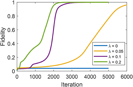
Figure 1. The optimization from an initial control field that traps the system at J = 0.04 in the absence of polarizability (λ = 0). The presence of the random polarizability term (see the text for further details) steers the optimization away from the trap.

4.2. The Effect of Adding a Polarizability Term to a System With a Second-Order Trap

In this section we assess the potential for the addition of a polarizability term to remove a trap from the landscape of a system known to possess one due to the loss of local controllability [i.e., violation of assumption (2) in section 2]. This example can be found in [6] [i.e., and in [30] where it is referred to as “system E”]:

$\begin{array}{l}{H}_0=\left[\begin{array}{ccc}1+\frac{\pi }{1000}& 0& 0\\ 0& 1& 0\\ 0& 0& 2\end{array}\right],H_1=\left[\begin{array}{ccc}-5\sqrt{\frac{2}{3}}& -1& 0\\ -1& -4& -1\\ 0& -1& -1\end{array}\right],\\ W=\left[\begin{array}{ccc}{e}^{i\frac{2\pi }{3}}& 0& 0\\ 0& -i{e}^{i\frac{3\pi }{4}}& 0\\ 0& 0& -i{e}^{i\varphi }\end{array}\right]exp(-i{H}_0·1000).& (16)\end{array}$

The field E = 0 is known to be a second order trap for this system.

We generated 1,000 random polarizability matrices H₂ ∈ 𝔲(3) ($\frac{1}{10}$ of the norm of H₁), and for each case a random initial field was generated in the vicinity of the zero field. It was found that, for initial fields arbitrarily close to the zero field, all gradient ascent runs converged to full fidelity. As such, we can conclude that the dipole trapping effect due to Equation (16) observed in [30] can be counteracted by the addition of a polarizability term.

4.3. Observed Properties of Generic Systems With a Polarizability Term

In this section, we assess if the addition of a polarizability term can introduce traps into the landscapes of systems known to have none in practice without a polarizability term; that is, each of the cases utilizes randomly chosen H₀ and H₁, which are known [31] to almost always produce trap free landscapes for W. All the cases here and in section 4.4 have n = 4 levels, unless otherwise stated. We numerically analyze the landscape of general systems of the form in Equation (3), which include polarizability. One thousand random tuples $(H_0,H_1,H_2,W=e^{iA})$ were generated and their landscapes similarly analyzed with 100 runs, each with a random initial field E(t). The real and imaginary elements of the complex Hermitian matrices H₀, H₁, H₂, and A were drawn separately from a uniform distribution over [−1, 1]. This procedure is used in the other studies below. The initial fields E(t) were uniformly and randomly generated to have E(t) ∈ [−1, 1] for all discretized components for t ∈ [0, T], but the components were unrestricted in magnitude during the optimization. The resultant landscapes were found to be trap free, as all runs converged within practical computational timescales to fidelity above 0.99.

The term H₂ typically has a norm which is less than H₁ in physical applications. In situations where a control is exploiting the effect of H₂ to achieve the implementation of a desired gate W, one might reasonably conjecture that a small size polarizability H₂ requires a very strong field or very high total field fluence. The fidelity is plotted along with the field fluence of E(t) in Figure 2 vs. algorithm iteration for three cases of 100 randomly generated tuples (H₀, H₁, H₂, W). In all cases the fidelity reached at least 0.99. The fluence of a field E is defined as:

$||E||=\frac{1}{T}{\displaystyle {\int }_0^T}{E}^2(t)dt.$

FIGURE 2

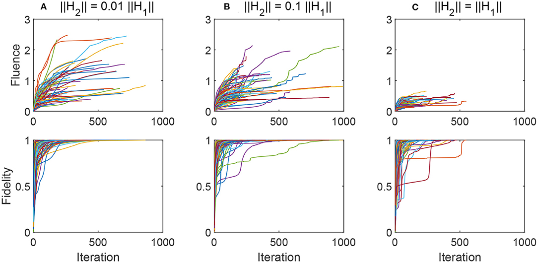
Figure 2. Fidelity and fluence ||E|| plotted verses algorithm iteration in three cases from weak to strong randomly chosen polarizability: (A) ||H₂|| ~ 0.01||H₁||, (B) ||H₂|| ~ 0.1||H₁||, and (C) ||H₂|| ~ ||H₁||.

All the simulations start from a small-fluence initial guess of the control field, and the fluence increases with iteration. When the polarization H₂ is weak (compared with the norm of H₁, as in Figures 2A,B, the fluence significantly increases with iteration, suggesting that the polarizability plays an important role requiring sufficient fluence. When H₁ and H₂ have the same norms (as in Figure 2C), the controls do not significantly increase in fluence with iteration. This case suggests that the effects of polarizability can be exploited for control without a significant rise in field amplitude over iteration. Moreover, in all cases and to some degree in Figure 1 the inflection points in the fidelity vs. iteration curves likely indicate that the climbing trajectories come near saddles, which are known to exist in the case of H = H₀ + E(t)H₁ and are expected to be present when H₂ is included.

4.4. The Neighborhood of Singular Controls

In this section, we explore the neighborhood of singular controls to check for trapping behavior in several types of systems. It is not known generally what proportion of singular controls are singular critical controls, and what proportion of singular critical controls are traps. Here we assess if singular controls play a significant role in determining the topology of critical points on quantum control landscapes for systems with a polarizability term present. Following the work in [11], one can numerically solve the Schrödinger equation to obtain singular controls E(t). This can be achieved by substituting Equation (10) into Equation (3) and then substituting the resulting Hamiltonian into Equation (2) to obtain the initial value problem (i.e., in Equation 17) it is understood that E(t) is given by Equation (10), thereby making Equation (17) highly non-linear in U(t):

$\begin{array}{ll}\dot{U}(t)=-i\left[H_0+E(t)H_1+E^2(t)H_2\right]U(t),U(0)=I.& (17)\end{array}$

A solution U(t) to this system of equations is a singular trajectory emanating from the group identity at t = 0. Equation (10) shows that the set of all singular trajectories is parameterized by B ∈ 𝔰𝔲(n). From a numerical solution of Equation (17), the corresponding singular control can be obtained by substituting the singular trajectory U(t) into Equation (10).

In order to test if any given singular control E is a trap, it is possible to explore the neighborhood of E by evaluating F[E+δE] for many small δE and assessing the sign of δF = F[E+δE]−F[E]. If two linearly independent δE can be found such that δF has different signs (i.e., one positive and one negative) then the point E must be a saddle in control space rather than a trap. Two types of systems were assessed in this respect.

In the first scenario 10,000 tuples (H₀, H₁, H₂, B, W) were uniformly and randomly generated, as previously described, and the corresponding singular control was found numerically by solving Equation (17) in order to obtain a singular trajectory and thus, in turn generate a singular control from Equation (10). In all cases, no traps were found, as an average of 3.23 variations δE of the control were required to identify two which resulted in fidelity variations of opposite sign. Furthermore, the highest number of trial variations required for any singular control was 70. This behavior indicates that all of the singular controls examined are saddles on the control landscape.

The second class of Hamiltonians assessed were those in Equations (14) and (15) with n = 5 for H₀ and H₁. Ten thousand tuples (H₂, B, W) were generated uniformly at random and the corresponding singular control was found numerically by solving Equation (17) in order to obtain a singular trajectory and thus a singular control, as before. In all cases, no trapping behavior was found, and the highest number of trial variations required for assessing the nature of any singular control was 200. This again indicates that all of the singular controls examined are saddles on the control landscape, even when the landscape derived from H = H₀ + E(t)H₁, which produces at least one trap (i.e., see the discussion in section 4.1).

From these cases upon visual examination of many singular controls, they can be seen to exhibit characteristic features. Most notably, there are two distinct classes. The dominant first class are all physically plausible fields as they are smooth and bounded. Controls in the second class all possess at least one blow-up point where the control becomes both unbounded and discontinuous (i.e., they possess infinite jump discontinuities, similar to the reciprocal function $f(x)=\frac{1}{x}$ at x = 0), as such, they are clearly excluded from physical consideration. This behavior arises from the denominator in Equation (10) passing through zero. The comments below Equation (10) explain how to deal with this behavior, but it was not explored in the simulations here.

For each matrix B ∈ 𝔰𝔲(4), there is a singular control defined by Equations (17) and (10). Using randomized gradient decent for B, we can produce singular critical controls, rather than just singular ones. We thus optimize over B such that it is co-linear to $U^{†}(T)\nabla J{|}_{U(T)}$ (to a numerical tolerance of 0.001 radians). For all cases, U(T) was not found to be a kinematic critical point of J(U(T)). In the case of 𝔰𝔲(4), this procedure consists of minimization over the 15 parameters of 𝔰𝔲(4). One parameter can be discarded as the formula for a singular control in Equation (10) doesn't depend on the norm of B due to the linearity of the numerator and denominator in B. Thus, it is possible to restrict the search to the unit norm of B. We found that this search did not always succeed in finding a singular critical control; only about 5% of searches succeeded. This suggests that the set of singular critical controls is very small in the set of singular controls.

In order to explore the latter prospect, we studied the structure of the control landscape in systems with randomly generated tuples (H₀, H₁, H₂, B, W) as before. We analyzed the possibility of whether a singular critical control E is a trap on the control landscape of F by making many small variations E′ : = E + δE around E. For each E′ a randomized gradient ascent was initiated. If a singular critical E were a true trap, rather than a saddle, this would be identified by at least some gradient ascent runs returning back to E (or a control near to E of the same fidelity) when initiated from E + δE. If full fidelity was reached during the run, then E cannot be a trap. One hundred tuples (H₀, H₁, H₂, B, W) were generated and for each tuple 100 singular critical controls were created as described in the last paragraph. For each singular critical control E, 200 points E′ in the neighborhood of E were generated and an associated gradient-ascent run was completed. The norm of δE was chosen to be random within [0, 0.001] (which is typically very small compared to the norm of E(t)) so as to ensure exploring close to the candidate trap and the behavior around it. We found that all runs converged to F[E] ≃ 1.0 and displayed similar convergence rates as those cases seen when initial controls were chosen at random from the whole control space. Lastly, the singular critical controls generally exhibited no clear visually differentiating features when compared to the singular, non-critical controls. As such, no example is shown; also see the remarks earlier in this section regarding the denominator in Equation (10).

5. Conclusions, Outlook, and Further Studies

We have shown that upon including a polarizability term in the Hamiltonian, and thus moving beyond the standard dipole approximation, a change in the character of quantum control landscapes is seen in some relevant n = 3, 4, and 5 level cases. We have also shown that there is a theoretical difference between the nature for the singular controls in the cases with and without the polarizability term.

There are two central conclusions from this work:

1. Including a polarizability term H₂ does not introduce traps into the landscape for typical tuples (H₀, H₁, H₂, W).

2. Including a random polarizability term can remove traps from the landscapes for a class of otherwise uncontrollable systems based upon H₀ and H₁, including the situation of a trap at zero field.

It has been shown that almost all Hamiltonians based up on H₀ and H₁ do not correspond to traps in quantum control landscapes with the exceptions forming a null set of systems [31]. However, this result does not exclude exceptions to particularly violating assumptions (1) or (2) of section 2. Concerning satisfaction of global or local controllablity, this paper considered a few known exceptions and showed that the addition of a random H₂ term returned the augmented system to normal behavior [i.e., the original (H₀, H₁) driven traps were removed].

In this work for systems based on arbitrary (H₀, H₁, H₂, B, W), an algorithm was devised to search for singular critical controls and analyze if they are traps by examining F in a neighborhood of any discovered singular critical controls. Effectively, this process is exploring the nature of the eigenvalues of the Hessian of the end-point map (i.e., and possibly the impact of higher order derivatives of F[E] playing a role) at the singular critical points. In [11] no trapping singular controls were found in the case of linear coupling H₁ and the control of the density matrix. Our work extends this finding in two respects. Firstly, we study the control of the full quantum propagator U(t). Secondly, we study the role of non-linear polarizability coupling H₂ along with H₁. Future work should include repeating the numerical analysis of [11] in the case of the control of the density matrix and the observable maximization task for systems with a polarizability term and even higher order coupling terms in the Hamiltonian.

This work provides numerical evidence to bolster the claim that trap free landscapes are ubiquitous in the practice of quantum control. We conjecture that including more terms and their tensor character in the expansion in Equation (4) will have the general effect of removing traps from the landscape by adding novel dynamical mechanisms induced by the controls via couplings to an external field or fields (in the case of tensor H_k). This conjecture simply states that nominal system “complexity” aids in increasing the likelihood that assumptions (1) and (2) will hold, naturally assuming that adequate resources are available for this purpose [i.e., satisfaction of assumption (3)]. An assessment of this conjecture should form the basis for further analytical and numerical investigation. A possible path to proving this conjecture may lie in combining the proof of global controllability [27] with an extension of local controllability [41]. Importantly, in the laboratory with atoms and molecules additional terms beyond the dipole approximation will inherently be present, even if they are weak. In summary, this work goes beyond the majority of theoretical studies in quantum control and quantum control landscapes, which investigate systems restricted to the dipole approximation. The tantalizing numerical findings in the paper and the generic existence of molecular polarization warrants an assessment of the physical conjecture made above, which may be captured by the statement that system complexity appears to be a friend for finding favorable control landscape topology.

Data Availability Statement

The original contributions presented in the study are included in the article, further inquiries can be directed to the corresponding author.

Author Contributions

BR, R-BW, and HR contributed to conception and design of the study. BR performed the simulation, analysis, and composition. R-BW checked the simulation and help editing the paper. HR proposed the main idea and edit the paper. All authors contributed to the article and approved the submitted version.

Funding

HR acknowledges support from the US ARO (W911NF-19-1-0382) and BR acknowledges support from the US DOE (DE-FG02-02ER15344).

Conflict of Interest

The authors declare that the research was conducted in the absence of any commercial or financial relationships that could be construed as a potential conflict of interest.

References

1. Chakrabarti, Rabitz H. Quantum control landscapes. Int Rev Phys Chem. (2007) 26:671–735. doi: 10.1080/01442350701633300

CrossRef Full Text | Google Scholar

2. Judson RS, Rabitz H. Teaching lasers to control molecules. Phys Rev Lett. (1992) 68:1500–3. doi: 10.1103/PhysRevLett.68.1500

PubMed Abstract | CrossRef Full Text | Google Scholar

3. Rabitz H, de Vivie-Riedle R, Motzkus M, Kompa K. Whither the future of controlling quantum phenomena? Science. (2000) 288:824–8. doi: 10.1126/science.288.5467.824

PubMed Abstract | CrossRef Full Text | Google Scholar

4. Pechen AN, Tannor DJ. Are there traps in quantum control landscapes? Phys Rev Lett. (2011) 106:120402. doi: 10.1103/PhysRevLett.106.120402

PubMed Abstract | CrossRef Full Text | Google Scholar

5. Rabitz H, Ho TS, Long R, Wu R, Brif C. Comment on “Are There Traps in Quantum Control Landscapes?”. Phys Rev Lett. (2012) 108:198901. doi: 10.1103/PhysRevLett.108.198901

PubMed Abstract | CrossRef Full Text | Google Scholar

6. De Fouquieres P, Schirmer SG. A closer look at quantum control landscapes and their implication for control optimization. Infinite Dimens Anal Quant Probabil Relat Top. (2013) 16:1350021. doi: 10.1142/S0219025713500215

CrossRef Full Text | Google Scholar

7. Roslund J, Rabitz H. Experimental quantum control landscapes: inherent monotonicity and artificial structure. Phys Rev A. (2009) 80:013408. doi: 10.1103/PhysRevA.80.013408

CrossRef Full Text | Google Scholar

8. Roslund J, Rabitz H. Gradient algorithm applied to laboratory quantum control. Phys Rev A. (2009) 79:053417. doi: 10.1103/PhysRevA.79.053417

CrossRef Full Text | Google Scholar

9. Palao JP, Kosloff R. Quantum computing by an optimal control algorithm for unitary transformations. Phys Rev Lett. (2002) 89:188301. doi: 10.1103/PhysRevLett.89.188301

PubMed Abstract | CrossRef Full Text | Google Scholar

10. Caneva T, Murphy M, Calarco T, Fazio R, Montangero S, Giovannetti V, et al. Optimal control at the quantum speed limit. Phys Rev Lett. (2009) 103:240501. doi: 10.1103/PhysRevLett.103.240501

PubMed Abstract | CrossRef Full Text | Google Scholar

11. Wu RB, Long R, Dominy J, Ho TS, Rabitz H. Singularities of quantum control landscapes. Phys Rev A. (2012) 86:013405. doi: 10.1103/PhysRevA.86.013405

CrossRef Full Text | Google Scholar

12. Moore KW, Rabitz H. Exploring quantum control landscapes: topology, features, and optimization scaling. Phys Rev A. (2011) 84:012109. doi: 10.1103/PhysRevA.84.012109

CrossRef Full Text | Google Scholar

13. Moore KW, Rabitz H. Exploring constrained quantum control landscapes. J Chem Phys. (2012) 137:134113. doi: 10.1063/1.4757133

PubMed Abstract | CrossRef Full Text | Google Scholar

14. Nuernberger P, Vogt G, Brixner T, Gerber G. Femtosecond quantum control of molecular dynamics in the condensed phase. Phys Chem Chem Phys. (2007) 9:2470–97. doi: 10.1039/b618760a

PubMed Abstract | CrossRef Full Text | Google Scholar

15. Levis RJ, Rabitz HA. Closing the loop on bond selective chemistry using tailored strong field laser pulses. J Phys Chem A. (2002) 106:6427–44. doi: 10.1021/jp0134906

CrossRef Full Text | Google Scholar

16. Herek JL, Wohlleben W, Cogdell RJ, Zeidler D, Motzkus M. Quantum control of energy flow in light harvesting. Nature. (2002) 417:533–5. doi: 10.1038/417533a

PubMed Abstract | CrossRef Full Text | Google Scholar

17. Timoney N, Elman V, Glaser S, Weiss C, Johanning M, Neuhauser W, et al. Error-resistant single-qubit gates with trapped ions. Phys Rev A. (2008) 77:052334. doi: 10.1103/PhysRevA.77.052334

CrossRef Full Text | Google Scholar

18. Lucero E, Kelly J, Bialczak RC, Lenander M, Mariantoni M, Neeley M, et al. Reduced phase error through optimized control of a superconducting qubit. Phys Rev A. (2010) 82:042339. doi: 10.1103/PhysRevA.82.042339

CrossRef Full Text | Google Scholar

19. Arute F, Arya K, Babbush R, Bacon D, Bardin JC, Barends R, et al. Quantum supremacy using a programmable superconducting processor. Nature. (2019) 574:505–10. doi: 10.1038/s41586-019-1666-5

PubMed Abstract | CrossRef Full Text | Google Scholar

20. Lapert M, Zhang Y, Braun M, Glaser SJ, Sugny D. Singular extremals for the time-optimal control of dissipative spin $\frac{1}{2}$ particles. Phys Rev Lett. (2010) 104:083001. doi: 10.1103/PhysRevLett.104.083001

PubMed Abstract | CrossRef Full Text | Google Scholar

21. Applequist J, Carl JR, Fung KK. Atom dipole interaction model for molecular polarizability. Application to polyatomic molecules and determination of atom polarizabilities. J Am Chem Soc. (1972) 94:2952–60. doi: 10.1021/ja00764a010

CrossRef Full Text | Google Scholar

22. Kaminski GA, Stern HA, Berne BJ, Friesner RA. Development of an accurate and robust polarizable molecular mechanics force field from ab initio quantum chemistry. J Phys Chem A. (2004) 108:621–7. doi: 10.1021/jp0301103

CrossRef Full Text | Google Scholar

23. Fu H, Schirmer SG, Solomon AI. Complete controllability of finite-level quantum systems. J Phys A Math Gen. (2001) 34:1679. doi: 10.1088/0305-4470/34/8/313

CrossRef Full Text | Google Scholar

24. Dominy J, Rabitz H. Dynamic homotopy and landscape dynamical set topology in quantum control. J Math Phys. (2012) 53:082201. doi: 10.1063/1.4742375

CrossRef Full Text | Google Scholar

25. Grigoriu A. Stability analysis of discontinuous quantum control systems with dipole and polarizability coupling. Automatica. (2012) 48:2229–34. doi: 10.1016/j.automatica.2012.06.028

CrossRef Full Text | Google Scholar

26. Coron JM, Grigoriu A, Lefter C, Turinici G. Quantum control design by Lyapunov trajectory tracking for dipole and polarizability coupling. N J Phys. (2009) 11:105034. doi: 10.1088/1367-2630/11/10/105034

CrossRef Full Text | Google Scholar

27. Turinici G. Beyond bilinear controllability: applications to quantum control. In: Kunisch K, Sprekels J, Leugering G, Tröltzsch F, editors. Control of Coupled Partial Differential Equations. Basel: Birkhäuser Basel (2007). p. 293–309. doi: 10.1007/978-3-7643-7721-2_13

CrossRef Full Text | Google Scholar

28. Verbiest T, Clays K, Samyn C, Wolff J, Reinhoudt D, Persoons A. Investigations of the hyperpolarizability in organic molecules from dipolar to octopolar systems. J Am Chem Soc. (1994) 116:9320–23. doi: 10.1021/ja00099a058

CrossRef Full Text | Google Scholar

29. Long R, Riviello G, Rabitz H. The gradient flow for control of closed quantum systems. IEEE Trans Automat Control. (2013) 58:2665–9. doi: 10.1109/TAC.2013.2256677

CrossRef Full Text | Google Scholar

30. Riviello G, Brif C, Long R, Wu RB, Tibbetts KM, Ho TS, et al. Searching for quantum optimal control fields in the presence of singular critical points. Phys Rev A. (2014) 90:013404. doi: 10.1103/PhysRevA.90.013404

CrossRef Full Text | Google Scholar

31. Russell B, Rabitz H, Wu RB. Control landscapes are almost always trap free: a geometric assessment. J Phys A Math Theoret. (2017) 50:205302. doi: 10.1088/1751-8121/aa6b77

CrossRef Full Text | Google Scholar

32. Altafini C. Controllability of quantum mechanical systems by root space decomposition of su(N). J Math Phys. (2002) 43:2051. doi: 10.1063/1.1467611

CrossRef Full Text | Google Scholar

33. Wu RB, Hsieh MA, Rabitz H. Role of controllability in optimizing quantum dynamics. Phys Rev A. (2011) 83:062306. doi: 10.1103/PhysRevA.83.062306

CrossRef Full Text | Google Scholar

34. Pechen A, Il'in N. Trap-free manipulation in the Landau-Zener system. Phys Rev A. (2012) 86:052117. doi: 10.1103/PhysRevA.86.052117

CrossRef Full Text | Google Scholar

35. Pechen AN, Il'in NB. Coherent control of a qubit is trap-free. Proc Steklov Instit Math. (2014) 285:233–40. doi: 10.1134/S0081543814040166

CrossRef Full Text | Google Scholar

36. Zhdanov DV. Comment on ‘Control landscapes are almost always trap free: a geometric assessment’. J Phys A Math Theoret. (2018) 51:508001. doi: 10.1088/1751-8121/aaecf6

CrossRef Full Text | Google Scholar

37. Russell B, Wu RB, Rabitz H. Reply to comment on ‘control landscapes are almost always trap free: a geometric assessment’. J Phys A Math Theoret. (2018) 51:508002. doi: 10.1088/1751-8121/aaecf2

CrossRef Full Text | Google Scholar

38. Jost J, Li-Jost X. Calculus of Variations. Cambridge, UK: Cambridge University Press (1998).

Google Scholar

39. Sussmann HJ, editor. Nonlinear Controllability and Optimal Control. New York, NY: Chapman & Hall/CRC Pure and Applied Mathematics; Taylor & Francis; (1990).

Google Scholar

40. Rowland B, Jones JA. Implementing quantum logic gates with gradient ascent pulse engineering: principles and practicalities. Philos Trans R Soc A. (2012). 370:4636–50. doi: 10.1098/rsta.2011.0361

PubMed Abstract | CrossRef Full Text | Google Scholar

41. Russell B, Vuglar S, Rabitz H. Control landscapes for a class of non-linear dynamical systems: sufficient conditions for the absence of traps. J Phys A Math Theoret. (2018) 51:335103. doi: 10.1088/1751-8121/aacc85

CrossRef Full Text | Google Scholar