Diverse Novel Stable Traveling Wave Solutions of the Advanced or Voltage Spectrum of Electrified Transmission Through Fractional Non-linear Model

This study analyzes the exact solutions of the compliance fractional non-linear time–space telegraph (FNLTST) equation by Oliver Heaviside in 1880 via three non-applied analytical schemes. The solutions obtained to define the advanced or voltage spectrum of electrified transmission with day-to-day distance from electrical communication or the application of electromagnetic waves. Many new solutions are obtained, and three distinct styles of drawings are introduced (two-dimensional, three-dimensional, and density plots). Furthermore, stability characterization of the solutions is addressed using the properties of the Hamiltonian system. The originality of this study is shown by matching the solutions built with solutions produced previously using various analytical methods. Overall, the success of the three systems demonstrates their quality, intensity, and capacity to cope with several different types of non-linear evolutionary equations.

1. Introduction

The new generators of complicated systems, namely infectious disease epidemiology [1], neural network [2], genetics [3], fluid mechanic [4], community ecology [5], Solid-State Physics [6], plasma wave spread [7], thermodynamics [8], matter condensation [9], non-linear optimal [10], were employed. Formulating these phenomena through non-linear evolution equations relies on real testing to define parameters and to provide empirically unmistakable evidence that describes the intricate mechanisms of their physical and dynamic actions [11–13]. This implies that the key activity of these models is specified as functions, while the success factors for this behavior become [14] parameters. Many separate mathematicians and physicists also concentrate extensively on researching these mathematical models to understand more about their undiscovered properties [15, 16]. On the other hand, computational, analytical, and semi-analytical structures have been derived from fulfilling the same function [17–20].

Nowadays, fractional computation receives great attention in several science branches as it is able to discuss the non-local property of the mathematical models in detail [21, 22]. Thus, many fractional derivative operators have been derived to convert the non-linear partial differential equations into the ordinary differential equations, such as Riemann–Liouville, Caputo, the conformal fractional, and Atangana–Baleanu derivative operators [23–26]. These fractional operators have been employed for several non-linear evolution equations and have proved their effectiveness and powerfulness [27, 28].

This study handles a fundamental non-linear construction equation in electromagnetic waves, namely the compatible non-linear time-space equation. This equation model illustrates the advanced or voltage spectrum of an electrical transmission range with day-to-day distance from the electrical or wave application. This model is given mathematically by [29–31]

$\begin{array}{ll}{D}_{tt}^{2\alpha }{V}-D_{xx}^{2\alpha }{V}+D_t^{\alpha }{V}+b{V}+d{{V}}^3=0,0<\alpha \le 1,& (1)\end{array}$

where b, d are arbitrary constants to be evaluated through the considered analytical schemes. Mixing between conformable fractional derivative and traveling wave transformation as following ${V}(x,t)={Q}(\Xi ),\Xi =\frac{a{x}^{\alpha }}{\alpha }-\frac{c{t}^{\alpha }}{\alpha }$, where a, c are arbitrary constants, and using it along with Equation (1) converts the non-linear partial differential equation (NLPDE) into the next ordinary differential equation (ODE).

$\begin{array}{ll}(c^2-a^2){{Q}}^{″}-c{{Q}}^{\prime }+b{Q}+d{{Q}}^3=0.& (2)\end{array}$

Using the homogeneous balance principle along the auxiliary equation of extended simplest equation method [32–35] $[{\Phi }^{\prime }(\Xi )={\alpha }_{\ast }+\lambda \Phi (\Xi )+\mu \Phi {(\Xi )}^2]$, with n = 1, where n is the obtained value of homogeneous principle between the highest order derivative term and non-linear term in Equation (2), we get the following $[{{Q}}^{″}\&{{Q}}^3\mapsto n+2=3n]$.

The section of the rest of the study are ordered as follows: in section 2, the above analytical schemes [32–35] are employed to achieve the solitary solution of the non-linear fractional time-space equation. Besides, the dynamical behavior of the solutions obtained is investigated through two-dimensional, three-dimensional, and density plots. The originality of the research is clarified in section 3. The conclusion of the entire study is presented in section 4.

2. Solitary Wave Solutions

In this section, the solitary wave solutions of fractional non-linear time–space telegraph (FNLTST) equation are investigated through the abovementioned computational schemes as following:

2.1. Extended Sech–Tanh Expansion Method's Solution

The general solution of the FNLTST equation is formulated by the suggested structure and measured balance value by

$\begin{array}{l}{Q}(\Xi )={\displaystyle \sum _{i=1}^n}{\text{sech}}^{i-1}(\Xi )(a_i\text{sech}(\Xi )+b_{i}tanh(\Xi ))\\ +a_0=a_1\text{sech}(\Xi )+a_0+b_{1}tanh(\Xi ),& (3)\end{array}$

where a₀, a₁, and b₁ are arbitrary constants to be determined later. Using the framework of the suggested method, produces the value of above-shown parameters is given as follows

$\begin{array}{r}{a}_0=-\frac{\sqrt{b}}{2\sqrt{d}},a_1=0,b_1=-\frac{\sqrt{b}}{2\sqrt{d}},c=\frac{3b}{4},\\ a=-\frac{1}{4}\sqrt{b}\sqrt{9b-2},\text{where }(b>\frac{2}{9}\&d>0).\end{array}$

Hence, the solutions of Equation (1) in the next form is

$\begin{array}{ll}{{V}}_1(x,t)=\frac{1}{2}\sqrt{\frac{b}{d}}\left(tanh\left(\frac{3b{t}^{\alpha }+\sqrt{b}\sqrt{9b-2}{x}^{\alpha }}{4\alpha }\right)-1\right).& (4)\end{array}$

2.2. The Solutions of Extended sinh-Gordon Equation Expansion Method

The general solution of the FNLTST equation is formulated by the suggested structure and the measured balance value by

$\begin{array}{ll}\begin{array}{c}{V}(\Xi )={\displaystyle \sum _{i=0}^n}{cosh}^{i-1}(w(\Xi ))(A_{i}cosh(w(\Xi ))+B_{i}sinh(w(\Xi )))\\ +A_0=A_{1}cosh(w(\Xi ))+A_0+B_{1}sinh(w(\Xi )),\end{array}& (5)\end{array}$

where A₀, A₁, and B₁ are arbitrary constants to be evaluated later. Using the framework of the suggested method, the value of above shown parameters can be obtained as follows

Case 1. For w′(θ) = sinh(θ) and by substituting Equation (5) and its derivatives into Equation (2) in the framework of the suggested scheme, we obtained the following values of the abovementioned arbitrary constants:

Family I.

$\begin{array}{r}{A}_0=\frac{\sqrt{-b}}{2\sqrt{d}},A_1=-\frac{\sqrt{-b}}{2\sqrt{d}},B_1=0,a=-\frac{1}{4}\sqrt{b}\sqrt{9b-2},\\ c=\frac{3b}{4},\text{where }d<0\&b>\frac{2}{9}.\end{array}$

Hence, the solutions of Equation (1) take the next forms

$\begin{array}{ll}{{V}}_2(x,t)=\frac{-1}{2}\sqrt{\frac{-b}{d}}\left(tanh\left(\frac{3b{t}^{\alpha }+\sqrt{b}\sqrt{9b-2}{x}^{\alpha }}{4\alpha }\right)-1\right),& (6)\end{array}$

$\begin{array}{ll}{{V}}_3(x,t)=\frac{-1}{2}\sqrt{\frac{-b}{d}}\left(coth\left(\frac{3b{t}^{\alpha }+\sqrt{b}\sqrt{9b-2}{x}^{\alpha }}{4\alpha }\right)-1\right).& (7)\end{array}$

Family II.

$\begin{array}{r}{A}_0=0,A_1=0,B_1=-\frac{\sqrt{2b-1}}{\sqrt{d}},a=-\frac{\sqrt{2b-1}}{\sqrt{2}},\\ c=1\text{where }(d>0\&\frac{1}{2}\ne b>0).\end{array}$

Thus, the solutions of Equation (1) are constructed by

$\begin{array}{ll}{{V}}_4(x,t)=-\sqrt{\frac{1-2b}{d}}\text{sech}\left(\frac{\sqrt{2b-1}{x}^{\alpha }}{\sqrt{2}\alpha }+\frac{t^{\alpha }}{\alpha }\right),& (8)\end{array}$

$\begin{array}{ll}{{V}}_5\left(x,t\right)=-\sqrt{\frac{1-2b}{d}}\text{csch}\left(\frac{\sqrt{2b-1}{x}^{\alpha }}{\sqrt{2}\alpha }+\frac{t^{\alpha }}{\alpha }\right).& (9)\end{array}$

Family III.

$\begin{array}{r}{A}_0=\frac{-1}{2}\sqrt{\frac{-b}{d}},A_1=\frac{-1}{2}\sqrt{\frac{-b}{d}},B_1=0,a=-\frac{1}{4}\sqrt{b}\sqrt{9b-2},\\ c=-\frac{3b}{4},\text{where }\left(b<0\&d>0\right).\end{array}$

Therefore, the solutions of Equation (1) are given by

$\begin{array}{ll}{{V}}_6\left(x,t\right)=\frac{1}{2}\sqrt{\frac{-b}{d}}\left(tanh\left(\frac{3b{t}^{\alpha }-\sqrt{b}\sqrt{9b-2}{x}^{\alpha }}{4\alpha }\right)-1\right),& (10)\end{array}$

$\begin{array}{ll}{{V}}_7\left(x,t\right)=\frac{1}{2}\sqrt{\frac{-b}{d}}\left(coth\left(\frac{3b{t}^{\alpha }-\sqrt{b}\sqrt{9b-2}{x}^{\alpha }}{4\alpha }\right)-1\right).& (11)\end{array}$

Case 2. For w′(θ) = cosh(θ) and by substituting Equation (5) and its derivatives into Equation (2) in the framework of the suggested scheme, we obtained the following values of the abovementioned arbitrary constants:

Family I.

$\begin{array}{r}{A}_0=-\frac{i\sqrt{b}}{2\sqrt{d}},A_1=0,B_1=-\frac{\sqrt{b}}{2\sqrt{d}},a=-\frac{1}{4}\sqrt{2b-9b^2},\\ c=\frac{3ib}{4},\text{where}\left(d<0,i=\sqrt{-1}\right).\end{array}$

Thus, the solutions of Equation (1) take the following formulas

$\begin{array}{ll}{{V}}_8\left(x,t\right)=\frac{1}{2}\sqrt{\frac{-b}{d}}\left(-1+tanh\left(\frac{3b{t}^{\alpha }-\sqrt{\left(9b-2\right)b}{x}^{\alpha }}{4\alpha }\right)\right),& (12)\end{array}$

$\begin{array}{ll}{{V}}_9\left(x,t\right)=\frac{1}{2}\sqrt{\frac{-b}{d}}\left(-1+coth\left(\frac{3b{t}^{\alpha }-\sqrt{\left(9b-2\right)b}{x}^{\alpha }}{4\alpha }\right)\right).& (13)\end{array}$

Family II.

$\begin{array}{r}{A}_0=-\frac{i\sqrt{b}}{2\sqrt{d}},A_1=-\frac{\sqrt{b}}{2\sqrt{d}},B_1=-\frac{\sqrt{b}}{2\sqrt{d}},\\ a=-\frac{1}{2}\sqrt{2b-9b^2},c=\frac{3ib}{2},\text{where}\left(d<0,i=\sqrt{-1}\right).\end{array}$

Hence, the solutions of Equation (1) are formulated in the following forms

$\begin{array}{l}{{V}}_{10}\left(x,t\right)=(\frac{1}{2}\sqrt{\frac{-b}{d}}tanh\left(\frac{3b{t}^{\alpha }}{2\alpha }-\frac{\sqrt{9b^2-2b}{x}^{\alpha }}{2\alpha }\right)\\ \mp \frac{1}{2}\sqrt{\frac{b}{d}}\text{sech}\left(\frac{3b{t}^{\alpha }}{2\alpha }-\frac{\sqrt{9b^2-2b}{x}^{\alpha }}{2\alpha }\right))-\frac{1}{2}\sqrt{\frac{-b}{d}},& (14)\end{array}$

$\begin{array}{l}{{V}}_{11}\left(x,t\right)=(\frac{1}{2}\sqrt{\frac{-b}{d}}coth\left(\frac{3b{t}^{\alpha }}{2\alpha }-\frac{\sqrt{9b^2-2b}{x}^{\alpha }}{2\alpha }\right)\\ \mp \frac{1}{2}\sqrt{\frac{b}{d}}\text{csch}\left(\frac{3b{t}^{\alpha }}{2\alpha }-\frac{\sqrt{9b^2-2b}{x}^{\alpha }}{2\alpha }\right))-\frac{1}{2}\sqrt{\frac{-b}{d}}.& (15)\end{array}$

Family III.

$\begin{array}{r}{A}_0=\frac{-1}{2}\sqrt{\frac{-b}{d}},A_1=0,B_1=\frac{\sqrt{b}}{2\sqrt{d}},a=\frac{1}{4}\sqrt{2b-9b^2},\\ c=-\frac{3ib}{4},\text{ where }\left(d<0,b>\frac{2}{9}\right).\end{array}$

Hence, the solutions of Equation (1) are constructed by

$\begin{array}{ll}{{V}}_{12}\left(x,t\right)=\frac{1}{2}\sqrt{\frac{-b}{d}}tanh\left(\frac{3b{t}^{\alpha }}{4\alpha }-\frac{i\sqrt{2b-9b^2}{x}^{\alpha }}{4\alpha }\right)-\frac{1}{2}\sqrt{\frac{-b}{d}},& (16)\end{array}$

$\begin{array}{ll}{{V}}_{13}\left(x,t\right)=\frac{1}{2}\sqrt{\frac{-b}{d}}coth\left(\frac{3b{t}^{\alpha }}{4\alpha }-\frac{i\sqrt{2b-9b^2}{x}^{\alpha }}{4\alpha }\right)-\frac{1}{2}\sqrt{\frac{-b}{d}}.& (17)\end{array}$

2.3. Extended Simplest Equation Method's Solutions

The general solution of the FNLTST equation is formulated by the suggested structure and the measured balance value by

$\begin{array}{ll}{V}\left(\Xi \right)={\displaystyle \sum _{i=-n}^n}{a}_i\Phi {\left(\Xi \right)}^i=\frac{a_{-1}}{\Phi \left(\Xi \right)}+a_0+a_1\Phi \left(\Xi \right),& (18)\end{array}$

where a₋₁, a₀, and a₁ are arbitrary constants to be determined later, while Φ(Ξ) is the solution function of the next ODE

$\begin{array}{ll}{\Phi }^{\prime }\left(\Xi \right)={\alpha }_{\ast }+\lambda \Phi \left(\Xi \right)+\mu \Phi {\left(\Xi \right)}^2,& (19)\end{array}$

where α_∗, λ, and μ are arbitrary constants to be calculated later. Using the framework of the suggested method, gets the value of above shown parameters as follows:

Family I.

$\begin{array}{l}b=\frac{-2c^2}{9\left(a+c\right)\left(a-c\right)},d=\frac{{\left(3a^2\lambda -3c^2\lambda +c\right)}^2}{18{a_0}^2\left(a-c\right)\left(a+c\right)},\\ \mu =\frac{\left(3a^2\lambda -3c^2\lambda -c\right)\left(3a^2\lambda -3c^2\lambda +c\right)}{36{\alpha }_{\ast }{\left(a-c\right)}^2{\left(a+c\right)}^2},\end{array}$

$a_{-1}=0,a_1=\frac{a_0\left(3a^2\lambda -3c^2\lambda -c\right)}{6{\alpha }_{\ast }\left(a-c\right)\left(a+c\right)}.$

Hence, the solitary solutions of Equation (1) take the following formulas

When λ = 0,

for α_∗μ > 0, we obtain

$\begin{array}{l}{{V}}_{14}\left(x,t\right)=a_0\\ -\frac{a_{0}c\sqrt{\alpha \mu }}{6\mu {\alpha }_{\ast }\left(a-c\right)\left(a+c\right)}tan\left(\sqrt{{\alpha }_{\ast }\mu }\left(\frac{a{x}^{\alpha }}{\alpha }-\frac{c{t}^{\alpha }}{\alpha }+C\right)\right),& (20)\end{array}$

$\begin{array}{l}{{V}}_{15}\left(x,t\right)=a_0\\ -\frac{a_{0}c\sqrt{\alpha \mu }}{6\mu {\alpha }_{\ast }\left(a-c\right)\left(a+c\right)}cot\left(\sqrt{{\alpha }_{\ast }\mu }\left(\frac{a{x}^{\alpha }}{\alpha }-\frac{c{t}^{\alpha }}{\alpha }+C\right)\right).& (21)\end{array}$

for α_∗μ < 0, we obtain

$\begin{array}{l}{{V}}_{16}\left(x,t\right)=a_0-\frac{a_{0}c\sqrt{-\alpha \mu }}{6\mu {\alpha }_{\ast }\left(a-c\right)\left(a+c\right)}tanh(\sqrt{-{\alpha }_{\ast }\mu }(\frac{a{x}^{\alpha }}{\alpha }\\ -\frac{c{t}^{\alpha }}{\alpha })\mp \frac{ln\left(C\right)}{2}),& (22)\end{array}$

$\begin{array}{l}{{V}}_{17}\left(x,t\right)=a_0-\frac{a_{0}c\sqrt{-\alpha \mu }}{6\mu {\alpha }_{\ast }\left(a-c\right)\left(a+c\right)}coth(\sqrt{-{\alpha }_{\ast }\mu }(\frac{a{x}^{\alpha }}{\alpha }\\ -\frac{c{t}^{\alpha }}{\alpha })\mp \frac{ln\left(C\right)}{2}).& (23)\end{array}$

When α_∗ = 0,

for λ > 0, we obtain

$\begin{array}{ll}{{V}}_{18}\left(x,t\right)=a_0+\frac{a_0\lambda e^{\lambda \left(\frac{a{x}^{\alpha }}{\alpha }-\frac{c{t}^{\alpha }}{\alpha }+C\right)}\left(3a^2\lambda -3c^2\lambda -c\right)}{6\alpha \left(1-\mu e^{\lambda \left(\frac{a{x}^{\alpha }}{\alpha }-\frac{c{t}^{\alpha }}{\alpha }+C\right)}\right)\left(a-c\right)\left(a+c\right)}.& (24)\end{array}$

for λ < 0, we obtain

$\begin{array}{ll}{{V}}_{19}\left(x,t\right)=a_0-\frac{a_0\mu e^{\lambda \left(\frac{a{x}^{\alpha }}{\alpha }-\frac{c{t}^{\alpha }}{\alpha }+C\right)}\left(3a^2\lambda -3c^2\lambda -c\right)}{6\alpha \left(1+\mu e^{\lambda \left(\frac{a{x}^{\alpha }}{\alpha }-\frac{c{t}^{\alpha }}{\alpha }+C\right)}\right)\left(a-c\right)\left(a+c\right)}.& (25)\end{array}$

The general solutions has the next form:

When $4{\alpha }_{\ast }\mu >{\lambda }^2$ and μ > 0, we get

$\begin{array}{l}{{V}}_{20}\left(x,t\right)=a_0\\ +\frac{a_0\left(3a^2\lambda -3c^2\lambda -c\right)}{12\mu {\alpha }_{\ast }\left(a-c\right)\left(a+c\right)}\sqrt{4{\alpha }_{\ast }\mu -{\lambda }^2}\\ tan\left(\frac{\sqrt{4{\alpha }_{\ast }\mu -{\lambda }^2}}{2}\left(\frac{a{x}^{\alpha }}{\alpha }-\frac{c{t}^{\alpha }}{\alpha }+C\right)\right)-\lambda ,& (26)\end{array}$

$\begin{array}{l}{{V}}_{21}\left(x,t\right)=a_0\\ +\frac{a_0\left(3a^2\lambda -3c^2\lambda -c\right)}{12\mu {\alpha }_{\ast }\left(a-c\right)\left(a+c\right)}\sqrt{4{\alpha }_{\ast }\mu -{\lambda }^2}\\ cot\left(\frac{\sqrt{4{\alpha }_{\ast }\mu -{\lambda }^2}}{2}\left(\frac{a{x}^{\alpha }}{\alpha }-\frac{c{t}^{\alpha }}{\alpha }+C\right)\right)-\lambda .& (27)\end{array}$

When $4{\alpha }_{\ast }\mu >{\lambda }^2$ and μ < 0, we get

$\begin{array}{l}{{V}}_{22}\left(x,t\right)=a_0+\frac{a_0\left(3a^2\lambda -3c^2\lambda -c\right)}{12\mu {\alpha }_{\ast }\left(a-c\right)\left(a+c\right)}\sqrt{4{\alpha }_{\ast }\mu -{\lambda }^2}\\ tan\left(\frac{\sqrt{4{\alpha }_{\ast }\mu -{\lambda }^2}}{2}\left(\frac{a{x}^{\alpha }}{\alpha }-\frac{c{t}^{\alpha }}{\alpha }+C\right)\right)+\lambda ,& (28)\end{array}$

$\begin{array}{l}{{V}}_{23}\left(x,t\right)=a_0+\frac{a_0\left(3a^2\lambda -3c^2\lambda -c\right)}{12\mu {\alpha }_{\ast }\left(a-c\right)\left(a+c\right)}\sqrt{4{\alpha }_{\ast }\mu -{\lambda }^2}\\ cot\left(\frac{\sqrt{4{\alpha }_{\ast }\mu -{\lambda }^2}}{2}\left(\frac{a{x}^{\alpha }}{\alpha }-\frac{c{t}^{\alpha }}{\alpha }+C\right)\right)+\lambda .& (29)\end{array}$

Family II.

$\begin{array}{r}b=\frac{-2c^2}{9\left(a+c\right)\left(a-c\right)},d=\frac{2c^2}{9{a_0}^2\left(a-c\right)\left(a+c\right)},\\ \lambda =\frac{c}{3\left(a+c\right)\left(a-c\right)},{\alpha }_{\ast }=a_{-1}=0.\end{array}$

Hence, the solitary solutions of Equation (1) are constructed in the next forms

for λ > 0, as

$\begin{array}{ll}{{V}}_{24}\left(x,t\right)=a_0+\frac{a_1\lambda e^{\lambda \left(\frac{a{x}^{\alpha }}{\alpha }-\frac{c{t}^{\alpha }}{\alpha }+C\right)}}{1-\mu e^{\lambda \left(\frac{a{x}^{\alpha }}{\alpha }-\frac{c{t}^{\alpha }}{\alpha }+C\right)}}and& (30)\end{array}$

for λ < 0, as

$\begin{array}{ll}{{V}}_{25}\left(x,t\right)=a_0-\frac{a_1\mu e^{\lambda \left(\frac{a{x}^{\alpha }}{\alpha }-\frac{c{t}^{\alpha }}{\alpha }+C\right)}}{1+\mu e^{\lambda \left(\frac{a{x}^{\alpha }}{\alpha }-\frac{c{t}^{\alpha }}{\alpha }+C\right)}}.& (31)\end{array}$

Family III.

$\begin{array}{r}b=\frac{-2c^2}{9\left(a+c\right)\left(a-c\right)},d=2\frac{{\mu }^2\left(a^2-c^2\right)}{{a_1}^2},\\ \lambda =\frac{c}{3\left(a+c\right)\left(a-c\right)},{\alpha }_{\ast }=a_{-1}=0.\end{array}$

Hence, the solitary solutions of Equation (1) are given,

for λ > 0, as

$\begin{array}{ll}{{V}}_{26}\left(x,t\right)=a_0+\frac{a_1\lambda e^{\lambda \left(\frac{a{x}^{\alpha }}{\alpha }-\frac{c{t}^{\alpha }}{\alpha }+C\right)}}{1-\mu e^{\lambda \left(\frac{a{x}^{\alpha }}{\alpha }-\frac{c{t}^{\alpha }}{\alpha }+C\right)}}and& (32)\end{array}$

for λ < 0, as

$\begin{array}{ll}{{V}}_{27}\left(x,t\right)=a_0-\frac{a_1\mu e^{\lambda \left(\frac{a{x}^{\alpha }}{\alpha }-\frac{c{t}^{\alpha }}{\alpha }+C\right)}}{1+\mu e^{\lambda \left(\frac{a{x}^{\alpha }}{\alpha }-\frac{c{t}^{\alpha }}{\alpha }+C\right)}}.& (33)\end{array}$

Family IV.

$\begin{array}{l}\alpha =\frac{\left(3a^2\lambda -3c^2\lambda -c\right)\left(3a^2\lambda -3c^2\lambda +c\right)}{36\mu {\left(a-c\right)}^2{\left(a+c\right)}^2},\\ b=\frac{-2c^2}{9\left(a+c\right)\left(a-c\right)},d=\frac{{\left(3a^2\lambda -3c^2\lambda -c\right)}^2}{18{a_0}^2\left(a-c\right)\left(a+c\right)},\\ a_{-1}=\frac{a_0\left(3a^2\lambda -3c^2\lambda +c\right)}{6\mu \left(a-c\right)\left(a+c\right)},a_1=0.\end{array}$

Hence, the solitary solutions of Equation (1) are evaluated in the following formulas:

When λ = 0,

for α_∗μ > 0, we obtain

$\begin{array}{l}{{V}}_{28}\left(x,t\right)=\\ \frac{a_{0}c}{6\sqrt{{\alpha }_{\ast }\mu }\left(a-c\right)\left(a+c\right)tan\left(\sqrt{{\alpha }_{\ast }\mu }\left(\frac{a{x}^{\alpha }}{\alpha }-\frac{c{t}^{\alpha }}{\alpha }+C\right)\right)}+a_0,& (34)\end{array}$

$\begin{array}{l}{{V}}_{29}\left(x,t\right)=\\ \frac{a_{0}c}{6\sqrt{{\alpha }_{\ast }\mu }\left(a-c\right)\left(a+c\right)cot\left(\sqrt{{\alpha }_{\ast }\mu }\left(\frac{a{x}^{\alpha }}{\alpha }-\frac{c{t}^{\alpha }}{\alpha }+C\right)\right)}+a_0.& (35)\end{array}$

for α_∗μ < 0, we obtain

$\begin{array}{l}{{V}}_{30}\left(x,t\right)=\\ \frac{a_{0}c}{6\sqrt{-{\alpha }_{\ast }\mu }\left(a-c\right)\left(a+c\right)tanh\left(\sqrt{-{\alpha }_{\ast }\mu }\left(\frac{a{x}^{\alpha }}{\alpha }-\frac{c{t}^{\alpha }}{\alpha }\right)\mp \frac{ln\left(C\right)}{2}\right)}+a_0,& (36)\end{array}$

$\begin{array}{l}{{V}}_{31}\left(x,t\right)=\\ \frac{a_{0}c}{6\sqrt{-{\alpha }_{\ast }\mu }\left(a-c\right)\left(a+c\right)coth\left(\sqrt{-{\alpha }_{\ast }\mu }\left(\frac{a{x}^{\alpha }}{\alpha }-\frac{c{t}^{\alpha }}{\alpha }\right)\mp \frac{ln\left(C\right)}{2}\right)}+a_0.& (37)\end{array}$

When α_∗ = 0,

for λ > 0, we obtain

$\begin{array}{ll}{{V}}_{32}\left(x,t\right)=\frac{a_0\left(3a^2\lambda -3c^2\lambda +c\right)\left(1-\mu e^{\lambda \left(\frac{a{x}^{\alpha }}{\alpha }-\frac{c{t}^{\alpha }}{\alpha }+C\right)}\right)}{6\mu \left(a-c\right)\left(a+c\right)\left(\lambda e^{\lambda \left(\frac{a{x}^{\alpha }}{\alpha }-\frac{c{t}^{\alpha }}{\alpha }+C\right)}\right)}+a_0.& (38)\end{array}$

for λ < 0, we get

$\begin{array}{ll}{{V}}_{33}\left(x,t\right)=\frac{a_0\left(3a^2\lambda -3c^2\lambda +c\right)\left(1+\mu e^{\lambda \left(\frac{a{x}^{\alpha }}{\alpha }-\frac{c{t}^{\alpha }}{\alpha }+C\right)}\right)}{6\mu \left(a-c\right)\left(a+c\right)\left(-\mu e^{\lambda \left(\frac{a{x}^{\alpha }}{\alpha }-\frac{c{t}^{\alpha }}{\alpha }+C\right)}\right)}+a_0.& (39)\end{array}$

The general solutions has the next form:

For $4{\alpha }_{\ast }\mu >{\lambda }^2$ and μ > 0, we get

$\begin{array}{l}{{V}}_{34}\left(x,t\right)\\ =\frac{a_0\left(3a^2\lambda -3c^2\lambda +c\right)}{3\left(a-c\right)\left(a+c\right)\left(\sqrt{4{\alpha }_{\ast }\mu -{\lambda }^2}tan\left(\frac{\sqrt{4{\alpha }_{\ast }\mu -{\lambda }^2}}{2}\left(\frac{a{x}^{\alpha }}{\alpha }-\frac{c{t}^{\alpha }}{\alpha }+C\right)\right)-\lambda \right)}+a_0,& (40)\end{array}$

$\begin{array}{l}{{V}}_{35}\left(x,t\right)\\ =\frac{a_0\left(3a^2\lambda -3c^2\lambda +c\right)}{3\left(a-c\right)\left(a+c\right)\left(\sqrt{4{\alpha }_{\ast }\mu -{\lambda }^2}cot\left(\frac{\sqrt{4{\alpha }_{\ast }\mu -{\lambda }^2}}{2}\left(\frac{a{x}^{\alpha }}{\alpha }-\frac{c{t}^{\alpha }}{\alpha }+C\right)\right)-\lambda \right)}+a_0,& (41)\end{array}$

For $4{\alpha }_{\ast }\mu >{\lambda }^2$ and μ < 0, we get

$\begin{array}{l}{{V}}_{36}\left(x,t\right)\\ =\frac{a_0\left(3a^2\lambda -3c^2\lambda +c\right)}{3\left(\sqrt{4{\alpha }_{\ast }\mu -{\lambda }^2}tan\left(\frac{\sqrt{4{\alpha }_{\ast }\mu -{\lambda }^2}}{2}\left(\frac{a{x}^{\alpha }}{\alpha }-\frac{c{t}^{\alpha }}{\alpha }+C\right)\right)+\lambda \right)\left(a-c\right)\left(a+c\right)}+a_0,& (42)\end{array}$

$\begin{array}{l}{{V}}_{37}\left(x,t\right)\\ =\frac{a_0\left(3a^2\lambda -3c^2\lambda +c\right)}{3\left(\sqrt{4{\alpha }_{\ast }\mu -{\lambda }^2}cot\left(\frac{\sqrt{4{\alpha }_{\ast }\mu -{\lambda }^2}}{2}\left(\frac{a{x}^{\alpha }}{\alpha }-\frac{c{t}^{\alpha }}{\alpha }+C\right)\right)+\lambda \right)\left(a-c\right)\left(a+c\right)}+a_0.& (43)\end{array}$

Family V.

$\begin{array}{r}\alpha =-\frac{c^2}{144\mu {\left(a-c\right)}^2{\left(a+c\right)}^2},b=\frac{-2c^2}{9\left(a+c\right)\left(a-c\right)},\\ d=\frac{c^2}{18{a_0}^2\left(a-c\right)\left(a+c\right)},\lambda =0,\\ a_{-1}=\frac{c{a}_0}{24\mu \left(a-c\right)\left(a+c\right)},a_1=\frac{6\mu \left(a^2-c^2\right)a_0}{c}.\end{array}$

Therefore, the solitary solutions of Equation (1) are evaluated

for α_∗μ > 0, as

$\begin{array}{ll}\begin{array}{c}{{V}}_{38}\left(x,t\right)=\frac{c{a}_0}{24\sqrt{{\alpha }_{\ast }\mu }\left(a-c\right)\left(a+c\right)tan\left(\sqrt{{\alpha }_{\ast }\mu }\left(\frac{a{x}^{\alpha }}{\alpha }-\frac{c{t}^{\alpha }}{\alpha }+C\right)\right)}\\ +\frac{6\sqrt{{\alpha }_{\ast }\mu }\left(a^2-c^2\right)a_0}{c}tan\left(\sqrt{{\alpha }_{\ast }\mu }\left(\frac{a{x}^{\alpha }}{\alpha }-\frac{c{t}^{\alpha }}{\alpha }+C\right)\right),\end{array}& (44)\end{array}$

$\begin{array}{ll}\begin{array}{c}{{V}}_{39}\left(x,t\right)=\frac{c{a}_0}{24\sqrt{{\alpha }_{\ast }\mu }\left(a-c\right)\left(a+c\right)tan\left(\sqrt{{\alpha }_{\ast }\mu }\left(\frac{a{x}^{\alpha }}{\alpha }-\frac{c{t}^{\alpha }}{\alpha }+C\right)\right)}\\ +\frac{6\sqrt{{\alpha }_{\ast }\mu }\left(a^2-c^2\right)a_0}{c}cot\left(\sqrt{{\alpha }_{\ast }\mu }\left(\frac{a{x}^{\alpha }}{\alpha }-\frac{c{t}^{\alpha }}{\alpha }+C\right)\right).\end{array}& (45)\end{array}$

for α_∗μ < 0, as

$\begin{array}{ll}\begin{array}{c}{{V}}_{40}\left(x,t\right)=\frac{c{a}_0}{24\sqrt{-{\alpha }_{\ast }\mu }\left(a-c\right)\left(a+c\right)tanh\left(\sqrt{-{\alpha }_{\ast }\mu }(\frac{a{x}^{\alpha }}{\alpha }-\frac{c{t}^{\alpha }}{\alpha })\mp \frac{ln\left(C\right)}{2}\right)}\\ +\frac{6\sqrt{-{\alpha }_{\ast }\mu }\left(a^2-c^2\right)a_0}{c}tanh\left(\sqrt{-{\alpha }_{\ast }\mu }(\frac{a{x}^{\alpha }}{\alpha }-\frac{c{t}^{\alpha }}{\alpha })\mp \frac{ln\left(C\right)}{2}\right),\end{array}& (46)\end{array}$

$\begin{array}{ll}\begin{array}{c}{{V}}_{41}\left(x,t\right)=\frac{c{a}_0}{24\sqrt{-{\alpha }_{\ast }\mu }\left(a-c\right)\left(a+c\right)coth\left(\sqrt{-{\alpha }_{\ast }\mu }(\frac{a{x}^{\alpha }}{\alpha }-\frac{c{t}^{\alpha }}{\alpha })\mp \frac{ln\left(C\right)}{2}\right)}\\ +\frac{6\sqrt{-{\alpha }_{\ast }\mu }\left(a^2-c^2\right)a_0}{c}coth\left(\sqrt{-{\alpha }_{\ast }\mu }(\frac{a{x}^{\alpha }}{\alpha }-\frac{c{t}^{\alpha }}{\alpha })\mp \frac{ln\left(C\right)}{2}\right).\end{array}& (47)\end{array}$

3. Results and Discussion

This section studies the constructed traveling wave solutions of the FNLTST equation through the above applied schemes:

1. The obtained solution by using sech-tanh expansion method (4) is equal to the solution that obtained by using extended sinh-Gorden expansion method (6).

2. All other solutions are different. This shows the powerfulness and effectiveness of these three different techniques.

3. Comparing the constructed solutions with that which have been obtained by Ozkan Guner and Ahmet Bekir, who used the Exp-function method [36], shows the novelty and originality of the study, where all our solutions are completely different from their solutions.

4. Interpretation of figures:
We have explained some of the evaluated solutions through three different schemes (three-dimensional, two-dimensional, and density plots).

• Figure 1 shows kink wave of Equation (4) along with b = 4, d = 9.

• Figure 2 explains periodic wave of Equation (6) along with b = 2, d = −4.

• Figure 3 demonstrates solitary wave of Equation (7) along with b = 7, d = −3.

• Figure 4 figures out periodic wave of Equation (8) along with b = 4, d = −7.

• Figure 5 explains solitary wave of Equation (9) along with b = 5, d = −6.

• Figure 6 shows dark cone wave of Equation (22) along with a₀ = 1, a = 2, α_∗ = −1, c = 1, C = 3, μ = 4.

• Figure 7 explains bright cone wave of Equation (24) along with a₀ = 3, a = 5, c = 2, C = 4, λ = 4.

FIGURE 1

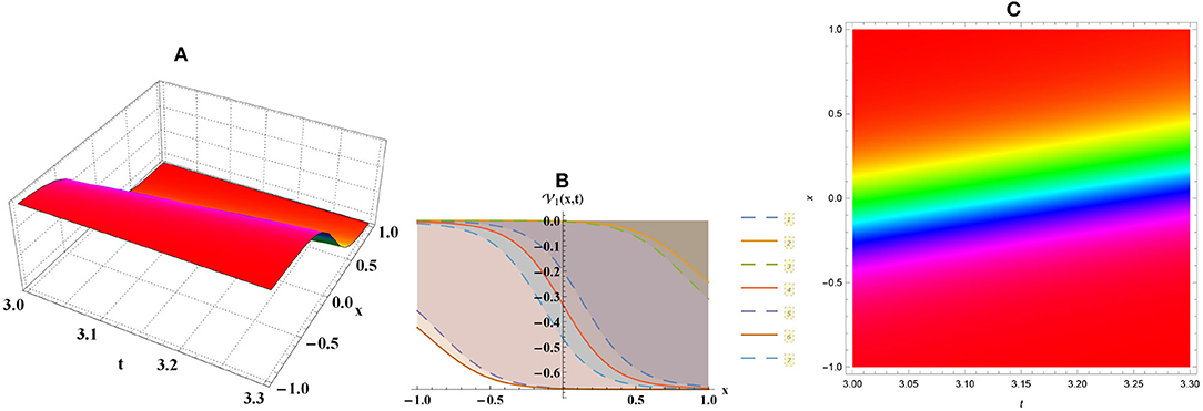
Figure 1. Kink numerical graph for Equation (4) through (A) three-dimensional, (B) two-dimensional, and (C) density plots.

FIGURE 2

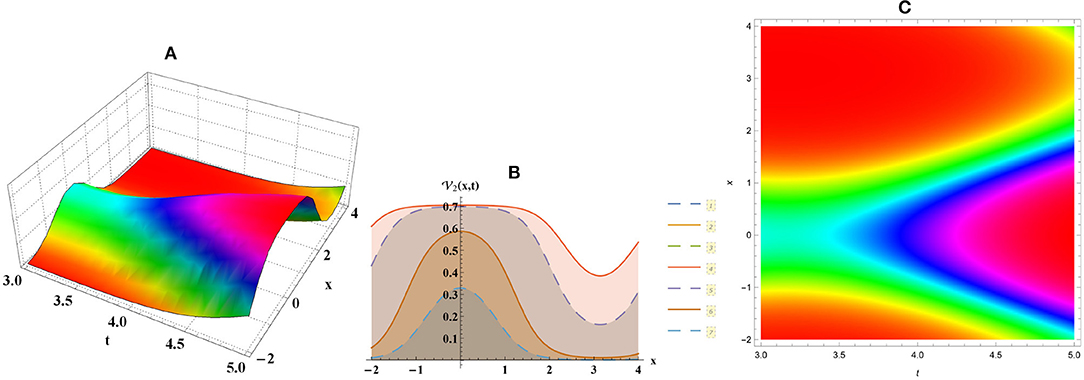
Figure 2. Periodic numerical graph for Equation (6) through (A) three-dimensional, (B) two-dimensional, and (C) density plots.

FIGURE 3

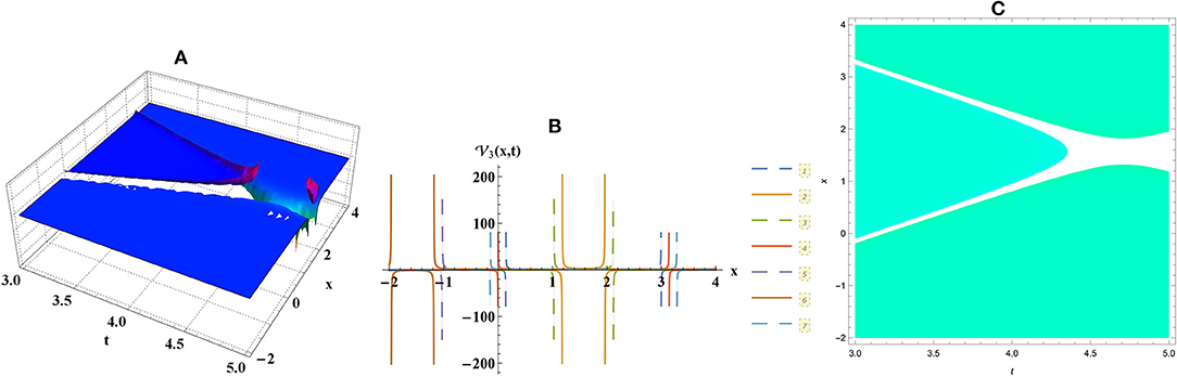
Figure 3. Solitary numerical graph for Equation (7) through (A) three-dimensional, (B) two-dimensional, and (C) density plots.

FIGURE 4

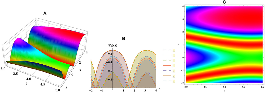
Figure 4. Periodic numerical graph for Equation (8) through (A) three-dimensional, (B) two-dimensional, and (C) density plots.

FIGURE 5

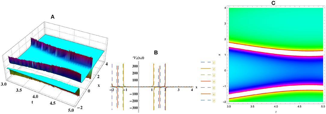
Figure 5. Solitary numerical graph for Equation (9) through (A) three-dimensional, (B) two-dimensional, and (C) density plots.

FIGURE 6

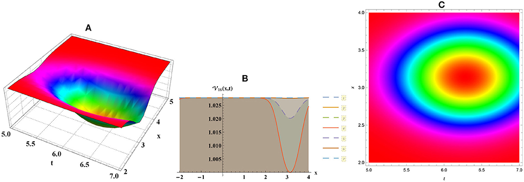
Figure 6. Dark cone numerical graph for Equation (22) through (A) three-dimensional, (B) two-dimensional, and (C) density plots.

FIGURE 7

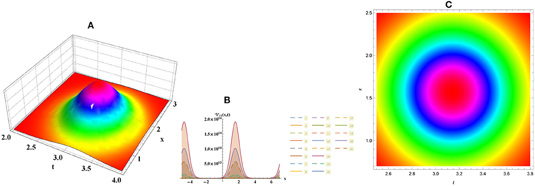
Figure 7. Bright cone numerical graph for Equation (24) through (A) three-dimensional, (B) two-dimensional, and (C) density plots.

4. Conclusion

This study effectively applied three non-applied methods to the FNLTST equation. The compatible fractional operator is used to transform the non-linear fractional partial differential equation into an ordinary differential equation of integer order. Various modern numerical options have been developed to illustrate the cutting-edge or voltage of an electrical transmission spectrum with a day yet distance across two-dimensional, three-dimensional, and density plots. The physical interpretation of these sketches have been explained in Equation (3) to show more novel properties of the considered model. The newness of this study is explored by contrasting the observations in the previous study.

Data Availability Statement

The original contributions presented in the study are included in the article/supplementary material, further inquiries can be directed to the corresponding author/s.

Author Contributions

All authors listed have made a substantial, direct and intellectual contribution to the work, and approved it for publication.

Conflict of Interest

The authors declare that the research was conducted in the absence of any commercial or financial relationships that could be construed as a potential conflict of interest.

Acknowledgments

This research was supported by Taif University Researchers Supporting Project Number (TURSP-2020/48), Taif University, Taif, Saudi Arabia, and the Research Innovation Program for College Graduates of Jiangsu Province (Grant No. KYCX19_1609).

References

1. Khater MM, Inc M, Nisar K, Attia RA. Multi-solitons, lumps, and breath solutions of the water wave propagation with surface tension via four recent computational schemes. Ain Shams Eng J. (2021). doi: 10.1016/j.asej.2020.10.029

CrossRef Full Text | Google Scholar

2. Khater MM, Mohamed MS, Attia RA. On semi analytical and numerical simulations for a mathematical biological model; the time-fractional nonlinear Kolmogorov-Petrovskii-Piskunov (KPP) equation. Chaos Solit Fract. (2021) 144:110676. doi: 10.1016/j.chaos.2021.110676

CrossRef Full Text | Google Scholar

3. Khater MM, Ahmed AES, El-Shorbagy M. Abundant stable computational solutions of Atangana-Baleanu fractional nonlinear HIV-1 infection of CD4+ T-cells of immunodeficiency syndrome. Results Phys. (2021) 22:103890. doi: 10.1016/j.rinp.2021.103890

CrossRef Full Text | Google Scholar

4. Khater MM, Nofal TA, Abu-Zinadah H, Lotayif MS, Lu D. Novel computational and accurate numerical solutions of the modified Benjamin-Bona-Mahony (BBM) equation arising in the optical illusions field. Alexandria Eng J. (2021) 60:1797–806. doi: 10.1016/j.aej.2020.11.028

CrossRef Full Text | Google Scholar

5. Evans DJ, Bulut H. The numerical solution of the telegraph equation by the alternating group explicit (AGE) method. Int J Comput Math. (2003) 80:1289–97. doi: 10.1080/0020716031000112312

CrossRef Full Text | Google Scholar

6. Khater MM, Anwar S, Tariq KU, Mohamed MS. Some optical soliton solutions to the perturbed nonlinear Schrödinger equation by modified Khater method. AIP Adv. (2021) 11:025130. doi: 10.1063/5.0038671

CrossRef Full Text | Google Scholar

7. Khater MM. Novel explicit breath wave and numerical solutions of an Atangana conformable fractional Lotka-Volterra model. Alexandria Eng J. (2021) 60:4735–43. doi: 10.1016/j.aej.2021.03.051

CrossRef Full Text | Google Scholar

8. Khater MM, Seadawy AR, Lu D. Dispersive optical soliton solutions for higher order nonlinear Sasa-Satsuma equation in mono mode fibers via new auxiliary equation method. Superlatt Microstruct. (2018) 113:346–58. doi: 10.1016/j.spmi.2017.11.011

CrossRef Full Text | Google Scholar

9. Khater MM, Nisar KS, Mohamed MS. Numerical investigation for the fractional nonlinear space-time telegraph equation via the trigonometric Quintic B-spline scheme. Math Methods Appl Sci. (2021) 44:4598–606. doi: 10.1002/mma.7052

CrossRef Full Text | Google Scholar

10. Alshahrani B, Yakout H, Khater MM, Abdel-Aty AH, Mahmoud EE, Baleanu D, et al. Accurate novel explicit complex wave solutions of the (2 + 1)-dimensional chiral nonlinear Schrödinger equation. Results Phys. (2021) 23:104019. doi: 10.1016/j.rinp.2021.104019

CrossRef Full Text | Google Scholar

11. Khater MM, Mohamed MS, Elagan S. Diverse accurate computational solutions of the nonlinear Klein-Fock-Gordon equation. Results Phys. (2021) 23:104003. doi: 10.1016/j.rinp.2021.104003

CrossRef Full Text | Google Scholar

12. Khater MM. Diverse solitary and Jacobian solutions in a continually laminated fluid with respect to shear flows through the Ostrovsky equation. Mod Phys Lett B. (2021) 35:2150220. doi: 10.1142/S0217984921502201

CrossRef Full Text | Google Scholar

13. Chu Y, Khater MM, Hamed Y. Diverse novel analytical and semi-analytical wave solutions of the generalized (2 + 1)-dimensional shallow water waves model. AIP Adv. (2021) 11:015223. doi: 10.1063/5.0036261

CrossRef Full Text | Google Scholar

14. Khater MM, Ahmed AES. Strong Langmuir turbulence dynamics through the trigonometric quintic and exponential B-spline schemes. AIMS Math. (2021) 6:5896–908. doi: 10.3934/math.2021349

CrossRef Full Text | Google Scholar

15. Attia RA, Baleanu D, Lu D, Khater MM, Ahmed ES. Computational and numerical simulations for the deoxyribonucleic acid (DNA) model. Discrete Contin Dyn Syst. (2021) doi: 10.3934/dcdss.2021018

CrossRef Full Text | Google Scholar

16. Sun GQ. Mathematical modeling of population dynamics with Allee effect. Nonlin Dyn. (2016) 85:1–12. doi: 10.1007/s11071-016-2671-y

CrossRef Full Text | Google Scholar

17. Lopatiev A, Ivashchenko O, Khudolii O, Pjanylo Y, Chernenko S, Yermakova T. Systemic approach and mathematical modeling in physical education and sports. J Phys Educ Sport. (2017) 17:146–55. Available online at: http://repository.ldufk.edu.ua/handle/34606048/10563

Google Scholar

18. Zhang P, Xiao X, Ma Z. A review of the composite phase change materials: fabrication, characterization, mathematical modeling and application to performance enhancement. Appl Energy. (2016) 165:472–510. doi: 10.1016/j.apenergy.2015.12.043

CrossRef Full Text | Google Scholar

19. Attia RA, Lu D, Ak T, Khater MM. Optical wave solutions of the higher-order nonlinear Schrödinger equation with the non-Kerr nonlinear term via modified Khater method. Mod Phys Lett B. (2020) 34:2050044. doi: 10.1142/S021798492050044X

CrossRef Full Text | Google Scholar

20. Ali AT, Khater MM, Attia RA, Abdel-Aty AH, Lu D. Abundant numerical and analytical solutions of the generalized formula of Hirota-Satsuma coupled KdV system. Chaos Solit Fract. (2020) 131:109473. doi: 10.1016/j.chaos.2019.109473

CrossRef Full Text | Google Scholar

21. Khater MM, Attia RA, Abdel-Aty AH, Abdou M, Eleuch H, Lu D. Analytical and semi-analytical ample solutions of the higher-order nonlinear Schrödinger equation with the non-Kerr nonlinear term. Results Phys. (2020) 16:103000. doi: 10.1016/j.rinp.2020.103000

CrossRef Full Text | Google Scholar

22. Khater MM, Park C, Abdel-Aty AH, Attia RA, Lu D. On new computational and numerical solutions of the modified Zakharov-Kuznetsov equation arising in electrical engineering. Alexandria Eng J. (2020) 59:1099–105. doi: 10.1016/j.aej.2019.12.043

CrossRef Full Text | Google Scholar

23. Park C, Khater MM, Attia RA, Alharbi W, Alodhaibi SS. An explicit plethora of solution for the fractional nonlinear model of the low-pass electrical transmission lines via Atangana-Baleanu derivative operator. Alexandria Eng J. (2020) 59:1205–14. doi: 10.1016/j.aej.2020.01.044

CrossRef Full Text | Google Scholar

24. Khater MM, Alzaidi J, Attia RA, Lu D, et al. Analytical and numerical solutions for the current and voltage model on an electrical transmission line with time and distance. Phys Scripta. (2020) 95:055206. doi: 10.1088/1402-4896/ab61dd

CrossRef Full Text | Google Scholar

25. Khater MM, Attia RA, Baleanu D. Abundant new solutions of the transmission of nerve impulses of an excitable system. Eur Phys J Plus. (2020) 135:1–12. doi: 10.1140/epjp/s13360-020-00261-7

CrossRef Full Text | Google Scholar

26. Li J, Attia RA, Khater MM, Lu D. The new structure of analytical and semi-analytical solutions of the longitudinal plasma wave equation in a magneto-electro-elastic circular rod. Mod Phys Lett B. (2020) 34:2050123. doi: 10.1142/S0217984920501237

CrossRef Full Text | Google Scholar

27. Yue C, Khater MM, Attia RA, Lu D. The plethora of explicit solutions of the fractional KS equation through liquid-gas bubbles mix under the thermodynamic conditions via Atangana-Baleanu derivative operator. Adv Differ Equat. (2020) 2020:1–12. doi: 10.1186/s13662-020-2540-3

CrossRef Full Text | Google Scholar

28. Khater MM, Park C, Lu D, Attia RA. Analytical, semi-analytical, and numerical solutions for the Cahn-Allen equation. Adv Differ Equat. (2020) 2020:1–12. doi: 10.1186/s13662-019-2475-8

CrossRef Full Text | Google Scholar

29. Chen J, Liu F, Anh V. Analytical solution for the time-fractional telegraph equation by the method of separating variables. J Math Anal Appl. (2008) 338:1364–77. doi: 10.1016/j.jmaa.2007.06.023

CrossRef Full Text | Google Scholar

30. Kumar S. A new analytical modelling for fractional telegraph equation via Laplace transform. Appl Math Model. (2014) 38:3154–63. doi: 10.1016/j.apm.2013.11.035

CrossRef Full Text | Google Scholar

31. Orsingher E, Zhao X. The space-fractional telegraph equation and the related fractional telegraph process. Chin Ann Math. (2003) 24:12–45. doi: 10.1142/S0252959903000050

CrossRef Full Text | Google Scholar

32. Guo M, Dong H, Liu J, Yang H. The time-fractional mZK equation for gravity solitary waves and solutions using sech-tanh and radial basic function method. Nonlin Anal Model Control. (2019) 24:1–19. doi: 10.15388/NA.2019.1.1

CrossRef Full Text | Google Scholar

33. Ganji D, Abdollahzadeh M. Exact travelling solutions for the Lax's seventh-order KdV equation by sech method and rational exp-function method. Appl Math Comput. (2008) 206:438–44. doi: 10.1016/j.amc.2008.09.033

CrossRef Full Text | Google Scholar

34. Wang G. A novel (3 + 1)-dimensional sine-Gorden and sinh-Gorden equation: derivation, symmetries and conservation laws. Appl Math Lett. (2020) 113:106768. doi: 10.1016/j.aml.2020.106768

CrossRef Full Text | Google Scholar

35. Kudryashov NA, Loguinova NB. Extended simplest equation method for nonlinear differential equations. Appl Math Comput. (2008) 205:396–402. doi: 10.1016/j.amc.2008.08.019

CrossRef Full Text | Google Scholar

36. Guner O, Bekir A. The Exp-function method for solving nonlinear space-time fractional differential equations in mathematical physics. J Assoc Arab Univ Basic Appl Sci. (2017) 24:277–82. doi: 10.1016/j.jaubas.2016.12.002

CrossRef Full Text | Google Scholar