 Leonhard Lücken
 Sinikka T. Lennartz
 Jule Froehlich
 Bernd Blasius1,3
- 1Institute for Chemistry and Biology of the Marine Environment, Carl von Ossietzky University of Oldenburg, Oldenburg, Germany
- 2Department of Earth, Atmospheric and Planetary Sciences, Massachusetts Institute of Technology, Cambridge, MA, United States
- 3Helmholtz Institute for Functional Marine Biodiversity, Carl von Ossietzky University of Oldenburg, Oldenburg, Germany
A distinguishing feature of many ecological networks in the microbial realm is the diversity of substrates that could potentially serve as energy sources for microbial consumers. The microorganisms are themselves the agents of compound diversification via metabolite excretion or overflow metabolism. It has been suggested that the emerging richness of different substrates is an important condition for the immense biological diversity in microbial ecosystems. In this work, we study how complex cross-feeding networks (CFN) of microbial species may develop from a simple initial community given some elemental evolutionary mechanisms of resource-dependent speciation and extinctions using a network flow model. We report results of several numerical experiments and report an in-depth analysis of the evolutionary dynamics. We find that even in stable environments, the system is subject to persisting turnover, indicating an ongoing co-evolution. Further, we compare the impact of different parameters, such as the ratio of mineralization, as well as the metabolic versatility and variability on the evolving community structure. The results imply that high microbial and molecular diversity is an emergent property of evolution in cross-feeding networks, which affects transformation and accumulation of substrates in natural systems, such as soils and oceans, with potential relevance to biotechnological applications.
1 Introduction
Microorganisms have successfully inhabited both aquatic and terrestrial ecosystems on earth for millions of years, and continuously evolved to an enormous diversity (Pedrós-Alió, 2006; Azam and Malfatti, 2007; van der Heijden et al., 2008; Sunagawa et al., 2015; Thompson et al., 2017). This immense ecological success is related to the observation that microorganisms are able to modify their abiotic environment through the production of organic compounds. Thereby, due to their metabolic activity, microbes act as ecosystem engineers and over the millennia have been able to completely transform and alter the chemical environment on the planetary surface, with drastic consequences for conditions of life and biogeochemical cycles (Falkowski et al., 2008). In the marine environment, for example, microbial transformation of organic compounds is considered to have played an important role in the production of refractory matter, creating a pool of dissolved organic material that resists biodegradation over thousands of years and has accumulated in the oceans to a current reservoir of 700 Petagram carbon—with strong implications for the global climate system (Dittmar and Stubbins, 2014; Dittmar et al., 2015; Dittmar et al., 2021).
Based on their enormous diversity, and mediated by the exchange of metabolites, microbial communities are forming incredibly complex networks of ecological interactions (Lozupone et al., 2012; Nannipieri et al., 2017). In many cases, a substance that a species may or must use for its growth, is excreted by another species as a byproduct, yielding syntrophic or cross-feeding relationships (Hibbing et al., 2010; Morris et al., 2013; Seth and Taga, 2014; Gralka et al., 2020). Recent evidence suggests that such cross-feeding interactions should be a generic feature of microbial ecology (Goldford et al., 2018) and it is believed to be partly responsible for difficulties of cultivating a large portion of microbial species occurring in natural habitats (Tyson and Banfield, 2005). The full importance of cross-feeding for microbial biodiversity is, however, still a matter of debate (Foster and Bell, 2012).
One other defining characteristic of microbial communities is their potential for fast evolution. Due to fast turnover times and the possibility of lateral gene transfer (Jamieson-Lane and Blasius, 2020) new mutations occur frequently even on laboratory time scales (Craig MacLean, 2005). The potential for rapid evolution of metabolic cross-feeding interactions was convincingly demonstrated in a series of long-term experimental studies with microbial populations (Helling et al., 1987; Rosenzweig et al., 1994; Friesen et al., 2004). This was also confirmed in model studies, showing that cross-feeding should naturally emerge if waste products or less valuable compounds are generated during the metabolization of a primary resource (Doebeli, 2002; Pfeiffer and Bonhoeffer, 2004). Additional evidence for naturally occurring rapid evolution of new metabolic pathways comes from observations of microbial degradation of organic pollutants that have been introduced by humans only decades ago (Copley, 2009). For instance, in the marine environment, the increased introduction of plastic waste created a new ecological niche, the “plastisphere”, which serves as colonization habitat for diverse microbial communities, with some of them already having developed enzymatic pathways that can hydrolyze and degrade certain plastic polymers (Sudhakar et al., 2008; Zettler et al., 2013; Paço et al., 2017; Amaral-Zettler et al., 2020).
In diverse microbial communities, such evolutionary inventions will scale up, giving rise to ongoing alteration of metabolic transformations. This dynamic is further complicated by the fact that an altered chemical environment will affect the fitness of individual organisms, leading to extinctions of microbes that have lost essential substrates, while the production of new metabolites provides niches for either speciation or invasion of new microbial consumers—again altering the chemical environment and yielding successive extinction and invasion events. In this way, microbial and molecular diversity mutually sustain each other, in the sense that microorganisms diversify compounds by metabolite excretion and overflow metabolism, and a diverse set of metabolites offers new niches for evolving microbes.
From a theoretical point of view, the resulting closely intertwined dynamics of microbial community structure and the chemical environment can be understood as an adaptive co-evolutionary network. Adaptive networks combine the topological evolution of the network with dynamic changes in the states of the network nodes. They are known to be capable of self-organizing towards critical behavior, spontaneous division of labor, and the formation of complex topologies (Gross and Blasius, 2008) and arise in a large number of areas, including biological and epidemiological systems (Gross et al., 2006). In order to gain an understanding of the resulting complex co-evolutionary dynamics in such systems, theoretic approaches have proven to be a powerful method. One of the most influential conceptual models of large-scale biological co-evolution in this context is a model introduced by Bak and Sneppen (Bak and Sneppen, 1993), which directly assigns a new random value for the fitness of the least fit population and all interacting populations, mimicking the replacement of the former and the alteration of its interactions. Later, Solé and Manrubia proposed a similarly simple model of an ecological network, considering a more continuous drift of properties, and ancestral relations between populations (Solé, 1996; Solé and Manrubia, 1996). Just as the Bak-Sneppen model, it assumes a fixed number of species, but also models the pairwise interactions between species. Nunes Amaral and Meyer (Nunes Amaral and Meyer, 1999) then considered foodweb models and allowed their size and depth to vary, driven by the processes of extinction and speciation.
These conceptual models, based on simple statistical rules, focused on determining the distribution of extinction cascade sizes. They did not, however, allow to simulate the time dependence of consumer, and resource densities. This is possible in another class of models that extend classical consumer-resource models (Tilman, 1982). Besides including resource consumption, models of this class also consider the exudation of compounds by different consumer populations. In turn, these products provide resources available to other populations, which possess metabolic capabilities for consumption. We denote the resulting bipartite network of consumers and resources, in which resource-to-consumer links represent consumption and consumer-to-resource links represent production, as cross-feeding networks (CFN).
The analysis of CFN models received an increasing attention in the past few years (Germerodt et al., 2016; Butler and O’Dwyer, 2018; Goldford et al., 2018; Goyal and Maslov, 2018; Marsland et al., 2019; Mentges et al., 2019; Marsland et al., 2020a; Oña and Kost, 2020). The usual approach for assembling a model community in CFN models is the creation of a meta-population pool, holding the full entirety of existing species. In this step, structural assumptions regarding feasible substrate transformations and consumer traits take effect. Here, energetic and stoichiometric relationships between different compounds or correlations between different metabolic capacities may be considered. This step is then followed by placing a subset of species in a given environment and applying environmental filtering to determine a resulting CFN, which then could represent observed patterns in natural systems (Goldford et al., 2018; Marsland et al., 2019; Mentges et al., 2019; Marsland et al., 2020b).
These studies, however, did not consider evolutionary dynamics. In turn, most of the experimental and modeling studies concerned with the evolutionary emergence of cross-feeding were restricted to situations where only two consumers species interact (Doebeli, 2002; Pfeiffer and Bonhoeffer, 2004; Preussger et al., 2020). An exception is the study of Goyal and Maslov (Goyal and Maslov, 2018), who modeled how a trophic structure involving many, mostly hierarchically organized, consumers can arise from metabolite leakage. In their model, a one-to-one relationship is assumed for consumer species and resources, which restricts the degree of reciprocate interaction in the generated networks. In the progress of the evolution, larger changes become rarer and rarer in the model, as the system develops towards a saturated or optimized state. Besides the work of Goyal and Maslov, the effect of evolutionary processes on complex CFNs has—according to our state of knowledge—not been studied in detail yet.
Given the commonness of CFNs in natural systems (Seth and Taga, 2014), understanding the evolutionary dynamics of CFNs and separating between internal and external variability is crucial. Is the continuous saturation observed in the model of Goyal and Maslov an inherent property of the evolution of CFNs? Or is it a result of the models simplifications, such as the limitation of the trophic dependencies of a consumer to a single resource? In natural environments, microbial consumers thrive on a variety of different substrates, and implying a higher in-degree of the consumer nodes in a network representation than assumed in (Goyal and Maslov, 2018).
In our work, we consider the dynamics of an evolutionary CFN model allowing higher diversities of the consumed and released resources. Without considering the underlying biochemical foundations, we study the emerging network structures, and the time course of their evolution. Our protocol is capable of describing the appearance of novel resources and the corresponding rise of novel metabolic capabilities to exploit these. We report results of several numerical experiments and provide an in-depth analysis of the evolutionary dynamics. Further, we compare the impact of different parameters, such as the assumed metabolic efficiency, versatility, and variability on the evolving community structure. Our findings show that a complex ecological system, which is subject to persisting turnover even in stable environments, can arise from simple assumptions.
The paper is organized as follows. In Section 2, we introduce the model, which comprises a formalism for the calculation of stationary flows in a CFN and a protocol describing the evolutionary development of the network. In Section 3, we provide theoretical results on the maximal system capacity and a numerical analysis of the evolutionary process. In particular, we determine the parameter dependence of stationary flow patterns, as well as structural properties, and biodiversity measures of the evolving system. In the final Section 4, we discuss the relation of our model and its displayed characteristics to previous experimental and modeling studies.
2 Materials and Methods
2.1 Stationary Flow in Cross-Feeding Networks
Cross-feeding networks are directed bipartite networks composed of two different types of nodes: consumers and resources, cf. Figure 1. Thus, two different link types and, correspondingly, two different types of resource flow exist in the network. Links directed from resources to consumers indicate the uptake of a resource by the corresponding consumer, whereas a link from a consumer to a resource describes the release of the resource by the consumer. Deliberately, we do not specify a physical unit for the flow, since the model is generic with respect to different choices thereof. For instance, as a physiological equivalent of the network flow, one may consider moles of carbon transferred from one node to the other, and or being exported to inorganic or accumulating reservoirs. Although we employ this notion of mass flow throughout this work, one could likewise consider the energy bound in the chemical composition of compounds to constitute the unit of measurement (Goyal and Maslov, 2018). We refer to the flow from resources to consumers as “uptake” and to the flow from consumers to resources as “release”. More formally, in a given CFN we denote the set of all resources by
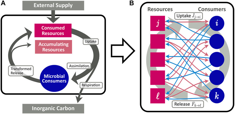
FIGURE 1. Conceptional diagram of the CFN model, describing the flow of organic matter (arrows) between pools of resources (red rectangles), and microbial consumers (blue circles). (A): Aggregated flows between different pools. Organic matter is supplied from an external source to the resource pool. A fraction η of consumed resources is assimilated for microbial growth, while the remainder is lost from the system and remineralized to inorganic carbon. Assimilated resources are eventually recycled and enter the resource pool in transformed molecular composition. (B): Fine grained scheme of the bipartite network of assimilation [red arrows, cf. Eq. 4] and release [blue arrows, cf. Eq. 6].
Besides the release originating in consumers, we allow external supply flows sj at each resource, such that the total inflow rate at resource j is
Our modeling approach assumes a given set of consumers at each moment in evolutionary time. Consumers have specific metabolic profiles, which determine their interaction with the present resources. Each consumer i is equipped with a vector of resource affinities ui,j,
The share
If no consumer exists for a specific substrate at a given time, i.e., ui,j ≡ 0 for all
where
The composition of release by consumer i is assumed to follow the release proportions ϱj,i,
Here, we assume the products to be independent of the composition of the consumption. Combining Eq. 2, Eq. 5, and Eq. 6, we find
Or in vector, resp. matrix, notation:
with vectors
Solving for F yields
Since the mapping T represents merely a redistribution of the flow across the resource network, it will never increase the total flow, i.e.,
for all v ≥ 0, where
Thus, the internally generated network flow is obtained by the iterative transport of the supply flow through the network. Note the formal relationship of Eq. 7 to the definition of the weighted Katz centrality (Katz, 1953; Newman, 2010) associated with the resource transformation matrix T. This has a simple interpretation: the stationary resource flow through consumer i is proportional to the weighted sum of flows through the network neighbors of i plus the input flow from the external source.
2.2 Evolutionary Generation of Cross-Feeding Networks
While in the previous section we determined the stationary resource flow for a given CFN, we now define the rules that lead to evolutionary changes in the CFN. In our protocol, the change of the CFN within one evolutionary time step is determined by two stages: 1) The randomized generation of a new consumer species with an ancestor in the resident community, and 2) the calculation of the impact of its introduction on the CFN, including eventual extinctions and a modification of the network flow pattern.
The procedure assumes that the evolutionary time scale, where adaptations of the metabolic capabilities and introductions of new consumer species occur, is separated from the timescale of ecological processes that lead to an equilibration of the network flow. Furthermore, we avoid the calculation of population densities and resource concentrations by describing the system exclusively by the network flow.
In the first stage, a new consumer species i is introduced into the community. It is assigned an ancestor a in the resident community, which is chosen at random, but with a probability weight proportional to Ja. The descendant k’s characteristics are then altered on the basis of the ancestor’s. More precisely, given the affinities ua,j and release fractions ϱj,a of the ancestor, the corresponding characteristics of the descendant are set proportional to
where ɛj,1 and δj,1 are independently, uniformly distributed in
and
with random variables ɛ* and δ* drawn from a uniform distribution
Limiting the total affinity may be considered to represent the limited investment each consumer may place on transporter enzymes and other metabolic machinery associated with the utilized resources (Posfai et al., 2017; Mentges et al., 2019).
A second possible substep of the first stage, is executed with a probability pu. Here, we allow for a qualitative change of the new consumer’s metabolism by substituting one utilized resource j, i.e. ui,j > 0, for another j′ with ui,j′ = 0. That is, after the substitution resource j′ takes the affinity formerly assigned to j, resulting in ui,j = 0 and ui,j′ > 0. In contrast to the gradual changes of affinities and release fractions in Eq. 11, this qualitative adjustment of metabolism mimics a mutation allowing the species to exploit a novel resource. Similarly, with a probability pϱ, we alter the release configuration to substitute an old product for a new one, drawn at random from a global resource pool
In the second stage of an evolutionary time step, we add the newly generated consumer species to the resident community
the species with lowest Ji below μ is considered extinct and is removed from
Figure 2 illustrates an evolving CFN at different steps in evolutionary time. It is obtained from the stepwise evolution starting at a single species at t = 1 up to N = 95 species at t = 400. The evolutionary algorithm operates with parameters nu = nϱ = 3 and pu = pϱ = 0.2, and a single resource is externally supplied. Note that the single founding consumer species (blue dot in the leftmost graph) is also capable to consume nu = 3 different resources, although only one supplied resource is present and depicted, initially. In the subsequent steps, additional consumers are generated. As metabolic novelties evolve, new compounds (red squares) are released and metabolized by the growing community. Clusters of consumer nodes can be observed, which share similar metabolic properties. In Section 3.4, we study the clustering in more depth.
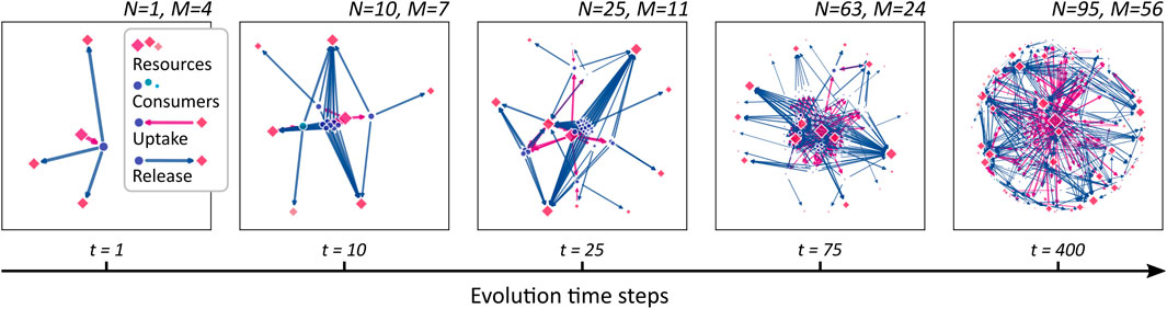
FIGURE 2. A growing cross-feeding network. Starting from a founding consumer (leftmost panel), new consumers (blue dots) are added sequentially leading to an increasing community size N. As novel metabolic capacities evolve, the number M of different resources (red squares) increases. The symbol sizes are scaled proportional to the stationary flow passing through the corresponding network node. Uptake links are drawn as magenta arrows, release links as blue.
3 Results
3.1 Theoretical System Capacity and Total Flow
Due to respiration losses and the finite external supply rate, the number of consumers, which can be sustained in the CFN model, is finite. To determine an upper bound for the number of consumers, let us consider the total flow rate
Then, (9) implies
Note that by definition
If all resources were consumed, an additional flow of ηA would enter the system via the consumption of the accumulating resources and generate an amount
of additional flow until its complete respiration. Taking this into account, we can state more precisely:
By definition, the total uptake flow
Because a consumer population is only considered persistent if Eq. 12 holds, the total number of consumers cannot exceed
where
3.2 Simulation Results
In the following, we consider the simulation of the evolution of a CFN according to the protocol defined in Section 2 with parameters as defined in the caption of Figure 3. We assume that the external supply enters the pool of resource j = 0 at a fixed rate s0 ≡ 1.0, mimicking a static environment, which allows us to study the internal dynamics of the CFN. Panels A–F of that figure show the evolution of several measures for an evolving CFN initialized with a random founding species, which has positive affinities for the supplied substrate (and two other substrates not present at the beginning of the simulation). Its release diversity is set to nϱ = 3 and is inherited to all its descendants. The time series are split up into a magnified view of the initial phase and a larger, later interval when the system exhibits statistically stationary fluctuations.
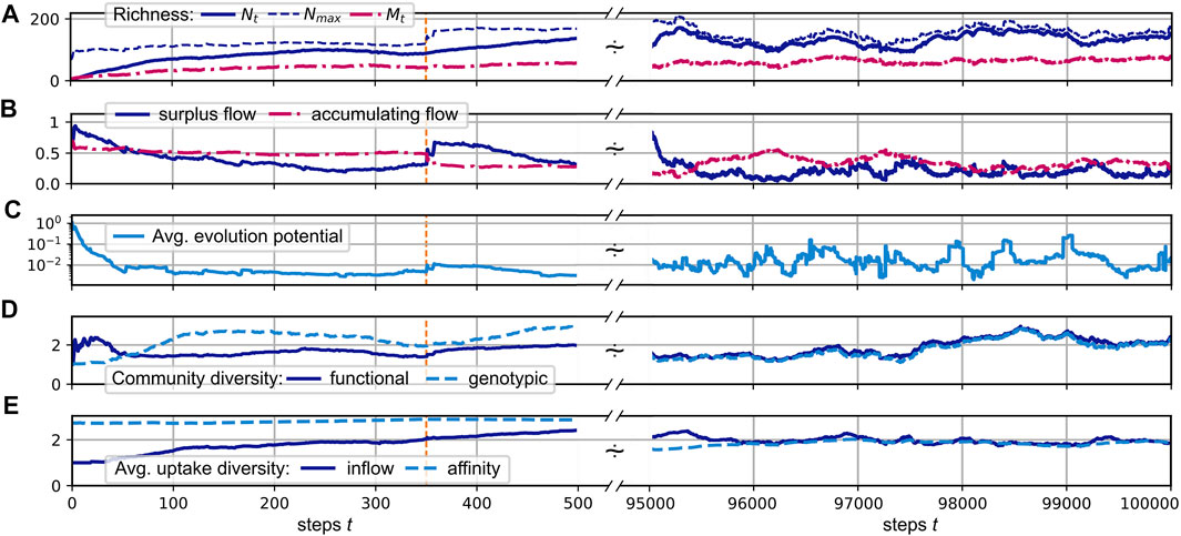
FIGURE 3. (A–E): Different community measures over the course of a simulated evolution. The initial time interval of steps 0 to 500 is magnified, with a dashed orange vertical line indicating step 350. An interval [500, 9.5 × 10⁴] is skipped and the interval [9.5, 10] × 104 is displayed at the right side. See the main text for the definition of the shown quantities. System parameters are nu = nϱ = 3, η = 0.7, μ = 0.01, pu = pϱ = 0.2, α = 0.2,
3.2.1 Richness
Panel A of Figure 3 illustrates the development of the consumer and substrate richness,
3.2.2 Network Flow
As shown in Panel A, the realized richness remains below the upper limit Nmax. This implies that either the uptake rates of some consumers significantly exceed the subsistence flow, i.e., Ji ≥ μ, or some of the network flow leaks out of the system into resources, which are not consumed, i.e., A > 0. Panel B shows that both is the case, in general. Neither does the accumulation flow A drop to zero, nor does the “surplus flow”
3.2.3 Evolutionary Potential
The fraction of flow into accumulating resources represents a measure for the potential of novel metabolic capabilities to allocate additional resource flow for their bearer. Further, the fraction of surplus flow corresponds to the fraction of flow which can be consumed by additional consumers without inducing a displacement of present consumers. However, if the surplus flow of a specific consumer i falls towards zero, it faces the risk of being displaced by another consumer, which has a superior combination of affinities. Any offspring k, whose affinities would increase the uptake in comparison to consumer i has the potential to do so. Let us assume the substitution of consumer i by a similar consumer k. Ignoring nonlinear effects and impacts from changing network flow patterns, a first-order estimate can be given for the total uptake flow Jk acquired by consumer k in terms of the affinity differences δj≔uk,j − ui,j, by
Thus, to measure the potential for increasing the fitness of consumer i, one may consider the redistribution of its affinities ui,j which maximizes Eq. 18. Recall, that the admissible variation of the affinities is constrained to preserve the total affinity
We call ΔJi the “evolutionary potential” of consumer i and we report its average over the whole ensemble
A straightforward calculation shows that
where the value Rj = Fj/∑nun,j.
The convergence of ΔJi to zero would indicate an evolution towards an optimal, saturated system state where the present ensemble of consumers can hardly be invaded. However, in our simulations, it fluctuates around finite values, indicating an ongoing co-evolution, which constantly creates new niches, and results in a persistent community turnover with time. Thus, despite a constant supply flow, the system does not reach an evolutionary stable community.
3.2.4 Diversity
Figure 3D in Figure 3 shows measures for the genotypic and functional diversity of the consumer community. We calculate these diversity indices based on the pairwise species similarities zi,k,
The diversity D for the whole community is calculated as the inverse of the average ordinarity, i.e.,
We note that 21 corresponds to the diversity of order q = 2 as defined by Leinster and Cobbold (Leinster and Cobbold, 2012).
In the simulation run shown in Figure 3, both diversity measures fluctuate relatively synchronously around an average value of about 2.1. This relatively low value, compared to the average consumer richness of about 125 (see Figure 3A), can be explained by the fact that a large cluster of consumers concentrates its efforts on the consumption of the only supplied resource j = 0, which has the highest inflow of F0 ≳ 1.0, and a few produced resources, which have higher availability. On average, two thirds of the consumers exhibit an uptake flow, which is composed to more than one half from the supplied resource. See also Figure 4A, which describes the relationship of evolved affinities and substrate flows, and is discussed below.
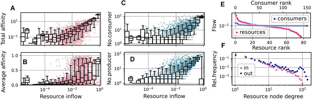
FIGURE 4. Community and network statistics for the simulation run shown in Figure 3, taking into account steps t ≥ 50000. (A–D): Resource flows
Figure 3E shows the evolution of the average uptake diversity of individual consumers. As a measure of consumer i’s position on a range from being a single resource specialist or a generalist, we calculate the effective richness (Leinster and Cobbold, 2012)
of its relative affinities
The relation of the total effort dedicated to the competition for a resource and its availability is illustrated by the statistics shown in Figure 4A. Here, each red dot shows the relation of the total affinity
to the stationary flow Fj for a specific resource j at a specific time step t from a sequence of community states
The overlaying boxplot summarizes the distribution of points for the corresponding bins, indicating the median and the 25–75% quantile range within the box and the 5–95% range within the whiskers. A linear regression to the double log data restricted to resources with Fj > 0.001, yields an exponent
Similarly, as visible in Figures 4C,D, the number of consumers increases with the availability of the resource, and the availability of a resource increases with the number of associated producers. For the latter relation, the supplied resource forms an exception, as its inflow is high without necessarily having a large number of producers.
In Figure 4B, we show the distribution of the average affinities of consumers over specific resources. We observe an interesting pattern of transition from high to low average affinities depending on the resource flows Fj. For the supplied resource the average affinity is close to one, indicating specialist consumers. On the other hand, for resources with low inflow, we observe mainly low affinities. In the mid range, though, substrates may bear both, specialists and generalists.
In Figure 4F we show the distributions of logarithmic in-degrees and out-degrees of the resources node, i.e., of the number of consumers and producers associated with present resources. Here, we observe an approximate power law scaling of relative frequencies with exponents ≈ − 1.28 (for in-degrees) and ≈ − 1.08 (for out-degrees) up to degrees
Figure 4E shows an exemplary diagram of rank vs stationary flow in the last community
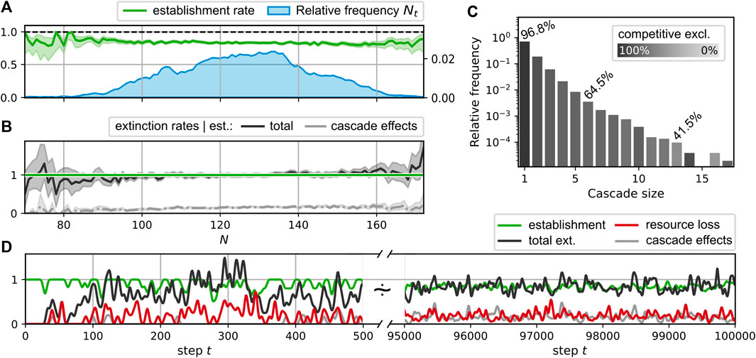
FIGURE 5. Displacement statistics for the simulation run shown in Figure 3; (A–C) take into account steps t ≥ 50000. (A): Average success rate for the establishment of the new consumer generated in a step t given the community size Nt (green curve); observed distribution of Nt (blue curve). (B): Average rate of extinctions given a successful establishment of a new species in dependence of the community size Nt. Black curve: total extinction rate; gray curve: extinctions due to cascade effects. Shaded regions around the average rate curves represent central 95% credibility intervals [beta distribution for establishments in A, gamma distribution for extinctions in B]. (C): Extinction cascade size distribution. Each bar represents the relative frequency for extinction cascades of the corresponding size; the lightness level is determined by the percentage of extinctions due to cascade effects, i.e., non-competitive interactions. Exemplary values for these percentages are stated explicitly. (D): Smoothed time series of consumer establishments (green), extinctions (black), the corresponding subset of non-competitive exclusions (gray), and the loss rate of resources (red). Smoothing was performed with a Blackman window (size 15 for t ∈ [0, 500], size 100 for t ∈ [9.5, 10] × 104) as described in Ref. (SciPy contributors, 2017).
3.3.5 Displacement
During the simulation run shown in Figure 3, the consumer richness saturates after an initial growth phase of the network and fluctuates around finite values of Nt ≈ 125 < Nmax, where
For the observed extinction events, we may differentiate between two types of extinctions. Firstly, we classify events as competitive exclusion if the extinct consumer is a direct competitor to the newly introduced consumer, i.e., extinct and new consumer share at least one resource. Secondly, there are indirect effects, which may cause extinctions by the altered resource flow pattern at a different network location. For instance, reduced resource flows may result due to extinctions or increased competition for their producers. We call the category of the latter phenomena “cascade effects”. Figures 5B and D differentiate between these two cases, showing the fraction of extinctions attributed to cascade effects as lighter gray curves. The total fraction of extinctions attributed to cascade effects in this sense is about 14.8%. It is larger for steps where more than one consumer goes extinct. The distribution of the extinction cascade sizes is shown in Figure 5C. Here, the corresponding bars are shaded by the fraction of extinctions attributable to the direct competition with the new consumer. For comparison, these fractions are annotated for selected bars. Fitting an exponential distribution, we obtain a decay of cascade size frequencies with an exponent of −0.27.
3.3 Parameter Sensitivity
In this section, we assess the effect of a number of selected parameters on the evolution of the CFN. Figure 6 shows various measures for an array of numerical simulation experiments with specific parameter sets. Each row contains information about four different experiments, which implement a gradient for the value of a specific parameter, see legend on the left. All other parameters were fixed to the values stated in the caption of Figure 3. The reported quantities are averaged over the step interval
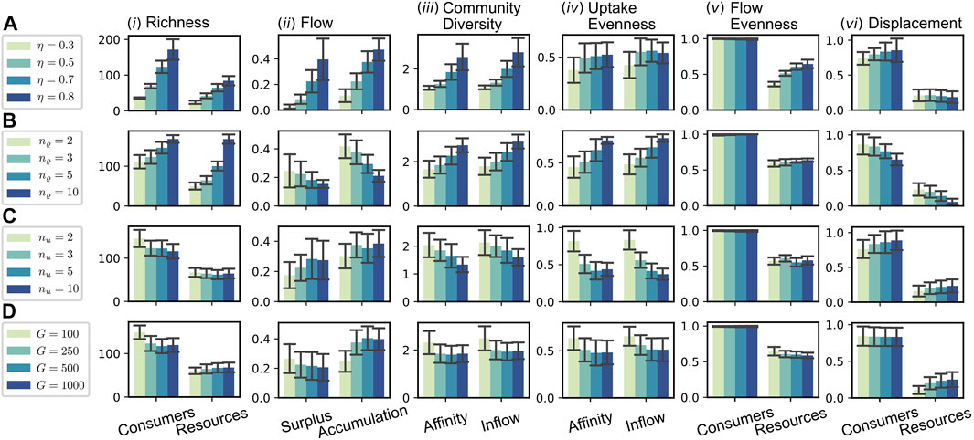
FIGURE 6. Parameter dependence of macroscopic measures. The rows (A–D) each refer to the variation of a particular parameter [(A): recycling fraction η; (B) release diversity nϱ; (C) uptake diversity nu; (D) global resource pool size
3.3.1 Variation of the Recycling Fraction η
In the first sequence, cf. Figure 6A, we tested four different values for the recycling fraction η, ranging from 0.3 to 0.8. Recall that the flow scales with
3.3.2 Variation of the Release Diversity nϱ
Similar as for the sequence A of varying recycling fraction η, we find an increase in consumer and resource richness for higher values of nϱ in sequence B. In contrast to A this increase is more pronounced in the resource richness. The latter seems intuitive: as each consumer produces a higher number of resources, the total pool of resources grows. That this leads to a higher consumer richness, seems to be a consequence of a specific flow pattern, different to the one in case A. While the consumer richness increases [see Figure 6B (i)], the flow per consumer decreases and likewise does the fraction of flow into accumulating resources [see Figure 6B (ii)]. Thus, a higher percentage of the flow is assimilated and more equally distributed among consumers for higher values of nϱ. The reason for this more efficient exploitation of the system’s resources seems to be the increased stability resulting from the fact that produced resources tend to be formed by more different producers. Therefore, a single species’ extinction is less severely affecting the environmental conditions, allowing the evolutionary adaptation to keep the pace of environmental change. This stability is also reflected in the significantly reduced extinction rates for higher nϱ [see Figure 6B (vi)] and a decreased average evolutionary potential (by a factor of
3.3.3 Variation of the Uptake Diversity nu
Regarding sequence C of Figure 6, one might expect, that an increase of the uptake diversity nu would have similarly stabilizing consequences as an increased release diversity nϱ (see case B), since a consumer could now be able to hedge its necessities across a higher diversity of compounds. However, in contrast to case B, the consumer richness decreases, while the average extinction rate slightly increases. A difference between the parameters nϱ and nu is that nu controls the dimension of the parameter space’s portion most directly relevant to the consumer fitness, i.e., the value of its uptake flow Ji. Thus, we conjecture that this is a potential source for the increased instability of systems with increased uptake diversity nu. Since the exploration of the affinity parameter space is more difficult, this decreases the pace of evolutionary adaptation. At the same time, the impact on environmental conditions per extinction is, insofar it is controlled by nϱ, the same in all considered scenarios of sequence C. Indeed, the mean value of the average evolutionary potential Eq. 19 is maximal for the case nu = 10 among all considered simulations and about 5-fold as high as the value in the reference case nu = 3 displayed in Figure 3.
3.3.4 Variation of the Global Resource Pool Size G
In Figure 6D, we have varied the size
3.4 Cluster Dynamics
In our framework, consumers may be more or less similar, or even identical, to each other, and if compared on the level of their metabolic characteristics. To characterize and compare the structure within different communities and its change over time, we pursue an approach based on ancestral relations and similarity clustering of consumers. A cluster in our context may be considered to correspond to a taxonomic unit consisting of different variants or closely related strains of a common taxon.
Based on such an approach, we obtain a representation of evolutionary change as shown in Figure 7 for different parameter sets. Every node in the diagram represents a cluster of similar consumers at a corresponding step in evolutionary time. A link between two clusters at subsequent time points is postulated if an ancestral relationship between these clusters exists. We start with an initial hierarchical clustering of a community at a given initial step t0. The dendrograms on the left of each timeline show this initial clustering, which does not take into account any ancestral information. The subsequent development of clusters through time is defined as follows. If a new consumer establishes itself in the community, it is added to the cluster its direct ancestor belongs to. However, if the diameter of the extended cluster exceeds a specified threshold ϑ, it is split into two, assigning a slightly altered color to the part containing the new consumer. For the initial, as well as for the separative, clustering, we use a hierarchical approach (Virtanen et al., 2020) based on the pairwise “genotypic” dissimilarity of two consumers defined as
for any pair
Figures 7A–D shows four representative cases of community dynamics with different features for the step interval
where AΔB denotes the symmetric difference of A and B. Panels G and H show the densities of the logarithms of the cluster sizes (in G) and of the cluster lifespans (in H). The latter are computed as the number of steps between a cluster’s first appearance and its disappearance when its last member goes extinct.
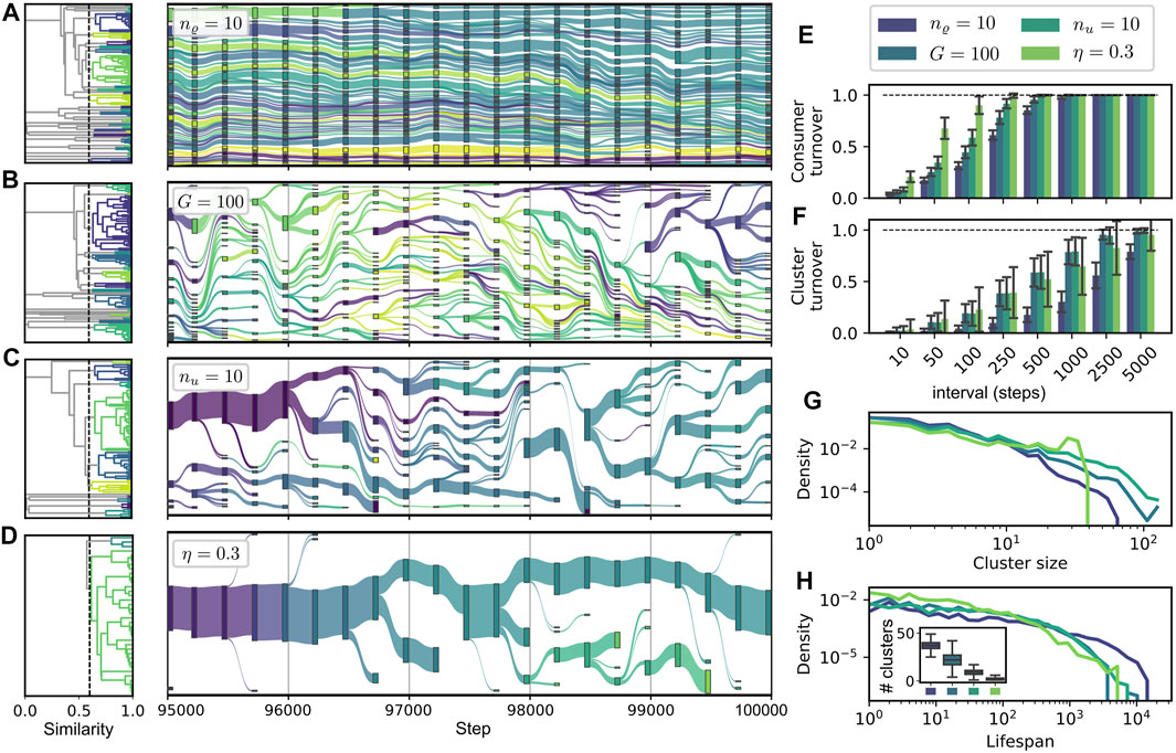
FIGURE 7. Dynamics of similarity clusters of consumers. (A–D): alluvial diagrams of cluster lineages. The link weights between two ancestrally related clusters at steps t and t + 1 are computed proportional to the relative size of the cluster at step t + 1. Dendrograms to the left show the initial clustering of the community at step t = 95 000 used as a basis for the remaining evolutionary tree. We use parameters ϑ = 0.4, wu = 1.0, wϱ = 0.2 (see main text); other parameters as in Figure 3 or indicated in the legend. Visualization with plotly (Plotly Technologies Inc., 2015). (E, F): Average turnover statistics comparing communities
Figure 7A displays a case of high diversity and high stability, corresponding to the parameter variation of high release diversity nϱ = 10, which is also reported in Figure 6 as part of the sequence B. For this case, the turnover on consumer level as well as on cluster level is the lowest among all depicted cases (cf. Figure 7E,F), while the average lifespan of clusters is the highest, cf. H. Due to their relatively high number, the individual clusters are smaller than in most other cases, cf. G and H.
Cases B and C correspond to the parameter variations of small global resource pool size G = 100 and of high uptake diversity nu = 10. Both cases exhibit intermediate turnover rates on consumer and cluster level, which can be associated with the intermediate consumer displacement rates reported in Figure 6C (vi), B (vi) for both cases. Interestingly, we see a higher consumer turnover for nu = 10, while the cluster turnover is approximately equal for both cases. At first glance, one might think that the decreased resource pool turnover for the case G = 100 [cf. Figure 6D (vi)] could stabilize the environmental conditions, allowing for a more gradual shift in the community composition. Such gradual shifts would correspond to more constant clusters, because a cluster could gradually follow the environmental shift without splitting up. On the contrary to these considerations, we find a relative decrease of the cluster turnover for nu = 10, i.e., the ratio of cluster turnover to consumer turnover is smaller for this parameter variation. Note that the case G = 100 exhibits a higher richness and diversity [see Figure 6D(i), D(iii)], and on average more clusters [cf. Panels B and G], which might be responsible for relative increase in the cluster turnover.
An even smaller ratio of cluster to consumer turnover [cf. Panels E and F] is displayed by the parameter variation η = 0.3, where we find the highest consumer turnover rates, while the cluster turnover, especially for longer time intervals, is even lower than for the cases B and C. The distinguishing characteristic of the cluster structure for the case η = 0.3 is the concentration of almost all consumers in a single, large and stable cluster, which leaves its trace in the cluster size distribution as a bump around a value of 120, see Panel G. This low cluster diversity emerges from the low diversity of resources and consumers for low recycling fractions η—cf. Figure 6A and the corresponding discussion in Section 3.3. Due to the scarcity of different niches, only a few branchings from the main cluster of supply consumers take place. Smaller clusters disappear in the majority of cases, indicating a gradual evolution rather than large innovative steps.
4 Discussion
4.1 Model Assumptions and Limitations
Several idealizations or simplifications were assumed in the derivation of the model. Perhaps, the crudest simplification may seem to be the limitation of the number of different organic compounds to a maximal global resource pool size G, which lies orders of magnitude below the number observed in natural systems. For instance, the oceanic DOM was estimated to be composed of more than 100, 000 different compounds (Zark and Dittmar, 2018). However, the effect of larger resource pool sizes in our model is that the probability for each newly evolved release substrate to be already present in the system tends to zero. Apparently, this limit is already well approximated by a resource pool of size G = 500 in our setup, which does not lead to significantly distinct behavior compared to G = 1,000, cf. Figure 4D. The size, where an increase of G does not lead to significantly different evolutionary dynamics, may increase with the number of consumers and the diversity nϱ of released resources per consumer species, but whether this could lead to qualitative differences in parameter dependencies is questionable.
As another simplification, we assumed no particular properties for any of the resources aside of the designation of a supply point. No preferential attachment or evolutionary drive towards the most abundant resources was assumed beyond that. Further, each resource had the same nutritional value for each consumer. Indeed, neither the assimilation efficiency was varied, i.e., ηi,j ≡ η, nor was the total affinity
The most important characteristic displayed by the model, i.e., the ongoing co-evolution, is not affected by the above simplifications, because the fundamental mechanism, driving the continuous turnover of the presented CFN, and does not rely on any of these simplifications. This mechanism is the appearance and disappearance of produced metabolites, which is subject to an undirected evolutionary drift, that constantly alters the environmental restrictions of its beneficiaries, i.e., consumers living on that products. The drift of release configuration is undirected, because the producer’s own fitness, that is its associated inflow Ji, is largely independent of the exact configuration of its products.
The evolutionary dynamics displayed in our model do not stably reproduce all types of resource-mediated ecological relationships. For instance, there is no stabilizing mechanism for reciprocal cross-feeding, which is frequently observed in microbial communities (Morris et al., 2013; Seth and Taga, 2014; Preussger et al., 2020). To see that, consider the simple scenario of a pair of consumers i and k, consuming each other’s products. In this situation any consumer i′ with affinities leading to a total uptake of Ji’ > Ji has the potential to displace consumer i, even if it does not produce any of the resources consumed by k. This is a variant of the tragedy of the commons (Hardin, 1968), since each produced resource in our model is in principle accessible to each consumer. The development of stable reciprocal cross-feeding in natural microbial communities is believed to be a stepwise process (D'Souza et al., 2018; Preussger et al., 2020). The first step is an accidental bidirectional exploitation of metabolic waste products as it also may arise in our model. However, the stabilization and optimization of the syntrophic relationship involves processes beyond the scope of our model. For instance, a spatial association may stabilize a pair of cooperative strains as has been demonstrated recently (Germerodt et al., 2016; Pande et al., 2016). Under which circumstances such a stabilization could counteract the perpetual turnover exhibited by our model is not obvious and could be a subject for further studies.
A distinctive feature of our model is that we assume fixed resource affinities for the different consumers. That is, we do not explicitly model a variable population density for each consumer, but instead simply account for its presence or absence by comparing total uptake against a threshold value μ, cf. Eq. 12. In a usual population dynamic model, resource uptake would be variable, increasing with the consumer’s densities. The parameter μ would take the role of a mortality rate and the difference Ji − μ would describe the instantaneous per capita growth rate of the corresponding consumer. In that framework Eq. 12 would result in a negative growth rate, potentially leading to extinction of the consumer. Our model is, however, able to ‘mimic’ such variable population densities, since consumers tend to produce similar descendants and thus, a cluster of similar consumers quickly populates any available resource. Translating a cluster into a framework of variable population densities, it corresponds to a population with an internal variability. Although the quantized representation of population densities is a simplification with respect to continuous representations, it reflects the intraspecific variation inherent to the concept of a taxonomic unit (Sokal and Sneath, 1963).
4.2 Resource Diversification and Community Turnover
Our CFN self-organizes towards a high level of diversity in both substrates and microorganisms, even after starting with a single microorganism in the in silico experiment. Diversification in our model occurs in two aspects, which are both in line with empirical evidence: first, microorganisms transform and release compounds that can serve as substrates for other microorganisms (i.e., they diversify compounds) and second, a diverse set of compounds in turn can support a diverse microbial community. Indeed, the exometabolome of heterotrophic microorganisms shows a remarkable diversity, even when grown on a single substrate (Ogawa et al., 2001; Wienhausen et al., 2017; Noriega-Ortega et al., 2019), providing potential new niches for other microorganisms. In this context, the role of enzyme promiscuity has been highlighted as a possible mechanism to potentiate the number of transformed resources and has been suggested to contribute to the huge diversity of organic compounds dissolved in seawater (Dittmar et al., 2021). This ability of enzymes to produce new, promiscuous products and to work on substrates besides their canonical substrate spectrum, may trigger the evolutionary development of new metabolic pathways (Tawfik and Tawfik, 2010). Evolutionary diversification of substrate associations has been observed in a laboratory experiment, in which E. coli was grown on glucose as a single substrate under static environmental conditions. After more than 400 generations, strains evolved that did not primarily depend on glucose anymore but rather on metabolites exuded from E. coli (Helling et al., 1987; Craig MacLean, 2005). Furthermore, compared to evolution of isolated strains, bacteria seem to evolve even more rapidly when interacting with other species (Lawrence et al., 2012). Our results corroborate the hypothesis that this high diversity of substrates and microorganisms is self-sustaining and a direct result of cross-feeding interactions subject to evolutionary dynamics.
While the high level of diversity remains fairly constant, the actual microbial and molecular community is constantly turned over. This process is fueled by the recurrent interaction of consumers and resources. With each appearance or disappearance of a new substrate, the fitness of individual microorganisms is modified, leading to changes in the consumer community. On the other hand, each establishment of a new species impacts the composition of available substrates. Experimentally, microbial selection and community assembly has mainly been studied with regard to changing environmental conditions. Only few studies specifically targeted microbial community turnover at stable conditions. In line with our results, a continuous turnover under static conditions has been directly or indirectly suggested: Danczak et al. (2018) found an uncoupling between environment and the development of microbial communities in unperturbed aquifers, leading them to hypothesize that unperturbed environments house dynamic communities due to external and internal forces. Similarly, Konopka et al. (2015) concluded that probably no natural microbial community truly reaches steady-state, but rather exists in a constant flux, which is in line with a metaanalysis by Shade et al. (2013). Our results suggest that an ongoing evolution of syntrophic or commensal interactions is a potential internal mechanism, contributing to the observed constant turnover of microbial community composition.
4.3 Microbial Community Structure
Despite the constant turnover, the community composition in our simulation experiments shows the emergence of specialist and generalist consumers. Here, a microorganism in the network is considered a generalist if the uptake is distributed evenly among different substrates, whereas specialists mainly rely on a single resource. Although our model is deliberately set in a static environment, we observe both strategies non-randomly distributed in the network. Specialists occur in network locations around a less diverse but highly concentrated inflow, i.e., at the constantly externally supplied resource, cf. Figure 4B. On the other hand, resources within the diet of a generalist usually exhibit significantly lower inflows, and fluctuate stronger when new species establish. These fluctuations result from the evolutionary drift of the composition of released resources, which do not directly affect the realized fitness of a consumer. The slow, constrained evolution of affinities, which optimizes a sub-community on a persistently supplied resource, is accompanied by an unconstrained, rather rapidly drifting combination of products that are formed from the metabolization of the more persistent resource. In line with our simulations, the experimental evolution of a bacterium (Pseudomonas fluorescens) showed that in complex environments with many substrates, neither narrow specialists nor complete generalists evolve but rather overlapping imperfect generalists, which have adapted not to all but a certain range of substrates (Barrett et al., 2005). Several examples of heterogeneous microbial communities seem to show strategies of evolving to optimize bet-hedging for substrates (Beaumont et al., 2009; Grimbergen et al., 2015; Haaland et al., 2019). Observations from stability patterns in wastewater treatment plants show dynamics similar to the emergence of characteristic patterns resulting from differences in the resource flows in our model (Werner et al., 2011). Our results indicate that these patterns may already emerge from the basic principles of diversification and evolution that our idealized CFN model is set on. A more decisive exploration of the relation between fluctuation of abiotic factors and evolving patterns of resource specialization in CFNs represents an interesting subject to further research.
Additionally, microbial networks often show a clustered topology, as was shown, for example, in soils (Barberán et al., 2012) or oceans (Cram et al., 2015). This is reminiscent to the clusters observed in our and other author’s models. For instance, Goyal and Maslov (Goyal and Maslov, 2018) reported that their model is capable of reproducing a structure of a core community, containing species of high abundance, combined with peripheral, less abundant species. For a range of parameter values, such patterns are reproduced in our model; they correspond to unequal cluster sizes, which follow the magnitude of flow associated with the utilized resource pools (most apparent in Figure 7D). In addition to the results presented in (Goyal and Maslov, 2018), we found more diverse network structures depending on the system parameters. Thereby, our numerical simulations indicate that the diversity of released resources nϱ, and the fraction of recycled flow η are the most significant factors for the structure of the resulting communities.
It is worth noting that our—as well as Goyal and Maslov’s—results do not rely on any inherent biochemical nature of the different resources. Although the magnitude and diversity of the externally supplied resource flow influences the complexity of a resident community, in our model a complex community emerges from a single, basal resource that is externally supplied. One may ask: how much of the structure of natural communities is emergent, and how much is an artifact of an underlying restriction of resource transformations or, more general, of the constraints of the chemical Universe? The molecular space possesses a wealth of molecular structures, and microbial metabolism is subject to chemical constraints such as elemental stoichiometry of uptake and release, energetic gains during heterotrophic metabolic transformations or preferences of macromolecules such as sugars, lipids or amino acids (Marsland et al., 2020b). These constraints define possible combinations of uptake and release configurations (Goldford et al., 2018; Marsland et al., 2019). As our results show that a structured CFN may develop without such assumptions, we conclude that the degree of correlation between resource availability with respect to the abovementioned constraints, and the community of microbial consumers is not necessarily high. Thus, a quantification of the emergent fraction in community composition represents an important matter of further research.
In summary, we studied a model for the evolutionary change of CFNs and presented a numerical analysis of the influence of several parameters on emerging structural properties. Our model provides a framework to study natural evolutionary and radiation processes in microbial ecosystems and shows that, when combined, these do not lead to a stable microbial community but rather to a persistent co-evolution and turnover, even when environmental conditions remain static. We showed that, starting from one microbial consumer feeding on a single substrate, CFNs can self-organize into systems with diverse, coexisting microorganisms producing, and feeding on numerous substrates. The diversity of the system is self-sustaining because new microbes produce new substrates, which in turn allow for the establishments of new microbes. While the community is constantly turned over, the diversity of compounds and microbes eventually saturates, where the asymptotic diversity of resources depends strongly on the microorganism’s capability to diversify substrates.
Data Availability Statement
The original contributions presented in the study are included in the article/Supplementary Material, further inquiries can be directed to the corresponding author.
Author Contributions
BB and LL conceptualized the study; LL, JF, and BB devised the model; LL implemented the software, performed the formal analysis, and wrote the original draft. LL and JF prepared visualizations. All authors reviewed and edited the manuscript.
Funding
LL was supported by DFG within the Collaborative Research Center “Roseobacter” (CRC 51); SL acknowledges funding by DFG (grant nr. 445120363). BB and SL acknowledge the Lower Saxony Ministry for Science and Culture project “Global Carbon Cycling and Complex Molecular Patterns in Aquatic Systems.”
Conflict of Interest
The authors declare that the research was conducted in the absence of any commercial or financial relationships that could be construed as a potential conflict of interest.
Publisher’s Note
All claims expressed in this article are solely those of the authors and do not necessarily represent those of their affiliated organizations, or those of the publisher, the editors and the reviewers. Any product that may be evaluated in this article, or claim that may be made by its manufacturer, is not guaranteed or endorsed by the publisher.
References
Allhoff, K. T., and Drossel, B. (2016). Biodiversity and Ecosystem Functioning in Evolving Food Webs. Phil. Trans. R. Soc. B. 371, 20150281. doi:10.1098/rstb.2015.0281
Amaral-Zettler, L. A., Zettler, E. R., and Mincer, T. J. (2020). Ecology of the Plastisphere. Nat. Rev. Microbiol. 18, 139–151. doi:10.1038/s41579-019-0308-0
Azam, F., and Malfatti, F. (2007). Microbial Structuring of marine Ecosystems. Nat. Rev. Microbiol. 5, 782–791. doi:10.1038/nrmicro1747
Bak, P., and Sneppen, K. (1993). Punctuated Equilibrium and Criticality in a Simple Model of Evolution. Phys. Rev. Lett. 71, 4083–4086. doi:10.1103/PhysRevLett.71.4083
Barberán, A., Bates, S. T., Casamayor, E. O., and Fierer, N. (2012). Using Network Analysis to Explore Co-occurrence Patterns in Soil Microbial Communities. Isme J. 6, 343–351. doi:10.1038/ismej.2011.119
Barrett, R. D. H., MacLean, R. C., and Bell, G. (2005). Experimental Evolution ofPseudomonas Fluorescensin Simple and Complex Environments. The Am. Naturalist. 166, 470–480. doi:10.1086/444440
Beaumont, H. J. E., Gallie, J., Kost, C., Ferguson, G. C., and Rainey, P. B. (2009). Experimental Evolution of Bet Hedging. Nature 462, 90–93. doi:10.1038/nature08504
Butler, S., and O’Dwyer, J. P. (2018). Stability Criteria for Complex Microbial Communities. Nat. Commun. 9, 2970. doi:10.1038/s41467-018-05308-z
Copley, S. D. (2009). Evolution of Efficient Pathways for Degradation of Anthropogenic Chemicals. Nat. Chem. Biol. Vol. 5, 559–566. doi:10.1038/nchembio.197
Craig MacLean, R. (2005). Adaptive Radiation in Microbial Microcosms. J. Evol. Biol. 18, 1376–1386. doi:10.1111/j.1420-9101.2005.00931.x
Cram, J. A., Xia, L. C., Needham, D. M., Sachdeva, R., Sun, F., and Fuhrman, J. A. (2015). Cross-depth Analysis of marine Bacterial Networks Suggests Downward Propagation of Temporal Changes. Isme J. 9, 2573–2586. doi:10.1038/ismej.2015.76
D'Souza, G., Shitut, S., Preussger, D., Yousif, G., Waschina, S., and Kost, C. (2018). Ecology and Evolution of Metabolic Cross-Feeding Interactions in Bacteria. Nat. Prod. Rep. 35, 455–488. doi:10.1039/C8NP00009C
Danczak, R. E., Johnston, M. D., Kenah, C., Slattery, M., and Wilkins, M. J. (2018). Microbial Community Cohesion Mediates Community Turnover in Unperturbed Aquifers. mSystems. 3, 940. doi:10.1128/msystems.00066-18
Diamond, J. M., and May, R. M. (1977). Species Turnover Rates on Islands: Dependence on Census Interval. Science 197, 266–270. doi:10.1126/science.197.4300.266
Dittmar, T., Lennartz, S. T., Buck-Wiese, H., Hansell, D. A., Santinelli, C., Vanni, C., et al. (2021). Enigmatic Persistence of Dissolved Organic Matter in the Ocean. Nat. Rev. Earth Environ. 2, 570–583. doi:10.1038/s43017-021-00183-7
Dittmar, T. (2015). “Reasons Behind the Long-Term Stability of Dissolved Organic Matter,” in Biogeochemistry of Marine Dissolved Organic Matter. Editors D. A. Hansell, and C. A. Carlson. Second Edition (Boston: Academic Press), 369–388. doi:10.1016/B978-0-12-405940-5.00007-8
Dittmar, T., and Stubbins, A. (2014). Dissolved Organic Matter in Aquatic Systems. Treatise Geochem. 12, 125–156. doi:10.1016/b978-0-08-095975-7.01010-x
Doebeli, M. (2002). A Model for the Evolutionary Dynamics of Cross-Feeding Polymorphisms in Microorganisms. Popul. Ecol. 44, 59–70. doi:10.1007/s101440200008
Falkowski, P. G., Fenchel, T., and Delong, E. F. (2008). The Microbial Engines That Drive Earth's Biogeochemical Cycles. Science 320, 1034–1039. doi:10.1126/science.1153213
Foster, K. R., and Bell, T. (2012). Competition, Not Cooperation, Dominates Interactions Among Culturable Microbial Species. Curr. Biol. 22, 1845–1850. doi:10.1016/j.cub.2012.08.005
Friesen, M. L., Saxer, G., Travisano, M., and Doebeli, M. (2004). Experimental Evidence for Sympatric Ecological Diversification Due to Frequency-dependent Competition in escherichia Coli. Evolution 58, 245–260. doi:10.1111/j.0014-3820.2004.tb01642.x
Germerodt, S., Bohl, K., Lück, A., Pande, S., Schröter, A., Kaleta, C., et al. (2016). Pervasive Selection for Cooperative Cross-Feeding in Bacterial Communities. Plos Comput. Biol. 12, e1004986. doi:10.1371/journal.pcbi.1004986
Goldford, J. E., Lu, N., Bajić, D., Estrela, S., Tikhonov, M., Sanchez-Gorostiaga, A., et al. (2018). Emergent Simplicity in Microbial Community Assembly. Science 361, 469–474. doi:10.1126/science.aat1168
Goyal, A., and Maslov, S. (2018). Diversity, Stability, and Reproducibility in Stochastically Assembled Microbial Ecosystems. Phys. Rev. Lett. 120, 158102. doi:10.1103/PhysRevLett.120.158102
Gralka, M., Szabo, R., Stocker, R., and Cordero, O. X. (2020). Trophic Interactions and the Drivers of Microbial Community Assembly. Curr. Biol. 30, R1176. doi:10.1016/j.cub.2020.08.007
Grimbergen, A. J., Siebring, J., Solopova, A., and Kuipers, O. P. (2015). Microbial Bet-Hedging: The Power of Being Different. Curr. Opin. Microbiol. 104, 67. doi:10.1016/j.mib.2015.04.008
Gross, T., and Blasius, B. (2008). Adaptive Coevolutionary Networks: a Review. J. R. Soc. Interf. 5, 259–271. doi:10.1098/rsif.2007.1229
Gross, T., D’Lima, C. J. D., and Blasius, B. (2006). Epidemic Dynamics on an Adaptive Network. Phys. Rev. Lett. 96, 208701. doi:10.1103/PhysRevLett.96.208701
Haaland, T. R., Wright, J., Tufto, J., and Ratikainen, (2019). Short‐term Insurance Versus Long‐term Bet‐hedging Strategies as Adaptations to Variable Environments. Evolution 73, 145–157. doi:10.1111/evo.13659
Hardin, G. (1968). The Tragedy of the Commons. Science 162, 1243–1248. doi:10.1126/science.162.3859.1243
Helling, R. B., Vargas, C. N., and Adams, J. (1987). Evolution of Escherichia coli during Growth in a Constant Environment. Genetics 116, 349–358. doi:10.1093/genetics/116.3.349
Hibbing, M. E., Fuqua, C., Parsek, M. R., and Peterson, S. B. (2010). Bacterial Competition: Surviving and Thriving in the Microbial Jungle. Nat. Rev. Microbiol. 8, 15–25. doi:10.1038/nrmicro2259
Jamieson-Lane, A., and Blasius, B. (2020). The Gossip Paradox: Why Do Bacteria Share Genes? arXiv:2012.05071 [math, q-bio]. ArXiv: 2012.05071.
Katz, L. (1953). A New Status index Derived from Sociometric Analysis. Psychometrika 18, 39–43. doi:10.1007/BF02289026
Konopka, A., Lindemann, S., and Fredrickson, J. (2015). Dynamics in Microbial Communities: Unraveling Mechanisms to Identify Principles. ISME J. Vol. 9, 1488. doi:10.1038/ismej.2014.251
Lawrence, D., Fiegna, F., Behrends, V., Bundy, J. G., Phillimore, A. B., Bell, T., et al. (2012). Species Interactions Alter Evolutionary Responses to a Novel Environment. Plos Biol. 10, e1001330. doi:10.1371/journal.pbio.1001330
Leinster, T., and Cobbold, C. A. (2012). Measuring Diversity: the Importance of Species Similarity. Ecology 93, 477–489. doi:10.1890/10-2402.1
Lozupone, C. A., Stombaugh, J. I., Gordon, J. I., Jansson, J. K., and Knight, R. (2012). Diversity, Stability and Resilience of the Human Gut Microbiota. Nature 489, 220–230. doi:10.1038/nature11550
Marsland, R., Cui, W., Goldford, J., and Mehta, P. (2020). The Community Simulator: A Python Package for Microbial Ecology. Plos One 15, e0230430. doi:10.1371/journal.pone.0230430
Marsland, R., Cui, W., Goldford, J., Sanchez, A., Korolev, K., and Mehta, P. (2019). Available Energy Fluxes Drive a Transition in the Diversity, Stability, and Functional Structure of Microbial Communities. Plos Comput. Biol. 15, e1006793. doi:10.1371/journal.pcbi.1006793
Marsland, R., Cui, W., and Mehta, P. (2020). A Minimal Model for Microbial Biodiversity Can Reproduce Experimentally Observed Ecological Patterns. Sci. Rep. 10, 3308. doi:10.1038/s41598-020-60130-2
May, R. M. (2001). Stability and Complexity in Model Ecosystems. Princeton: Princeton University Press. doi:10.1515/9780691206912
Mentges, A., Feenders, C., Deutsch, C., Blasius, B., and Dittmar, T. (2019). Long-term Stability of marine Dissolved Organic Carbon Emerges from a Neutral Network of Compounds and Microbes. Sci. Rep. 9, 17780. doi:10.1038/s41598-019-54290-z
Morris, B. E. L., Henneberger, R., Huber, H., and Moissl-Eichinger, C. (2013). Microbial Syntrophy: Interaction for the Common Good. FEMS Microbiol. Rev. 37, 384–406. doi:10.1111/1574-6976.12019
Nannipieri, P., Ascher, J., Ceccherini, M. T., Landi, L., Pietramellara, G., and Renella, G. (2017). Microbial Diversity and Soil Functions. Eur. J. Soil Sci. 68, 12–26. doi:10.1111/ejss.4_12398
Newman, M. E. J. (2010). Networks: An Introduction. Oxford ; New York: Oxford University Press. OCLC: ocn456837194.
Noriega-Ortega, B. E., Wienhausen, G., Mentges, A., Dittmar, T., Simon, M., and Niggemann, J. (2019). Does the Chemodiversity of Bacterial Exometabolomes Sustain the Chemodiversity of Marine Dissolved Organic Matter? Front. Microbiol. 10, 215. doi:10.3389/fmicb.2019.00215
Nunes Amaral, L. A., and Meyer, M. (1999). Environmental Changes, Coextinction, and Patterns in the Fossil Record. Phys. Rev. Lett. 82, 652–655. doi:10.1103/PhysRevLett.82.652
Ogawa, H., Amagai, Y., Koike, I., Kaiser, K., and Benner, R. (2001). Production of Refractory Dissolved Organic Matter by Bacteria. Science 292, 917–920. doi:10.1126/science.1057627
Oña, L., and Kost, C. (2020). Cooperation Increases Robustness to Ecological Disturbance in Microbial Cross-Feeding Networks. Evol. Biol. [Preprint] doi:10.1101/2020.05.15.098103
Pande, S., Kaftan, F., Lang, S., Svatoš, A., Germerodt, S., and Kost, C. (2016). Privatization of Cooperative Benefits Stabilizes Mutualistic Cross-Feeding Interactions in Spatially Structured Environments. Isme J. 10, 1413–1423. doi:10.1038/ismej.2015.212
Paço, A., Duarte, K., da Costa, J. P., Santos, P. S. M., Pereira, R., Pereira, M. E., et al. (2017). Biodegradation of Polyethylene Microplastics by the marine Fungus Zalerion Maritimum. Sci. Total Environ. 586, 10–15. doi:10.1016/j.scitotenv.2017.02.017
Pedrós-Alió, C. (2006). Marine Microbial Diversity: Can it Be Determined? Trends Microbiol. 14, 257–263. doi:10.1016/J.TIM.2006.04.007
Pfeiffer, T., and Bonhoeffer, S. (2004). Evolution of Cross‐Feeding in Microbial Populations. Am. Naturalist 163, E126–E135. doi:10.1086/383593
Plotly Technologies Inc. (2015). Collaborative Data Science. Canada: QC Publisher: Plotly Technologies Inc.
Posfai, A., Taillefumier, T., and Wingreen, N. S. (2017). Metabolic Trade-Offs Promote Diversity in a Model Ecosystem. Phys. Rev. Lett. 118, 028103. doi:10.1103/PhysRevLett.118.028103
Preussger, D., Giri, S., Muhsal, L. K., Oña, L., and Kost, C. (2020). Reciprocal Fitness Feedbacks Promote the Evolution of Mutualistic Cooperation. Curr. Biol. 30, 3580–3590. doi:10.1016/j.cub.2020.06.100
Rosenzweig, R. F., Sharp, R. R., Treves, D. S., and Adams, J. (1994). Microbial Evolution in a Simple Unstructured Environment: Genetic Differentiation in Escherichia coli. Genetics 137, 903–917. doi:10.1093/genetics/137.4.903
Seth, E. C., and Taga, M. E. (2014). Nutrient Cross-Feeding in the Microbial World. Front. Microbiol. 5, 350. doi:10.3389/fmicb.2014.00350
Shade, A., Gregory Caporaso, J., Handelsman, J., Knight, R., and Fierer, N. (2013). A Meta-Analysis of Changes in Bacterial and Archaeal Communities with Time. Isme J. 7, 1493–1506. doi:10.1038/ismej.2013.54
Sokal, R. R., and Sneath, P. H. A. (1963). Principles of Numerical Taxonomy. San Francisco and London: W. H. Freeman and Co..
Solé, R. V., and Manrubia, S. C. (1996). Extinction and Self-Organized Criticality in a Model of Large-Scale Evolution. Phys. Rev. E 54, R42–R45. doi:10.1103/PhysRevE.54.R42
Solé, R. V. (1996). On Macroevolution, Extinctions and Critical Phenomena. Complexity 1, 40–44. doi:10.1002/cplx.6130010611
Sudhakar, M., Doble, M., Murthy, P. S., and Venkatesan, R. (2008). Marine Microbe-Mediated Biodegradation of Low- and High-Density Polyethylenes. Int. Biodeterioration Biodegradation 61, 203–213. doi:10.1016/j.ibiod.2007.07.011
Sunagawa, S., Coelho, L. P., Chaffron, S., Kultima, J. R., Labadie, K., Salazar, G., et al. (2015). Structure and Function of the Global Ocean Microbiome. Science 348, 1261359. doi:10.1126/science.1261359
Tawfik, O. K. a. D. S., and Tawfik, D. S. (2010). Enzyme Promiscuity: A Mechanistic and Evolutionary Perspective. Annu. Rev. Biochem. 79, 471–505. doi:10.1146/annurev-biochem-030409-143718
Thompson, L. R., Thompson, L. R., Sanders, J. G., McDonald, D., Amir, A., Ladau, J., et al. (2017). A Communal Catalogue Reveals Earth's Multiscale Microbial Diversity. Nature 551, 457–463. doi:10.1038/nature24621
Tilman, D. (1982). Competition for a Single Resource. Resource Competition Community Struct. (Mpb-17). Princeton: Princeton University Press 17. doi:10.1515/9780691209654
Tyson, G. W., and Banfield, J. F. (2005). Cultivating the Uncultivated: a Community Genomics Perspective. Trends Microbiol. 13, 411–415. doi:10.1016/j.tim.2005.07.003
van der Heijden, M. G. A., Bardgett, R. D., and van Straalen, N. M. (2008). The Unseen Majority: Soil Microbes as Drivers of Plant Diversity and Productivity in Terrestrial Ecosystems. Ecol. Lett. 11, 296–310. doi:10.1111/j.1461-0248.2007.01139.x
Virtanen, P., Gommers, R., Oliphant, T. E., Haberland, M., Reddy, T., Cournapeau, D., et al. (2020). SciPy 1.0: Fundamental Algorithms for Scientific Computing in Python. Nat. Methods 17, 261–272. doi:10.1038/s41592-019-0686-2
Werner, J. J., Knights, D., Garcia, M. L., Scalfone, N. B., Smith, S., Yarasheski, K., et al. (2011). Bacterial Community Structures Are Unique and Resilient in Full-Scale Bioenergy Systems. Proc. Natl. Acad. Sci. 108, 4158–4163. doi:10.1073/pnas.1015676108
Wienhausen, G., Noriega-Ortega, B. E., Niggemann, J., Dittmar, T., and Simon, M. (2017). The Exometabolome of Two Model Strains of the Roseobacter Group: A Marketplace of Microbial Metabolites. Front. Microbiol. 8, 1985. doi:10.3389/fmicb.2017.01985
Zark, M., and Dittmar, T. (2018). Universal Molecular Structures in Natural Dissolved Organic Matter. Nat. Commun. 9, 3178. doi:10.1038/s41467-018-05665-9
Keywords: microbial diversity, metabolite exchange, consumer-resource systems, community dynamics, trophic networks, evolving networks, cross-feeding
Citation: Lücken L, Lennartz ST, Froehlich J and Blasius B (2022) Emergent Diversity and Persistent Turnover in Evolving Microbial Cross-Feeding Networks. Front. Netw. Physiol. 2:834057. doi: 10.3389/fnetp.2022.834057
Received: 12 December 2021; Accepted: 01 February 2022;
Published: 24 March 2022.
Edited by:
Plamen Ch. Ivanov, Boston University, United StatesReviewed by:
Ginestra Bianconi, Queen Mary University of London, United KingdomGui-Quan Sun, North University of China, China
Copyright © 2022 Lücken, Lennartz, Froehlich and Blasius. This is an open-access article distributed under the terms of the Creative Commons Attribution License (CC BY). The use, distribution or reproduction in other forums is permitted, provided the original author(s) and the copyright owner(s) are credited and that the original publication in this journal is cited, in accordance with accepted academic practice. No use, distribution or reproduction is permitted which does not comply with these terms.
*Correspondence: Leonhard Lücken, leonhard.luecken@uol.de