- 1Department of Computer Science, HITEC University, Taxila, Pakistan
- 2Department of Artificial Intelligence, College of Computer Engineering and Science, Prince Mohammad Bin Fahd University, Al Khobar, Saudi Arabia
- 3Computer and Network Engineering Department, College of Computing, Umm Al-Qura University, Makkah, Saudi Arabia
- 4Department of Information Systems, College of Computer and Information Sciences, Princess Nourah Bint Abdulrahman University, Riyadh, Saudi Arabia
- 5Department of ICT Convergence, Soonchunhyang University, Asan, Republic of Korea
Ultrasound imaging is frequently employed to aid with fetal development. It benefits from being real-time, inexpensive, non-intrusive, and simple. Artificial intelligence is becoming increasingly significant in medical imaging and can assist in resolving many problems related to the classification of fetal organs. Processing fetal ultrasound (US) images increasingly uses deep learning (DL) techniques. This paper aims to assess the development of existing DL classification systems for use in a real maternal-fetal healthcare setting. This experimental process has employed two publicly available datasets, such as FPSU23 Dataset and Fetal Imaging. Two novel deep learning architectures have been designed in the proposed architecture based on 3-residual and 4-residual blocks with different convolutional filter sizes. The hyperparameters of the proposed architectures were initialized through Bayesian Optimization. Following the training process, deep features were extracted from the average pooling layers of both models. In a subsequent step, the features from both models were optimized using an improved version of the Generalized Normal Distribution Optimizer (GNDO). Finally, neural networks are used to classify the fused optimized features of both models, which were first combined using a new fusion technique. The best classification scores, 98.5 and 88.6% accuracy, were obtained after multiple steps of analysis. Additionally, a comparison with existing state-of-the-art methods revealed a notable improvement in the suggested architecture’s accuracy.
1 Introduction
Preterm birth (PTB) is a challenging obstetrical syndrome that significantly contributes to newborn health problems and mortality (1). The term “maternal-fetal” pertains to the bond between a pregnant mother and her unborn baby, encompassing their health and interactions (2). Detecting fetal abnormalities increases the likelihood of successful treatment (3). During the first trimester of pregnancy, the risk of miscarriage is higher than in later trimesters (4). It is a critical period for fetal development, and various factors can contribute to this increased risk. On a global scale, approximately 15 million infants are born preterm each year, constituting over 10% of all deliveries worldwide. Preterm birth remains a significant public health concern due to its potential impact on neonatal health and mortality (5). In Brazil, the Ministry of Health currently recommends a minimum of six prenatal visits throughout pregnancy—one during the first trimester, two during the second, and three during the third. Nevertheless, if there are any gestational complications, this number should be increase (6). Approximately 2 million premature births were reported by the World Health Organization in 2019. The majority of these might have been prevented by ensuring safe, high-quality care, implementing timely emergency interventions, and keeping accurate records (7). Early obstetric ultrasound determines the location of the pregnancy, detects fetal cardiac activity, estimates gestation, identifies multiple pregnancies and fetal anomalies, reduces the likelihood of inductions after term, and enhances the experience of pregnancy (8). Vietnam’s Ministry of Health recommends at least four antenatal care (ANC) visits. In urban and rural areas, nearly all women attend at least one. As of the early 21st century, ANC includes three routine ultrasounds and a third-trimester growth scan (9). During a cross-sectional investigation conducted in Poland, the importance of physical activity before and during pregnancy was highlighted, emphasizing its role in reducing adverse perinatal outcomes (10). A healthy pregnancy not only promotes long-term maternal well-being but also positively impacts the child’s development from infancy to adulthood (11). Maternal health is strongly correlated with a reduced risk of chronic conditions in children, such as obesity, diabetes, and cardiovascular disease (12). Despite improvements in maternal health outcomes across Europe, significant disparities persist. Some countries report maternal mortality rates up to four times higher than the European Union average. For instance, in 2021, the EU average was 4 deaths per 100,000 live births, while Romania and Bulgaria reported around 16 per 100,000 (13). Early and continuous prenatal care can reduce maternal mortality and morbidity by up to 50% and improve birth outcomes by 60%, according to WHO estimates (14).
According to a survey conducted in the United States, infant mortality rates dropped by 14% from 2007 to 2017. However, in some developing countries, a lack of publicly available resources to address such health conditions has serious consequences for many infants and pregnant women (15). Medical imaging technology has improved significantly in recent years, making fetal imaging a more mature discipline (16). Ultrasound (US) (17) is frequently employed in clinical practice due to its ability to provide real-time imaging, low cost, and lack of radiation. During the ultrasound examination, various important aspects of the fetus must be identified, sized, grown, oriented, and gestational age determined (18). The first trimester of pregnancy is also an excellent time to use ultrasonography to identify any potential abnormalities in the uterus or cervix (19). Fetal movements and maternal respiration introduce motion artifacts that corrupt the data (16). Automated organ localization is challenging due to fetal positioning and placental location irregularities. Moreover, the complexity of texture differentiation increases due to the presence of both fetal and maternal tissues in ultrasound imaging (20). In cases of multiple pregnancies, data processing and analysis become even more complicated as fetal structures are duplicated (21). Such variability has the potential to result in misdiagnosis, such as inaccurately estimating fetal growth, or even worse, it can lead to missed conditions, making the process time-consuming (4). To guarantee accurate interpretation of data obtained from these examinations, the task is performed manually by trained research technicians and later validated by a senior specialist in maternal-fetal care (22).
However, the crucial task of determining the fetus’s orientation and assessing vital biometric measurements, such as abdominal circumference or femur length, necessary for determining gestational age, currently depends solely on the expertise of trained sonographers and physicians (18). Well-organized retrospective data is vital for studies on fetal growth and diseases (3). Therefore, implementing an automated system capable of performing this task would enhance cost-effectiveness and potentially reduce errors and mistakes (22). The demand for automatic computer-aided diagnosis (CAD) to assess the caliber images from ultrasound is increasing, mainly to assist junior doctors. This trend, known as “intelligent ultrasound,” is driven by the quick advancement of medical imaging techniques (23). To observe and detect certain anatomical structures using machine learning and neural networks, many dedicated research works have focused on the excellent evaluations of unborn offspring ultrasound pictures (24). Integrating deep neural networks (DNN) in CAD has proven highly advantageous, resulting in decreased errors and improved measurement efficiency compared to healthcare professionals and conventional CAD tools (18). Preprocessing is performed on the obtained 2D ultrasound pictures to enhance feature extraction and address issues related to redundant information. The feature extraction process involves analyzing objects and images to identify the distinctive characteristics representing different object classes (25). Feature Selection is performed to selecting relevant features and then in maternal-fetal medicine, different imaging modalities (e.g., ultrasound, magnetic resonance imaging) or various types of data (e.g., physiological measurements, biomarkers) could be fused to enhance the understanding and assessment of maternal and fetal health (26).
Artificial intelligence (AI) techniques have enabled recent breakthroughs in obstetrics and gynecology, allowing for rapid and automated identification and measurement of both normal and abnormal ultrasound findings (27). Despite this development, no research has been conducted to evaluate fetal occiput position during labor using an AI-based model (27). Deep Learning (DL) has made significant progress in image recognition, especially with Convolutional Neural Networks (CNNs), and artificial intelligence has grown substantially over the past decade. DL, particularly in medical imaging, is rising, showing promise in magnified visuals, heart disease diagnostics, and gynecological imaging (28). In fetal imaging, DL has become a valuable tool for educating and training young and inexperienced medical professionals, offering benefits in recognizing fetal development and measuring prenatal biometry (29). Its automation potential reduces variability and examination times, enhancing workflow efficiency and reducing long-term fatigue and injuries. DL algorithms excel at identifying fetal standard planes, including the brain, thorax, femur, heart, and abdomen (30).
This study aims to evaluate the potential of deep convolutional neural networks in automating the classification of typical maternal-fetal ultrasound planes. The ultimate aim is to enhance diagnostic accuracy and elevate clinical performance, presenting a promising future for healthcare. A new deep learning framework is proposed in this work for accurate classification of common maternal fetal classification using Ultrasound images. The major contributions of this work are as follows:
• We have introduced two novel convolutional neural network architectures, namely the 3-Residual and the 4-residual-block models, each designed to enhance efficiency compared to ResNet 18 and ResNet 50.
• Proposed 3-Residual model incorporates three residual blocks with fewer parameters than ResNet 18 and ResNet 50, ensuring computational efficiency while maintaining competitive performance.
• Proposed four-residual-block model introduces additional hidden layers and a limited number of max-pool layers, achieving efficiency through a reduced parameter count compared to ResNet 18 and ResNet 50.
• Our proposed models prioritize streamlined architectures without compromising accuracy, distinguishing them as efficient alternatives to the benchmark ResNet models.
• We have proposed an enhanced version of the Generalized Normal Distribution Optimization algorithm to eliminate irrelevant features from the extracted features. This modification aims to select the best features, ultimately enabling us to achieve the highest accuracy.
2 Literature review
A few deep-learning techniques have been introduced in the literature to classify common maternal fetuses from Ultrasound images. Selvathi and Chandralekha (31) employed a complex convolutional neural network method to identify regions to examine ROI in ultrasound images containing fetal biometrics and organ structures. The image feature was evaluated using AlexNet (32), GoogleNet (33), and CNN based on the depiction of key fetal biometric structures within the ROI. The presented work achieved 90.43, 88.70, and 81.25% accuracy with AlexNet, GoogleNet, and CNN, respectively, while classifying 400 images, including normal and abnormal ultrasound data. Nurmaini et al. (34) developed DL approaches for diagnosing CHDs in fetal ultrasound scans, with DenseNet201 as the top classifier for seven CHD categories and normal cases. All feature maps from previous layers are merged in the DenseNet architecture to facilitate information distribution. In contexts involving both intra-patients and other patients, DenseNet201 achieved excellent sensitivity, specificity, and accuracy.
The study aims to support front-line sonographers and enhance CHD diagnostics with expert fetal cardiologist assistance. Płotka et al. (35) presented a versatile deep-learning architecture called FUVAI, specifically developed for analyzing fetal ultrasound videos. FUVAI performs multiple tasks simultaneously within fetal ultrasound videos, including localizing standard planes, classifying and measuring unborn biometric credentials, and estimating maternal age and fetal dimensions from the video sequences. The results demonstrated that FUVAI achieved performance equivalent to that of humans, as agreed upon by experienced audiologists. According to Rahman et al. (19), the experiment aimed to employ Artificial Neural Networks (ANNs) explored in predicting obstetrical outcomes in samples of low-risk pregnant women. The study used an Artificial Neural Network (ANN) trained with eight input variables representing obstetrical history to predict preterm birth and high-risk preterm birth outcomes. Moreover, the researchers refined the model by excluding cases that involved free-flow oxygen resuscitation. The refined high-risk preterm delivery model achieved 54.8% sensitivity compared to the preterm birth model without artificial transportation. Utilizing the YOLOv4 (21) target detection algorithm, the method incorporated additional attention mechanisms to pinpoint crucial anatomical structures. The strategy yielded amazing results, attaining an impressive mean identification precision of 94.16% for six formations, a precision rate of 97.20% for the regular median sagittal plane, and an accuracy level of 99.07% for the typical retro-nasal triangle perspective. As a result, automatic acquisition in early pregnancy ultrasound screenings may become feasible with the developed method.
In 2022, Arroyo et al. (36) developed an automated diagnostic framework to improve obstetric care in under-resourced communities with limited ultrasound imaging. The framework utilized a standardized VSI protocol and the UNet deep learning algorithm, eliminating the need for experienced sonographers or radiologists. The UNet model showed remarkable accuracy in evaluating fetal presentation, placental location, and biometric measurements, potentially reducing healthcare disparities in underserved regions. Torrents-Barrena et al. (16) focus on efficient segmentation techniques for fetal MRI and 3D ultrasound images of intrauterine tissues. Radiomic features are used to characterize anatomies, and machine learning helps identify optimal features for accurate segmentation using support vector machines. Utilizing DeepLabV3+ or BiSeNet in MRI applications and employing PSPNet or Tiramisu for 3D ultrasound imaging and specific radiomic features further improves fetal and maternal tissue segmentation, advancing surgical planning and segmentation techniques. To enhance tissue characterization, Figure 1 shows the 10 top engineering features and network framework elements for each anatomy. According to a global survey, approximately 8% of the population is impacted by genetic syndromes, but genetic diagnoses are typically made after birth. To address this, Tang et al. (37) introduced a new fully automated prenatal screening algorithm called Pgds-ResNet, which was developed, utilizing deep neural networks to identify high-risk fetuses with different genetic diseases. The algorithm found that diagnostic information could be extracted from fetal features such as the nose, jaw, and forehead. It is essential to understand that this deep-learning-based tool is a diagnostic aid to doctors, streamlining the process without replacing their expertise. Mirzamoradi et al. (5) introduced an artificial neural network (ANN) approach to early predict preterm birth (PB), enabling physicians to initiate treatment sooner and reduce the risk of infant morbidity and mortality. The study employs a feed-forward ANN with seven hidden neurons for PB prediction and achieves an accuracy of 79.03% in classifying subjects into normal and PB categories. Li et al. (38) employed ResNet50, a pre-refined model based on deep multilayer neural networks, to reduce inter-observer variation in identifying fetal growth. Using the model, Crown Rump Length (CRL) images between 11 and 13 + 6 weeks were classified as either accurate or inaccurate. Through the implementation of a skip link strategy for constructing a more intricate network tuned to the particular tasks hyper parameters, the system achieved an 87% accuracy in identifying the images across preparation, validation, and test datasets from a real dataset containing 900 CRL images, with 450 images being correct and 450 being incorrect.
Prabakaran et al. (18) introduced FPUS23, a novel fetal phantom ultrasound dataset tailored to diagnose fetal biometric values, determine fetus orientation, recognize anatomical features, and outline bounding boxes for fetal phantom anatomies at 23 weeks gestation. It comprised 15,728 images employed to train four Deep Neural Network models using a ResNet34 backbone for feature detection. The assessment demonstrated that models trained on FPUS23 enhanced accuracy by 88% when applied to actual ultrasound fetus datasets. Włodarczyk et al. (39) developed a ConvNet for automated classification of prenatal ultrasound images and preterm birth detection. The CNN efficiently handled various cervix types in transvaginal ultrasound images, using image features to predict autonomous preterm birth. The authors evaluated three widely recognized network models to address the cervix segmentation challenge: U-Net, Fully Convolutional Network, and Deeplabv3. It achieved impressive results with high segmentation accuracy (with a mean Jaccard coefficient index of 0.923 ± 0.081) and exceptional classification responsiveness (0.677 ± 0.042), while maintaining a low false positive rate (3.49%). Baumgartner et al. (40) presented a convolutional neural network (CNN) technique to autonomously recognize and pinpoint 13 typical fetal perspectives within 2-D ultrasound data. Xie et al. (41) discovered 2,529 and 10,251 abnormal pregnancies, respectively, confirmed by ultrasounds, follow-ups, or autopsy. The training data focused on lesion location, skull segmentation, and classification of normal and pathological images.
Lim et al. (42) gathered a diverse dataset of 33,561 de-identified two-dimensional obstetrical ultrasound images collected between January 1, 2010, and June 1, 2020. The dataset was classified into 19 unique classes based on standard planes and split into training, validation, and testing sets using a 60:20:20 stratified technique. Using a convolutional neural network framework and transfer learning, the standard plane classification network achieved impressive results, with 99.4% accuracy and a 98.7% F1 score. Furthermore, the diagnostic usability network performed exceptionally well, achieving 80% accuracy and an F1 score of 82%.
Ferreira et al. (26) employed medical data from 808 participants and 2024 ultrasound pictures to create AI models that predict vaginal delivery (VD) and cesarean birth (CS) results following induction of labor (IOL). The best model, based solely on clinical data, achieved an F1-score of 0.736 and a PPV of 0.734. Ultrasound-based models, particularly those using femur images, showed lower accuracy. An ensemble model combining clinical data with femur images offered a balanced trade-off between false positives and false negatives but had 6.0% less accuracy compared to the clinical-only model.
To improve feature extraction and minimize noise, Qiu et al. (43) presented PSFHSP-Net, a simplified neural network that utilizes an improved ResNet-18 with a single convolutional layer and three residual blocks. The model achieved strong performance, with an accuracy of 0.8995, F1-score of 0.9075, and processing speed of 65.7909 FPS, surpassing other models in efficiency. Despite a slight reduction in precision compared to ResNet-18, PSFHSP-Net significantly reduced model size from 42.64 MB to 1.48 MB, making it highly effective for real-time processing while accurately identifying PSFHSP.
In summary, the discussed studies used pre-trained deep learning architectures such as DenseNet, DeepLabV3, and YOLO. Moreover, they also used U-Net architecture for the cervix segmentation. The main focus of the above studies was the classification of maternal-fetal. However, there is still a gap in the accuracy and precision rate due to the following challenges: pre-trained models contain many learnable and gain much time in the training. In addition, the redundant information extraction took more time and reduced the classification accuracy. Hence, designing specific maternal fetal classification CNN architecture and implementing an optimization technique to reduce irrelevant features is essential.
3 Proposed methodology
The following section introduces the framework for classifying maternal and fetal characteristics using ultrasound images. Figure 1 showcases the framework of the proposed framework, which involves training two datasets, the fetal dataset, and FPSU23 datasets, on two models with 3 Residual blocks and 4 Residual blocks. Following this, feature extraction is performed, resulting in two feature vectors obtained from the global average pool layer. Subsequently, an improved generalized normal distribution optimization technique is employed for feature selection, and a serial probability-based approach is used to fuse the best features. As a final step, deep neural network classifiers are applied to the fused features in order to produce the final classification results.
3.1 Feature extraction
In this study, two datasets were used: The fetal dataset and FPSU23. The details of both datasets are given below.
3.1.1 FPSU 23 dataset
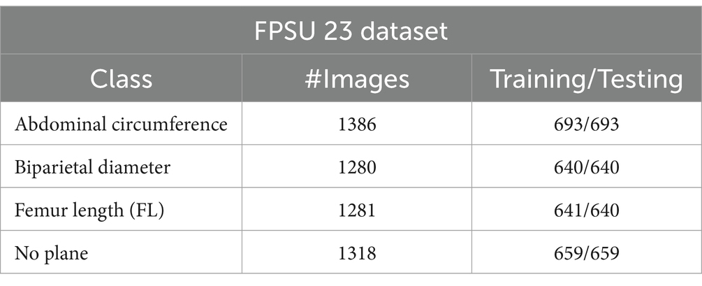
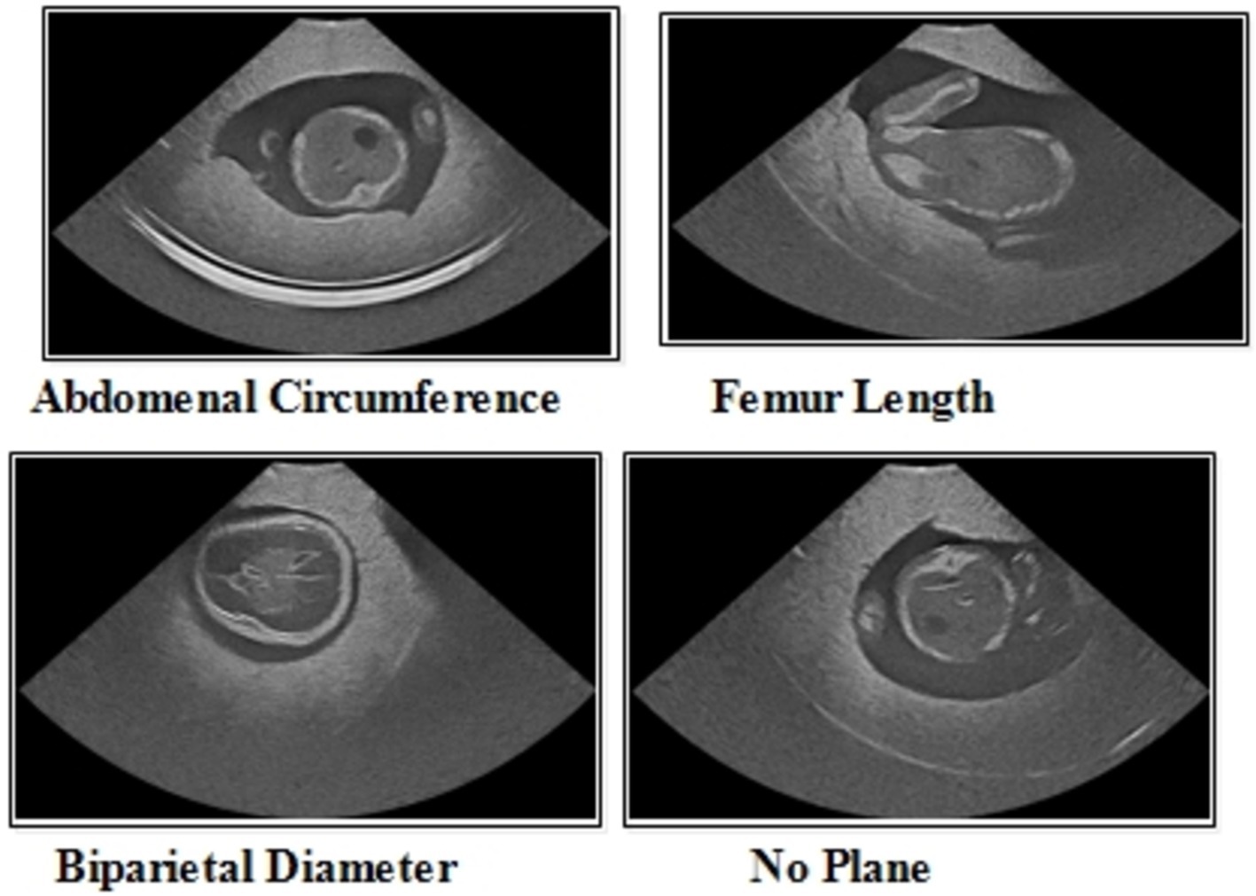
The FPSU23 was developed in 2023 and consists of four classes (18). The four classes are Abdominal Circumference (AC), Biparietal Diameter (BPD), Femur Length (FL), and No Plane. As described in Table 1, the number of images differs throughout classes, as showed in Figure 2.
Abdominal circumference (AC): The abdominal circumference measures the widest part of the abdomen and is used in healthcare for various purposes, including assessing adult abdominal fat and monitoring fetal growth during pregnancy.
Biparietal diameter (BPD): Prenatal ultrasounds utilize the biparietal diameter (BPD) measurement to assess fetal head size and development, involving the distance between major parietal bones on the fetal skull. This measurement aids in gestational age assessment during the early to mid-second trimester.
Femur length (FL): FL measurement in prenatal ultrasounds tracks fetal thigh bone length, assisting in gestational age estimation and growth monitoring, focusing on the second and third trimesters for gestational age determination.
3.1.2 Fetal dataset
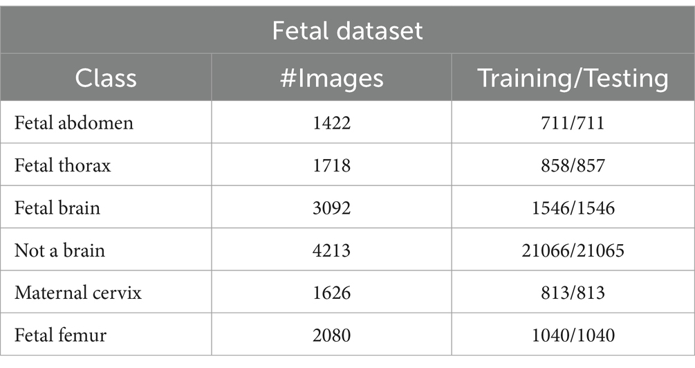
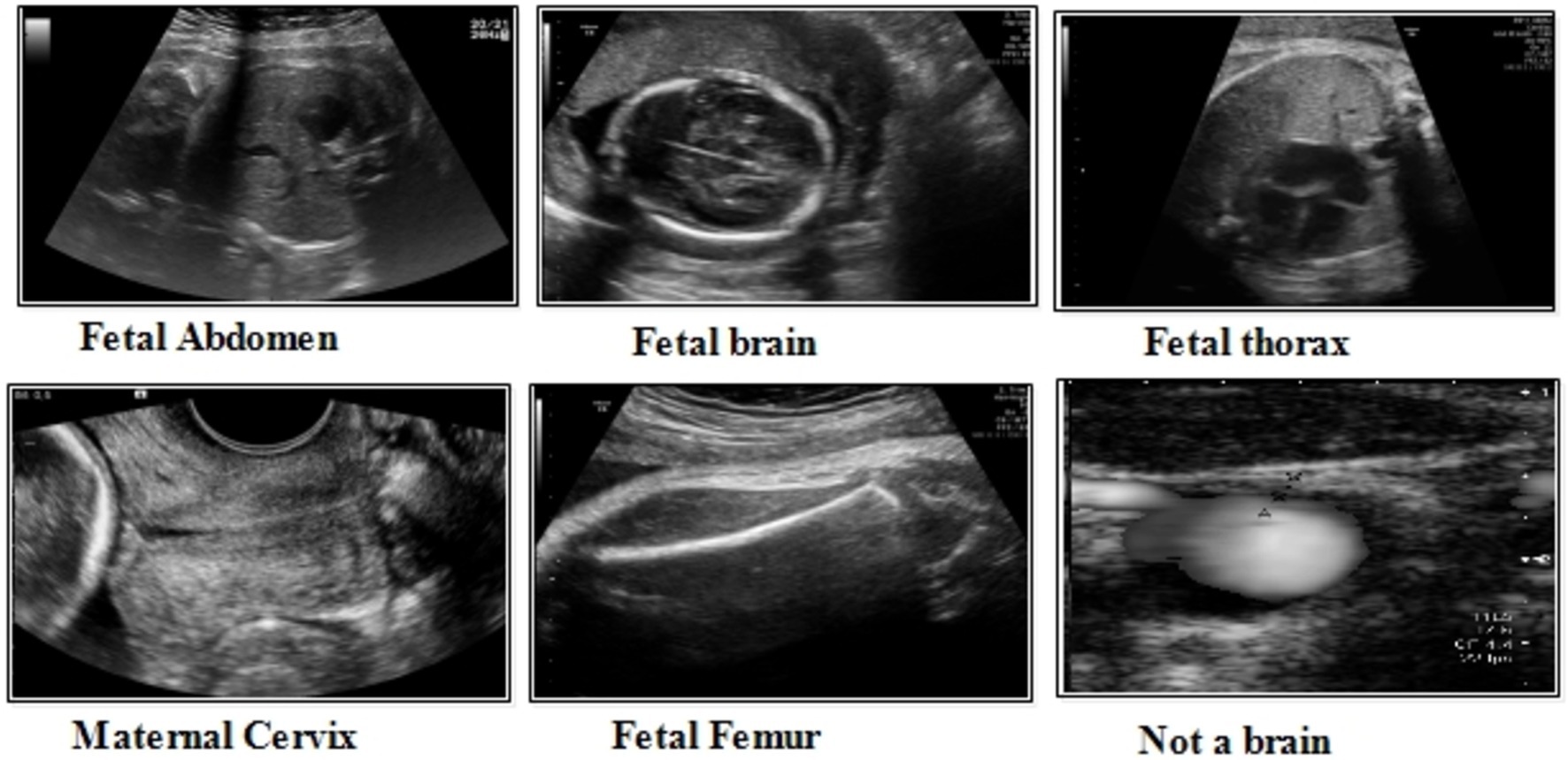
This dataset includes six classes: fetal abdomen (FA), fetal brain (FB), fetal femur (FF), fetal thorax (FT), maternal cervix (MC), and not a brain (NB) (44). The fetal abdomen consists of 1422 images; Fetal Thorax contains 1718 images; fetal class includes 3092 images; maternal cervix consists of 1626 images; and the fetal femur contains 2080. As described in Table 2, the number of images differs throughout classes, as showed in Figure 3.
Fatel brain: As the fetal brain develops from the neural tube during pregnancy, it continues to develop into early childhood, affecting cognitive and motor development. Ultrasound and MRI are crucial tools for detecting fetal abnormalities during pregnancy.
Fatel thorax: An unborn infant’s fetal thorax contains respiratory and circulatory tissues from neck to abdomen. Monitoring this region can identify potential respiratory or circulatory issues and abnormalities.
Maternal cervix: During pregnancy and childbirth, the maternal cervix extends into the vaginal canal and plays a crucial role. For predicting premature labor, monitoring its length and condition is critical to assessing the risk of premature birth and tracking cervical changes.
3.2 Proposed three-residual blocks CNN
Residual blocks are a fundamental architectural component in deep neural networks, particularly in the context of convolutional neural networks (CNNs). They were introduced as part of the “ResNet” (Residual Network) architecture by Jian et al. (45). In deep networks, residual blocks address the problem of vanishing gradients, which can hinder training and limit their ability to learn complex features. In a residual block, the input to a layer is passed through that layer and directly to subsequent layers. This introduces a shortcut connection that bypasses one or more layers, allowing the network to retain and propagate gradient information more effectively during training. The motivation for choosing residual blocks because it facilitate the learning of deeper architectures by enabling the network to preserve important feature information through skip connections, ensuring better gradient flow. In the specific domain of fetal image classification, deeper networks with residual connections allow the model to capture more complex patterns without increasing the computational cost, making them highly relevant for achieving accuracy while maintaining efficiency.
The structure of a residual block typically involves three main components: the input path (the original input to the block), the residual path (which processes the input through a series of layers), and the skip or shortcut connection (which directly adds the input to the output of the residual path). The result is that a residual block aims to learn the residual (the difference between the input and the output), making it easier for the network to fine-tune the learned features. Maintaining a stride of 1 across all layers is vital in residual block to enable parallel fusion. This ensures compatibility between the sequence of various layers before addition and the layers within the block, requiring the size of the last layer in the set and the last block layer to match.
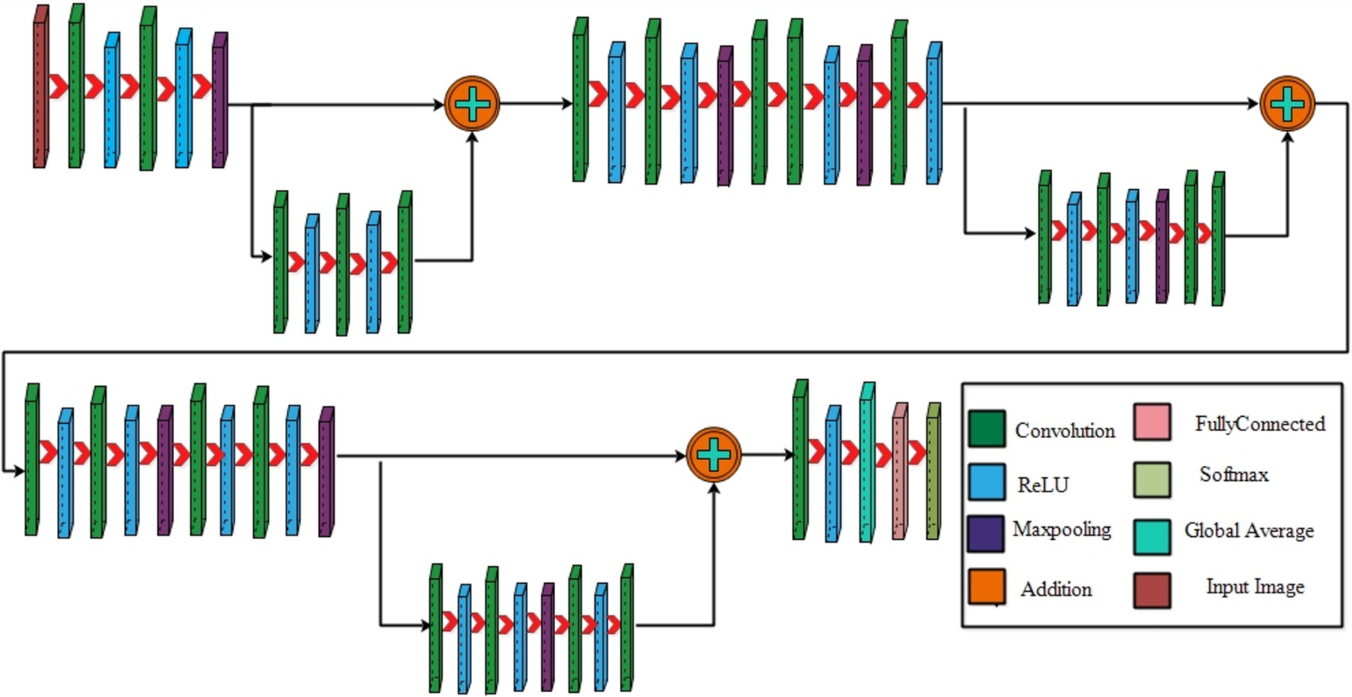
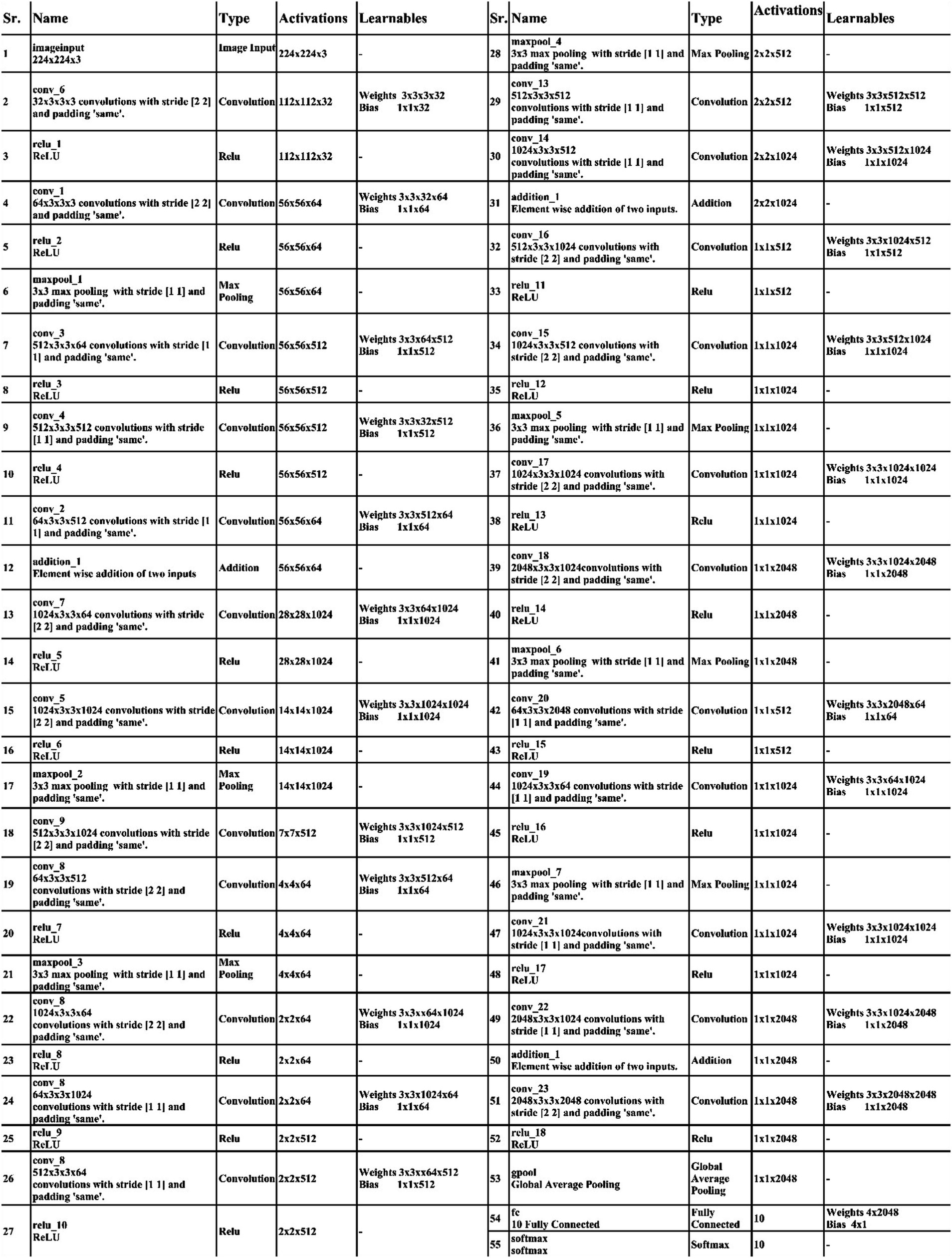
Initiating with an input layer sized at 224 × 224 × 2 and a depth of 3. The network begins with a convolutional layer configured with the following parameters: a depth of 32, a kernel size of 3 × 3, and a stride of 2. These values correspond to the number of filters (depth), the size of the receptive field (kernel), and the step size (stride) used to move the filter across the input. A relu activation layer is applied following each convolutional layer to introduce nonlinearity and boosting the network’s ability to recognize intricate patterns and preventing the loss of learning strength by nullifying negative values. The next step in the process is to add another convolutional layer with a depth of 64, 3 × 3 filter and a stride of 2. To reduce the spatial dimensions while preserving essential features, a Relu activation layer and a max pooling layer having 3 × 3 with stride 1 follow. Then, the first residual block is appended, consisting of five layers. The initial two convolutional layers have 512 depth, 3 × 3 filter and stride 1. A pair of relu activation layers are positioned after each convolutional layer. Concluding this block, an extra convolutional layer with a depth of 64, 3 × 3 filters, and a stride of 1 is integrated. An addition layer is introduced to establish connections, merging data through element-wise addition, thus augmenting the network’s capacity to comprehend relationships and intricacies. After this, two additional convolutions are applied, with each convolution followed by two relu activation layer. Both layers maintain a depth of 1024 and employ a filter size of 3 × 3 with a stride of 2, as shown in Figure 4. A detailed architecture is shown in Figure 5. Both layers keep a depth of 1024 and utilize a filter size of 3 × 3 with a stride of 2. A max pooling layer with a filter size of 3 × 3 and a stride of 1 is added. Subsequently, two convolutional layers are appended, one with a depth of 512 and the other with 64. Both maintain a filter size of 3 × 3 and a stride of 2. Another max pooling layer with a filter size of 3 × 3 and a stride of 1 follows. A convolutional layer and Relu layer pair are included before the subsequent residual block is added. Then a convolutional with 1024 depth, 3 × 3 filter and stride of 2 added. The second residual block is integrated in this step, featuring seven layers. The first convolutional layer, accompanied by a Relu layer, maintains a depth of 64, a filter size of 3 × 3, and a stride of 1. A pair of convolutional and Relu layers follow, both have 512 depth, 3 × 3 filter, and a stride of 1. A max pooling layer with a filter size 3 × 3 and a stride of 1 ensues. Concluding the second residual block are two convolutional layers, one with 512 depth and the other with 1024. Both layers possess 3 × 3 filter and a stride of 1. The second addition layer integrates the residual block and the layers (Figures 6, 7).
Two convolutional layers, each with a subsequent Relu layer, are implemented next. Both layers maintain a 512 depth, stride 2 and 3×3 kernel size. Following these, two convolutional with accompanying relu layers are inserted. Both layers have a depth of 1024, 3×3 filter, and a stride of 2. A max pooling layer with 3×3 filter and a stride of 1 follows. A convolutional layer, followed by a Relu layer, is then appended with a depth of 2048 and a stride of 2. Subsequently, a max pooling layer with 3×3 filter and a stride of 1 is added. The third addition layer concludes this set. The third residual block, consisting of eight layers, is introduced. The initial convolutional layer, accompanied by a relu layer, maintains a depth of 64, 3×3 filter, and a stride of 1. Following this, convolutional and Relu layers are incorporated, each holding 1024 depth, 3×3 kernel with stride 1. A max pooling layer with a filter size of 3×3 and a stride of 1 ensues. Subsequently, another pair of convolutional and Relu layers are included. The convolutional layer holds 1024 depth, 3×3 kernel size with stride 1. Concluding the third residual block is a convolutional layer with a depth of 2048, 3 × 3 kernel, with stride 1. The final step involves the addition of a pair of convolutions, each accompanied by a following relu layer, with a depth of 2048, 3 × 3 kernel, with stride 2. Lastly, the deep neural network concludes with a global average pooling layer, a fully connected layer, and a Softmax layer. In the proposed architecture, the loss was calculated using the cross-entropy loss function. This function is extensively used in classification problems since it calculates the difference between the projected probability distribution and the true labels, effectively assessing the model’s performance. The training loss for the 3-residual block model on the FPUS23 dataset was 5.7, whereas it measured 24.8 for the fetal dataset.
3.2.1 Four-residual block CNN
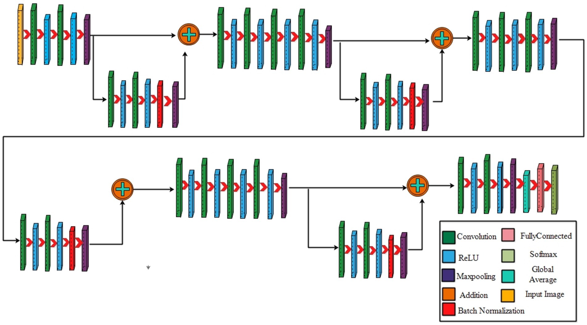
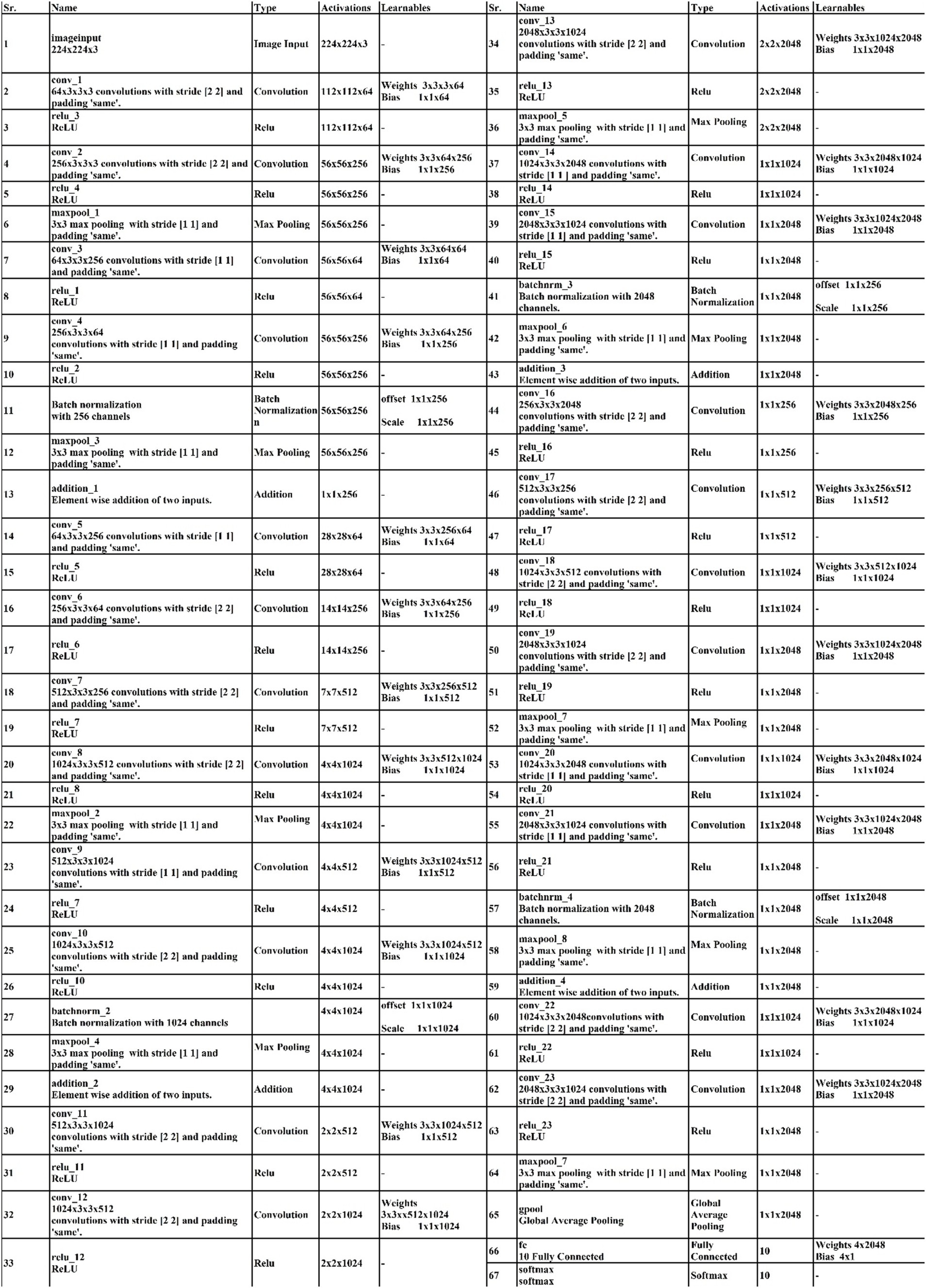
The proposed 4-residual blocks CNN architecture consists of 4-residual blocks, with each block comprising multiple layers, and few of them are different from 3-residual blocks CNN. The first input layer of this architecture has a size of 224 × 224 and a depth of 3. A convolution layer included has 64 depth, 3 × 3 kernel size with stride 2. After convolution layers, a relu layer is incorporated; then second convolution added with 256 depth, 3×3 filter, and a stride of 2. This is succeeded by a relu layer with max pool, utilizing 3 × 3 kernel and a stride 1.
The first residual block, which has a total of six layers, is then added after that. The initial two convolutional exhibit 64 and 256 depth, both utilizing the 3×3 filter and stride value 1. Each convolutions is followed by a strategically placed set of relu layers, which introduce non-linearity into the network. A subsequent addition is a batch normalization layer boasting 256 channels. At the end of the first residual block, the addition of a max pooling layer comes into play, featuring 3 × 3 kernel with stride 1. The first addition layer combines the residual block and set of layers.
Following the initial convolution, a relu layer was added with a 64 depth size, 3 × 3 filter, with stride 2. Next, two convolutional layers were introduced, with depths of 256 and 512, using a 3×3 filter size and maintaining a stride of 2. After each convolutions, a set of relu layers was strategically placed. Another convolutional layer, followed by a relu layer, was added with a 1024 depth, 3 × 3 filter with stride 2. Lastly, a max pool added with 3 × 3 kernel.
The second residual block, which has six layers, is added at this step. The initial two convolutional layers exhibit depths of 512 and 1024, both utilizing 3 × 3 kernel with 1. Following each convolutional layer, a set of Relu layers is thoughtfully positioned to infuse non-linearity. A subsequent addition is a batch normalization layer boasting 1024 channels. At the end of the first residual block, the addition of a max pooling layer comes into play, featuring 3 × 3 kernel and stride 1. The second addition layer combines the residual block and set of layers.
After this, the first convolutional layer with the following Relu was added with 512 depth, 3 × 3 filter, and stride size 2. After this, two convolutions exhibit depths of 1024 and 2048, utilizing the same 3 × 3 filter and maintaining a stride of 2. At the end of this set, a max pooling layer has been added.
The third residual block, which has six layers, is then added. The initial two convolutional layers exhibit depths of 1024 and 2048, utilizing the 3 × 3 kernel. Following each convolutional layer, a set of Relu layers is thoughtfully positioned to infuse non-linearity. A subsequent addition is a batch normalization layer boasting 2048 channels. At the end of the first residual block, the addition of a max pooling layer comes into play, featuring 3 × 3 kernel and a stride of 1. Now, the third addition layer combines the residual block and set of layers. The 4th residual block, which has six layers, is added at this step. The initial two convolutional layers exhibit depths of 1024 and 2048, utilizing the same 3 × 3 kernel. After convolution layers, a set of relu activation is thoughtfully positioned to infuse non-linearity. A subsequent addition is a batch normalization layer boasting 2048 channels. At the end of the first residual block, the addition of a max pooling layer comes into play, featuring 3 × 3 kernel size with 4th addition layer combines the residual block and set of layers.
At the end of this model, a convolution with the following relu layer added has 1024 depth, 3×3 kernel size, and stride 2. Next again, a convolution with the following rule’s has been added with 2048 depth and has same kernel. Then a max pool layer having 3 × 3 kernel added. Then, the global average pooling layer is fully connected, and the Softmax layer has been added. The training loss for the 4-residual block model on the FPUS23 dataset was 4.9, with a corresponding value of 18.8 for the fetal dataset. The proposed 3-Residual and 4-Residual-block models differ from pre-trained architectures such as ResNet18 and ResNet50 in terms of both design and parameter efficiency. 3-Residual block model has 3.77 million parameters, significantly fewer than ResNet 18’s 11.7 million parameters. It incorporates only three residual blocks, prioritizing computational efficiency without sacrificing accuracy and 4-Residual-block model has 18.87 million parameters which is fewer than ResNet50 model 23.5 million parameters. The reduced number of parameters leads to faster training and inference times, making it a lightweight alternative to deeper models.
3.3 Selecting hyperparameters
In this work, we use Bayesian Optimization (BO) to select hyperparameters values employed in the proposed architecture for the training process. Bayesian optimization was selected due to its efficiency in identifying optimal parameters with fewer evaluations, compared to methods such as the grid search algorithm. BO builds a probabilistic model to explore the hyperparameters space intelligently, concentrating on promising regions and avoiding exhaustive searches. BO offers a more effective solution for deep networks, where each evaluation can be computationally intensive. By contrast, grid search and other algorithms. The 3-residual-block model has been trained with 3.77 million hyper parameters, while the 4-residual-block model has been trained with 18.87 million hyper parameters. The optimization of DL architectures comprises a black box optimization process, where the objective function is a black box function. The main aim of BO is to obtain the values of hyperparameters that help improve the accuracy of training models than inexpert researchers. The process of BO is defined under the following six steps.
• By employing the Gaussian Process, the posterior distribution is adopted to update the previous results of a black box function . Mathematically, the Gaussian Process function is defined by Equation 1.
Where denotes the mean function and covariance function .
Using an acquisition function, the optimal point for the function is selected using the expected improvement as the acquisition function, which is defined by Equation 2.
• Using , we trained to maximize the w.r.t. current optimal value . Mathematically, it is defined by Equation 3.
• The objective function is utilized to find the validation set results.
• Augmenting the best-optimized sample points to the data already selected.
• The statistical Gaussian Process model is finally updated.
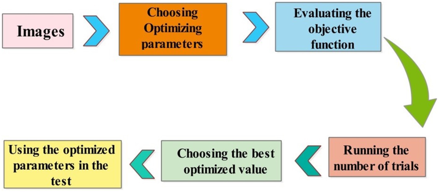
Iterations are repeated until a maximum number is reached. In this paper, we selected several hyperparameters after employing BO (see Table 3). In addition, the visual process of BO is shown in Figure 8.
3.4 Training the proposed model and extracting features
On the chosen datasets, both proposed architectures have been trained using a ratio of 50 and 50 in the training process. Several hyperparameters (HPS) have been used in the training process, as mentioned in Table 3. The hyperparameters settings determine the training of the models, which is followed by the extraction of features based on the learned features. Throughout the training process, features are extracted from the global average pooling layer of the trained models. The extracted features are analyzed at this stage, and it was observed that some irrelevant information is included that should be removed for the final classification. Global average pooling layer is used for feature extraction and we obtain two feature vectors from 3 residual block model and from 4 residual block model of dimensions . We proposed an improved feature selection method named the Improved Generalized Normal Distribution Optimization (IGNDO) algorithm to resolve this issue.
3.5 Improved feature selection algorithm and fusion
In real-world problems, population-based methods provide efficient solutions using artificial intelligence (AI) (46). Optimization techniques encompass both gradient and non-gradient approaches. In this work, we implemented an improved version of the Generalized Normal Distribution optimization called IGNDO. The improved GNDO algorithm is applied on these feature vectors separately and then obtained two best feature vectors that contain only important information (best features).
Generalized normal distribution optimization (GNDO): The GNDO emerges as an efficient technique without requiring fine-tuning of initial parameters. In 2020 (47), a noteworthy addition to the realm of optimization algorithms emerged as the GNDO algorithm. Various sophisticated mathematical models were used to develop this innovative algorithm, all based on the elegant concept of normal distributions. The algorithm is an example of metaheuristics, which takes inspiration from classical normal distributions. A diverse array of mechanisms is employed by the GNDO algorithm to perfectly balance the key dynamics of exploration and exploitation within its framework. This fusion of mathematical precision and creative imagination represents a significant advancement in optimization techniques. The Gaussian distribution, commonly called the normal distribution, is a fundamental tool for characterizing natural phenomena. An outstanding feature of the GNDO algorithm is its avoidance of specific controlling parameters, instead relying solely on determining essential population size and terminal condition before its execution. Furthermore, the algorithm’s simplicity shines through its uncomplicated structure, where individual positions are updated using a formulated generalized normal distribution (48).
We can define a normal distribution like this: Suppose there is a random variable , which adheres to a probability distribution defined by the location parameter (μ) and the scale parameter (δ). The expression of its density function for probability takes the form:
Here’s how we can describe a normal distribution: Imagine there is a random variable , which can be denoted as a normal distribution, specifically . As Equation 4 indicates, a normal distribution involves two key variables: the location parameter μ and the scale parameter δ. These parameters, μ and δ, represent the average value and the standard deviation of random variables, respectively.
Searching through a population-based optimization method is divided into three major stages. Initially, individuals are scattered widely. Later, they begin employing strategies that balance global and local solutions, moving toward the ideal global solution. As a result, the individuals come together to identify the best solution. This search process can be likened to the behavior of multiple normal distributions. All individuals’ positions are determined by random variables with a normal distribution. During the initial phase, there is a significant difference between the average position of individuals and the optimal solution’s location. Simultaneously, a variation in the positions of all individuals is also relatively high at this point. As the process advances into the second phase, the difference between the average and optimal solution positions systematically lessens.
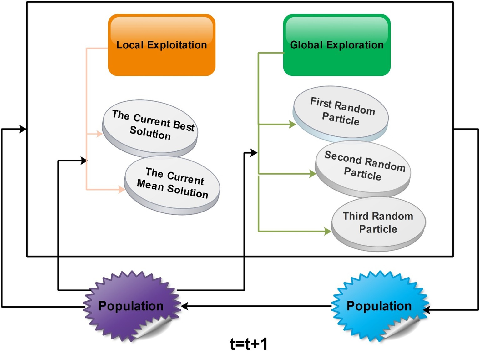
Similarly, the variability in individuals’ positions starts decreasing. In the final phase, the distance between the average position and the optimal solution’s location and the variability in individuals’ positions reach their lowest points. This signifies the population’s convergence around the most optimal solution. A visual framework of GNDO is shown in Figure 9.
GNDO features a straightforward framework in which local exploitation and global exploration represent the core information-sharing mechanisms. The execution of GNDO relies on developing local exploitation and global exploration strategies. Local exploitation revolves around a generalized normal distribution model that has been established and is directed by the current mean and optimal positions. On the other hand, global exploration involves three individuals chosen randomly. These two strategies carry equal significance in GNDO and have equal selection probabilities. GNDO stands out for its minimal requirements: specifying population size and termination conditions before starting. After evaluating individual performance using an objective function, the algorithm iterates, using random numbers to transition between exploration and exploitation until the end criterion is met. Moreover, similar to other optimization algorithms based on populations, the GNDO population is initialized using the Equation denoted as Equation 5:
Here, represents the count of design variables, signifies the position of the ith individual at time , the symbol denotes the lower limit of the design variable, signifies the upper limit of the design variable, and λ5 is a randomly generated number ranging between 0 and 1. The obtained outcomes are subject to analysis using a Wilcoxon signed-rank test, considering a significance level of α = 0.05.
3.5.1 Local exploitation
Local exploitation pertains to the quest for better solutions within the immediate positions of all individuals scattered throughout the search space. To commence, the algorithm initiates by generating a random population; this is achieved by applying the subsequent Equation 6:
The population size, denoted as , is coupled with the trial vector for the ith individual at time . The generalized mean position of the individual is represented by , while δi stands for the generalized standard variance. Additionally, the role of η comes into play as the penalty factor.
Here, represent random values falling within the range of 0–1 and refers to the current best position. The symbol refers to the mean of the average position in the existing population, which can be determined by applying the following Equation 10:
It is important to acknowledge that the individual represented by might not always discover an improved solution through local exploitation or global exploration strategies. A screening procedure was introduced to ensure the integration of better solutions into the next generation’s population. This procedure can be formulated as follows:
3.5.2 Mean position
The Generalized Mean Position (GMP) concept involves adjusting individuals’ positions within a population during optimization. The best individual contains valuable global solution information, and others are guided toward its direction. This can lead to premature convergence if gets trapped locally. Mean position is introduced to mitigate this, allowing individuals to move between and , improving solution discovery. The changing enhances adaptability, which reduces the risk of local maxima, making it a valuable addition to local exploitation strategies.
3.5.3 Standard variance
In the realm of GNDO, the infusion of the Generalized Standard Variance δi concept significantly amplifies its local search proficiency. It functions as a fluctuating sequence of randomness, directing exploration toward the Generalized Mean Position . The distance that exists among an individual’s location (like yt [i]) and key points like the Mean Position (M) and top performer ( ) impacts the fluctuations of this sequence. A more considerable distance leads to more substantial changes, helping struggling individuals discover better solutions. Conversely, for individuals already performing well, a gentler fluctuating sequence aids in finding even more optimal solutions nearby.
3.5.4 Penalty factor
The penalty factor contributes to the generalized standard variance’s generated randomness in the GNDO algorithm. This factor influences the resultant random sequence. Most penalty factors tend to fall between −1 and 1. It is important to emphasize that the generated generalized standard variances are consistently positive. This penalty factor’s impact expands the search directions within GNDO, thus strengthening the algorithm’s overall search capabilities.
3.5.5 Global exploration
Global exploration involves searching the solution space on a broad scale to identify promising areas. In GNDO, this exploration is carried out by selecting three individuals at random, as illustrated in the following Equation:
Here, and represent two random numbers following a standard normal distribution. The parameter ß denotes the adjustment parameter and takes on a random value between 0 and 1. Additionally, v1 and v2 stand for two trail vectors. Furthermore, the computation of v1 and v2 can be accomplished using the following equations:
Here, , , and represent three distinct random integers chosen from 1 to , satisfying the condition . By employing Equations Equation 13 and 14, the second term on the right side of Equation 12 can be termed as the “local learning term,” indicating the exchange of information between solution and solution . The third term on the right side of Equation 12 can be called “global information sharing,” signifying that individual receives information from individuals and . The adjusted parameter ß is utilized to balance these two information-sharing strategies. Furthermore, and denote random numbers following a standard normal distribution, broadening GNDO’s search scope during global search operations. The absolute symbol in Equation 12 maintains consistency with the screening mechanism defined in Equations 13 and 14.
3.5.6 Global search with binary cross entropy
The global search matrix is computed and later utilized to handle the uncertainty using the binary cross-entropy function. The binary cross-entropy function is defined as follows:
Where denotes the global search matrix obtained using Equations 12–14, the global search matrix is employed for the entropy value calculation using Equation 15. The entropy value is computed in 1, 0 form that shows the either global feature is selected (1) or not (0). The threshold function is defined as follows to get the final feature vector.
Where is a selected feature vector and is a feature vector containing features that do not meet the selection criteria. A pseudo-code for the IGNDO algorithm is given in Algorithm 1. As an input, population size is defined as , variable upper limit and lower limit of variables l; the starting iteration count T = 0, and the maximum iteration limit all be considered. The stopping criteria of this algorithm are defined based on the number of iterations. In our case, we performed 200 iterations.
ALGORITHM 1 Best features selection using IGNDO algorithm
1. Using Equation 5, initialize an individual from the population.
2. Calculate the fitness value of every individual and achieve the best solution .
3. The number of iterations t is updated to t + 1
\*Main Loop*\
4. While T < Tmax do
5.for i = 1 to N
6.Generate a random value, denoted as α, within the range of 0 to 1.
7.if >0.5
\*Local exploitation strategy*\
8.Equation 10 calculates the mean position M by choosing the optimal solution ybest.
9.Equations 7–9, respectively, were used to calculate the generalized mean position, generalized standard deviation, and penalty factor.
10.Computer the local exploitation strategy.
11.else
\*Global exploration strategy*\
12.Execute a global exploration strategy by using Equation 11–14
13. Find the entropy of the global search matrix using Equation 15.
14. Entropy features are passed in a final threshold function Equation 16.
15.end if
16.end for
17. Increment the current iteration number by: t = t + 1.
18. end while
Output: The optimal solution y best.
The above algorithm is applied separately to both proposed models’ extracted deep features. The learning rate for Stochastic Gradient Descent with Momentum (SGDM) in this work is set to 0.000274, which is a crucial parameter controlling the step size during weight updates and influencing the convergence of the model. In the end, we obtained two feature vectors of dimension and respectively. The selected features are finally fused using a simple serial-based approach and get the accuracy. The resultant serially fused vector has a dimension of . In the final step, the fused vector is passed to the neural network classifiers to compute the final accuracy. Five neural network classifiers have been selected for the classification results as narrow-neural network (N3) (49), medium-neural network (MN2) (50), wide-neural Network (WN2) (51), bilayered-neural network (BN2) (52), and trilayered -neural network (TN2) (53).
4 Results and discussion
The results of the proposed method are discussed here with a detailed numerical analysis and confusion matrix. The results are computed on selected datasets using 10-fold cross-validation. There were two equal parts of the dataset, with 50% allocated for training and rest 50% allocated for testing. The proposed fusion architecture is trained on the fetal dataset and FPSU23 dataset; however, some hyperparameters are needed to train deep architecture and optimization algorithms. All training hyperparameters have been discussed in Table 3. The optimization algorithm selects 20 populations and 200 iterations for the best feature selection. The validation determines the best model based on performance metrics, including precision, accuracy, time, recall, FNR, MCC, F1-sc and kappa. Multiple classifiers are employed for validation, focusing on achieving the highest accuracy and minimum processing time. An MATLAB 2023b workstation equipped with 128GB RAM, a 512GB SSD, and a 12GB NVIDIA RTX 3060 graphics card was used to simulate the proposed architecture.
4.1 Experiments of the proposed architecture
To validate the proposed structure, a number of experiments were conducted:
Deep features extraction (54) from GAP (global average) layer of proposed 3-Residual block CNN.
• Deep features extraction from GAP (global average) layer of proposed 4-residual block CNN.
• Feature Selection (55) by employing improved GNDO for 3-Residual block deep features.
• Feature Selection by employing improved GNDO for 4-residual block deep features.
• Fusion of best-selected features using serial approach.
• Classification (56) by applying neural network classifiers.
4.2 FPSU23 dataset
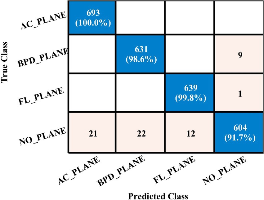
Table 4 demonstrates the classification results achieved using the 3-Residual block model on the FPSU23 dataset. The trained model’s features are extracted, and classification is performed. The MN2 classifier obtained the best accuracy of 97.5%. Additional performance metrics for this classifier include 97.52 percent recall, 97.55 percent precision, 0.99% AUC and 97.53% F1-sc. The confusion matrix for MN2 is shown in Figure 10 that can be utilized to verify the correct prediction rate of each class. Furthermore, the confusion matrix can be used to check the computed performance metrics. During testing, 44.98 s was the lowest measured time for the MN2 classifier, while the TN2 highest recorded time is 134.97 (sec). The rest of the classifiers also obtained the accuracy values of 97.3, 97.5, 97.1, and 96.9, respectively.
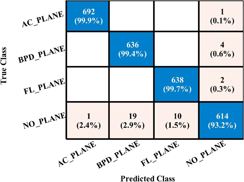
Table 5 presents the results of the proposed 4-residual block deep features for the FPSU23 dataset. The best-obtained accuracy for this model is 98.0% for the WN2 classifier. Also the recall is 98.05%, precision 98.05%, F1-sc 98.05%, and AUC 0.99%. Figure 11 shows the confusion matrix of this classifier that can be utilized to verify the correct prediction rate of each class. Every classifier’s computation time has also been recorded, and it is observed that the WN2 classifier’s least recorded time is 982.34 s, while the TN2 highest recorded time is 499.41 (sec). Compared to the performance of this model with 3-Residual, it is noted that the accuracy is improved, but computationally, the 3-Residual model is better. A feature selection method is implemented on both proposed models to minimize the computational time further.
The classification results following the implementation of an improved GNDO algorithm on 3-Residual Block CNN deep features are presented in Table 6. In this table, the best-obtained accuracy is 97.6% for MN2. The values of other calculated measures include a recall rate of 97.62%, precision rate of 97.62%, F1 Score of 97.62%, and AUC value of 0.99%, respectively. Comparing the results of this experiment with Table 4, it is observed that the accuracy is improved, and time is significantly reduced. The MN2 classifier’s least recorded time was 20.57 s after selecting the best features and 44.98 s before the selection process. A proposed classification method result is presented in Table 7 after using the improved GNDO algorithm on 4-residual blocks CNN deep features. After employing this experiment, the best-obtained accuracy of 98.0% has been achieved for N3. The recall is 97.75%, precision 98.05%, F1-sc of 97.89%, and AUC value of 0.99% obtained for this classifier are better than the performance noted in Table 5. The computational time is also reduced for this experiment, and it is observed that the overall accuracy is also improved, which shows the strength of this method. The N3 classifier’s least recorded time is 49.08 s after selecting the best features.

Table 6. Feature selection by improved GNDO algorithm of 3-residual blocks model using FPSU23 dataset.

Table 7. Feature selection by improved GNDO algorithm of 4-residual blocks model using FPSU23 dataset.
Ultimately, the optimal characteristics from both models were combined, and Table 8 displays the outcomes. With respect to recall, precision, and F1 score, MN2 yielded the best accuracy of 98.5, 98.52, 98.55, and 98.53%, respectively. Improved accuracies of 98.1, 98.3, 98.1, and 98.4% were attained by the remaining classifiers. The confusion matrix of MN2 following the fusion procedure is displayed in Figure 12, which can be used to confirm the overall performance metrics. While the first experiment’s maximum accuracy was 97.5%, the second experiment’s maximum accuracy was 98.0%, the third experiment’s maximum accuracy was 97.6%, the fourth experiment’s maximum accuracy was 98%, and the fifth experiment’s maximum accuracy was 98.5%. Hence, overall, the proposed framework and the optimization process show improvement after the fusion process.
4.3 Fetal dataset results
The classification results of the fetal dataset using the proposed architecture have been presented in this subsection. The proposed results are computed in several experiments, as discussed in the above section. The results of the first experiment are presented in Table 9, showing the maximum accuracy of 78.3% for the WN2 classifier. Other measures are recall 77.75%, precision 77.28%, the F1-sc 77.51%, kappa 0.1922, and MCC 0.7194, respectively. The rest of the classifier obtained an accuracy of 76.0, 77.1, 75.9, and 75.2%, respectively. Computationally, this architecture is a little expensive, as the minimum noted time is 268.29 (sec). Table 9 (2nd quarter) illustrates the classification results for the proposed 4-residual blocks CNN with deep features. The best-obtained accuracy of this experiment is 84.1% for the MN2 classifier. The kappa and MCC measures are also computed, and the obtained values are 0.4255 and 0.7891. The rest of the classifiers obtained accuracy values of 83.3, 83.9, 83.5, and 83.6%, respectively. The MN2 achieved a high accuracy but consumed 1230.8 (sec) for the execution.
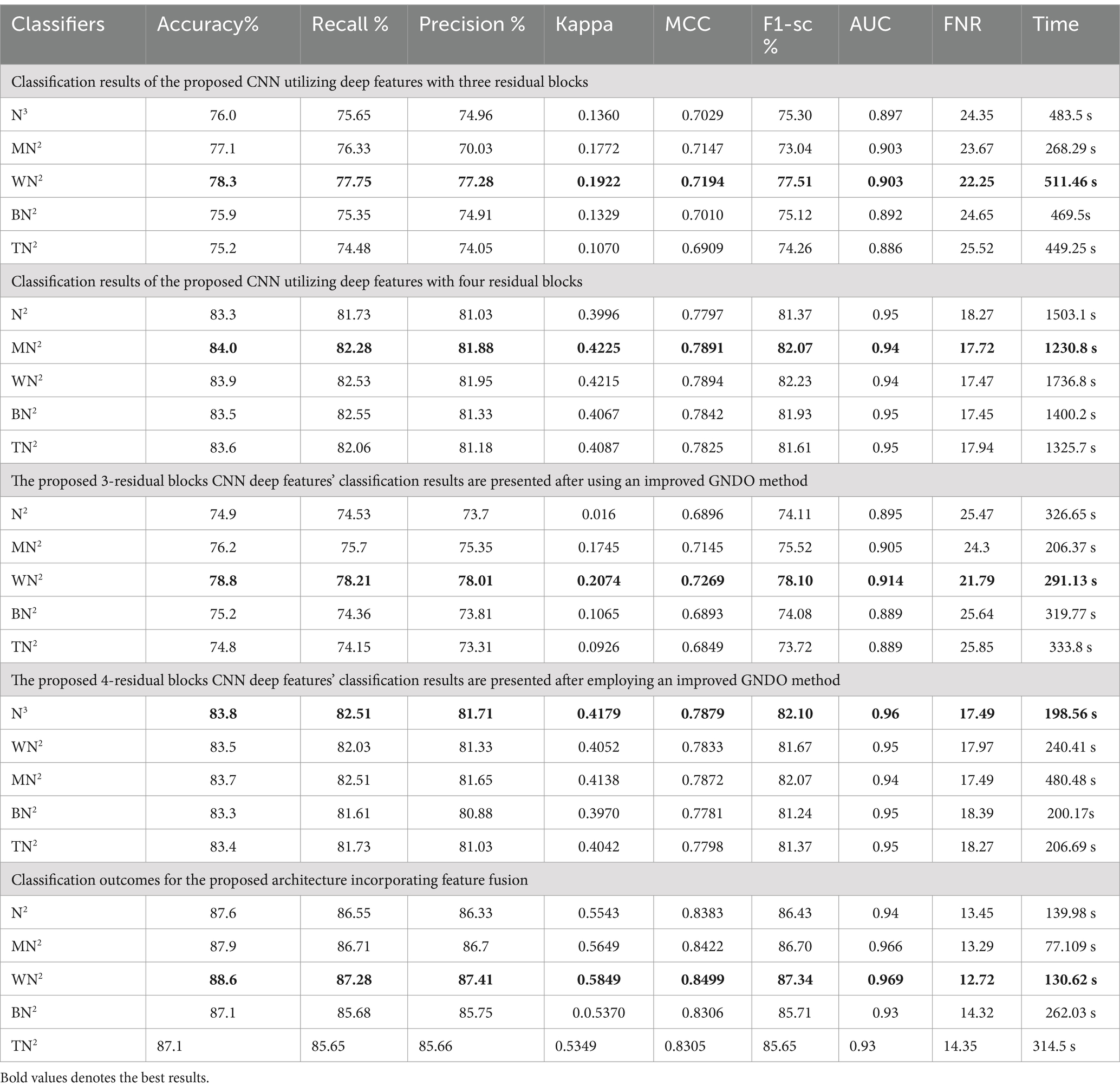
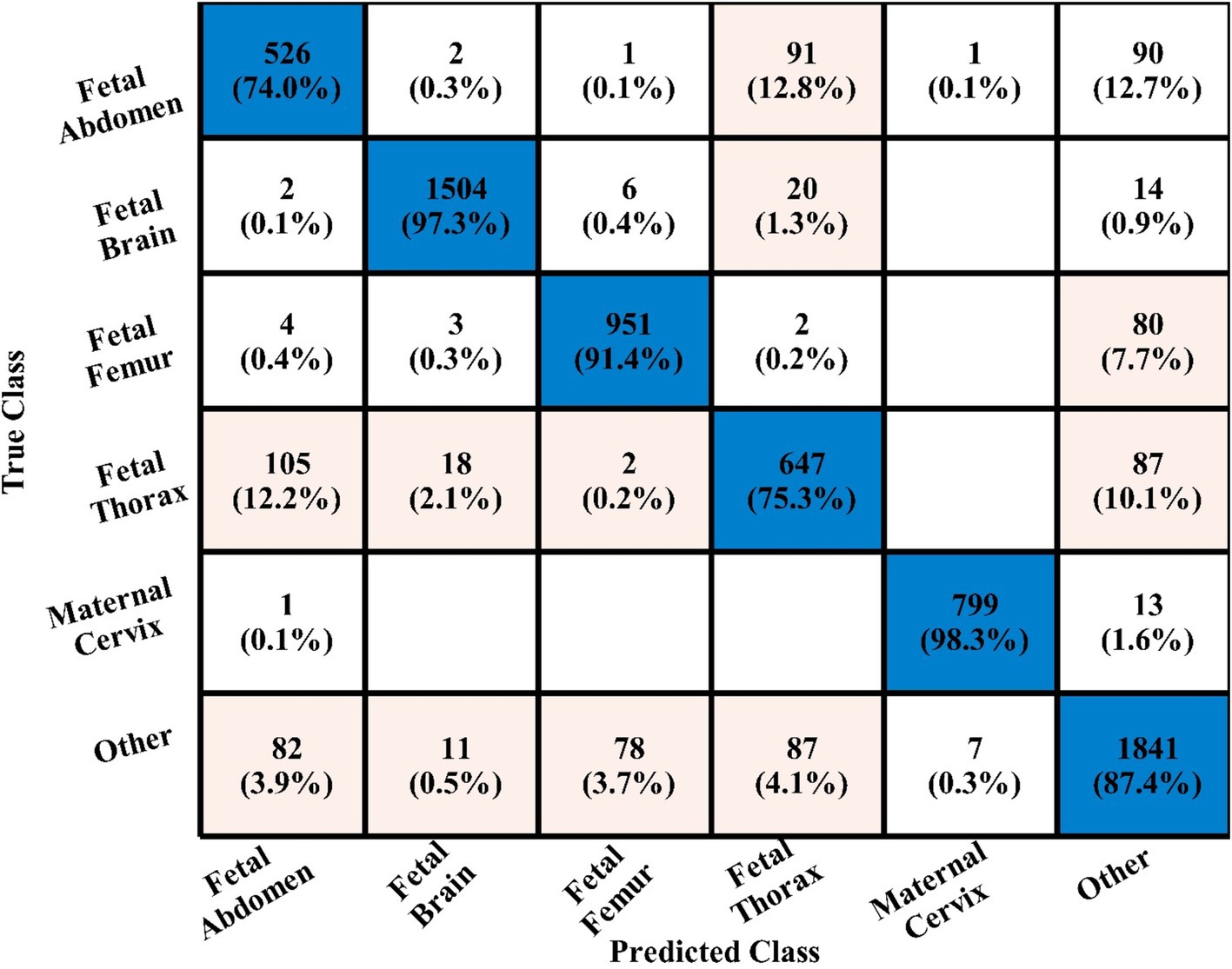
In the third experiment, the feature selection algorithm is applied using three residual blocks CNN deep features, the maximum accuracy was obtained of 78.8% for WN2 classifier. The other computed measures of WN2 classifier, such as recall 78.21%, precision 78.01%, kappa value of 0.2074, MCC value of 0.7269, F1-sc of 78.10%, and AUC value of 0.914%, respectively. The computation time for each classifier is also determined, and MN2 is executed in the maximum processing time of 291.13 s, whereas the minimum noted time is 206.37 s for WN2. Similarly, the feature selection algorithm is applied on 4-residual blocks deep features and obtained an accuracy of 83.8% for N3. This classifier also has other parameters that have been computed, such as a recall rate of 82.51%, precision rate of 81.71%, kappa measure of 0.4179, MCC measure of 0.7879, F1 Score of 82.10%, and AUC 0.96%, respectively. The Narrow Neural Network classifier’s least recorded time is 198.56 s, while the TN2 greatest recorded time is 480.48 (sec). The classification results of the proposed 3- and 4-residual block CNN deep features are shown at the end of Table 9. This table presented the best-obtained accuracy of 88.6% for WN2 classifier. The other calculated measures were recall rate of 87.28%, precision rate of 87.41%, kappa value of 0.5849, MCC value of 0.8499, F1-sc 87.34%, and AUC values of 0.96, respectively. Furthermore, the WN2 confusion matrix is shown in Figure 13 that shows the correct prediction rate of each class (Tables 10–13).
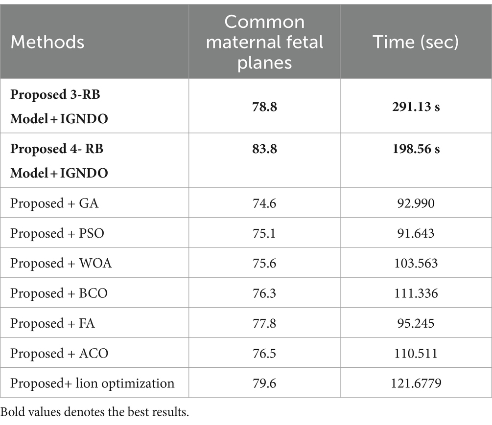
Table 13. Comparison of the two proposed architectures utilizing the fetal plans dataset with a number of other cutting-edge optimization algorithms.
4.4 Discussion
A detail discussion of the proposed method results have been presented in this section. Initially, the t-test has been performed to validate the performance of the selected classifiers. The t-test, a statistical analysis method, is utilized to assess whether there is a significant difference between the means of two groups. When the experiments were finished, the Student’s t-test was used to examine the findings. Two classifiers were first chosen as they both showed constant accuracies during every experiment. This selection made it possible for us to do the experiment using both a low- and high-accuracy classifier, allowing for a comparative comparison. Our initial hypothesis = the accuracy of the chosen classifiers does not vary significantly in a meaningful way. A t-test for the FPSU23 Dataset compared two classifiers: Medium NN and tri-layered NN. The corresponding accuracy of these classifiers is presented in Table 14. For fetal dataset these two classifiers compared: wide NN and tri-layered N2. The corresponding accuracy of these classifiers is presented in Table 14.
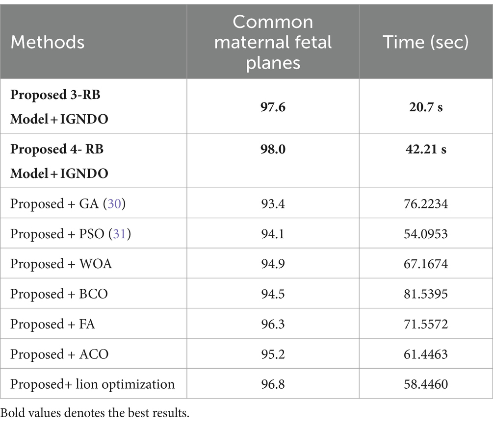
Table 14. Comparison of both proposed architectures with several other state-of-the-art optimization algorithms using FPSU23 dataset.
The difference in their accuracies is calculated using the following formula, where in Equation 17, the term stands for the uppermost accuracy, and stands for the lowermost accuracy. The Mean is evaluated using Equation 18, which is 0.5 for the FPSU23 Dataset and 1.8 for the Fetal Dataset. In this Equation, the denotes a total number of methods.
After that, the standard deviation is computed using the formula shown in Equation 19, and the obtained value is 0.4183 for the FPSU23 Dataset and 1.865 for the Fetal Dataset. After calculating the t-selection value using Equation 20, we found it to be 2.6728 for FPSU23 and 2.15806 for Fetal dataset. These values are used as reference points for conducting the Student’s t-test.
The degrees of freedom are computed as . Assuming the null hypothesis is true at a significance level of 0.05, there is a 5% probability of achieving the observed results, corresponding to a p-value of 0.05. We calculated the confidence interval using the t-test table, considering the p-value and degrees of freedom, resulting in the interval (−2.776, +2.776). The computation of this confidence interval follows the Equation (21).
There is no discernible difference between the two chosen classifiers’ accuracies, as the t-selection value falls within the range based on this confidence interval. Therefore, our hypothesis is accepted.
4.4.1 Comparison with neural nets and SOTA
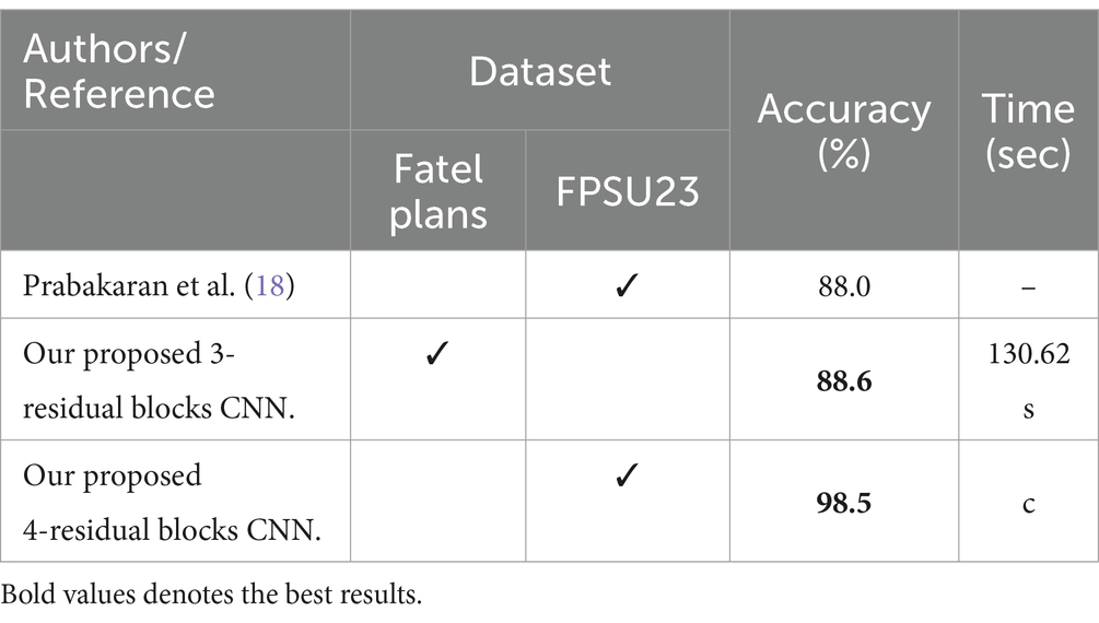
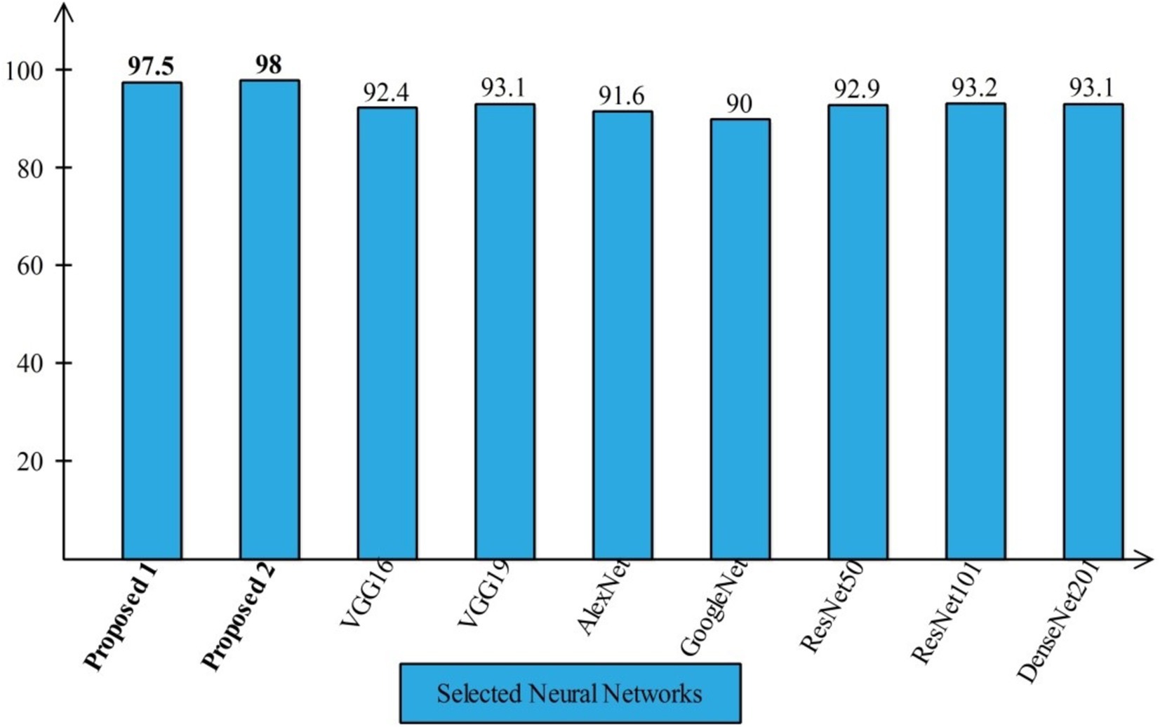
Several state-of-the-art (SOTA) recent deep learning architectures are compared for the two chosen datasets. The methods selected for the comparison is VGG16, VGG19, AlexNet, GoogleNet, ResNet50, ResNet101, DenseNet201, and MobileNet-V2. A comparison is plotted in Figures 14, 15. In Figure 14, the comparison is performed for the FPSU23 dataset that shows the maximum accuracy is obtained by proposed 2 (4-Residual). The maximum accuracy obtained by other pre-trained models is 93.2% of Resnet101. Figure 15 compares the maternal fetal dataset, showing that the proposed 2 (4-Residual) obtained the highest accuracy of 84%. In addition, the authors of the work (18) used the FPSU23 dataset and obtained a maximum accuracy of 88%. However, the proposed method improved overall accuracy of 88.6 and 98.5%, respectively.
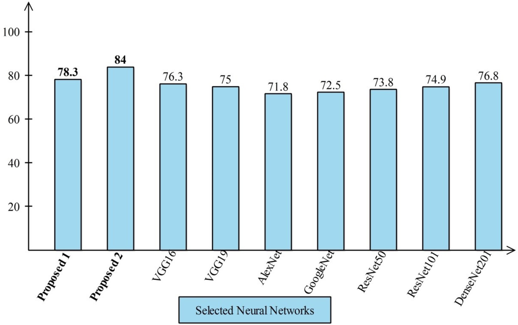
Figure 15. Comparison in term of accuracy for maternal fetal dataset by using several neural networks.
4.4.2 Comparison with other optimization algorithms
An analysis of the improved GNDO in contrast to a few other optimization algorithms inspired by nature. The proposed architecture 3 residual block model obtained the highest accuracy of 78.8% and 4 residual block model 83.8% using the IGNDO algorithm for common maternal fetal planes, as shown Table 13 respectively. The accuracy of the proposed architecture’s GA-based feature selection was 74.6%. A 75.1% accuracy rate was achieved for PSO-based feature selection. The accuracy of the proposed architecture when combined with the Whale optimization algorithm (WOA) is 75.6%. With additional optimization, the proposed approach yielded an accuracy of 79.6%. The third highest accuracy for this dataset is 77.8 using the paired of firefly algorithm. Hence, this table demonstrates that the proposed architectures performed effectively with IGNDO using Fetal Planes optimization algorithm. Similarly, Table 14 presents the results of FPSU23 dataset and obtained the improved performance for proposed IGNDO optimization algorithm.
5 Conclusion
Automatic classification of common maternal fetuses from ultrasound images has been presented in this work using information fusion of two novel deep learning architectures. Two publicly available datasets have been employed in this work to train and test the proposed framework. Two deep learning architectures have been proposed, and the hyperparameters selected using Bayesian Optimization (BO) to improve the efficiency of proposed architectures in training phase. The extracted features from GAP layers of both trained CNN architectures have been optimized utilizing an improved version of the GNDO. The optimal features are combined into a single vector using a serial-based approach, which is then fed into neural networks for the final classification. The proposed method obtained an improved accuracy of 88.6 and 98.5% on the selected datasets compared to SOTA techniques. Therefore, the proposed architecture is suitable for efficiently and effectively classifying common maternal fetuses using ultrasound images. In addition, the proposed framework is effective for the early diagnosis of common maternal fetal abnormalities. This work has a few dark sides: (i) An imbalanced dataset presents challenges for training a deep learning model and can lead to the extraction of irrelevant information from deeper layers. In the future, the imbalance will be addressed by employing the generative algorithm and a residual attention module will be proposed to overcome the irrelevant information extraction. Our findings, based on the results, are as follows:
• Designed two novel CNN architectures: 3-Residual and 4-Residual-block architectures reduced the total learnable and complex, layered structures; however, this structure improved the learning of input dataset images and returned higher training accuracy.
• The 3-Residual model uses fewer parameters than ResNet 18 and ResNet 50, ensuring computational efficiency with competitive performance. The 4-Residual-block model adds hidden layers and reduces max-pooling for streamlined efficiency with fewer parameters.
• Enhanced the Generalized Normal Distribution Optimization (GNDO) algorithm for optimal feature selection, improving accuracy.
• The fusion of features improved accuracy, and with the application of an optimization algorithm, the overall framework was further enhanced in terms of accuracy, precision, and testing time.
Data availability statement
The original contributions presented in the study are included in the article/supplementary material, further inquiries can be directed to the corresponding authors.
Author contributions
FR: Data curation, Methodology, Software, Writing – original draft. MA: Conceptualization, Methodology, Software, Writing – original draft. HA: Formal analysis, Investigation, Methodology, Writing – original draft. KJ: Software, Validation, Visualization, Writing – original draft. SA: Data curation, Funding acquisition, Investigation, Methodology, Resources, Writing – review & editing. AH: Methodology, Resources, Software, Validation, Visualization, Writing – review & editing. ST: Data curation, Funding acquisition, Investigation, Software, Writing – review & editing. YN: Funding acquisition, Project administration, Supervision, Visualization, Writing – review & editing.
Funding
The author(s) declare that financial support was received for the research, authorship, and/or publication of this article. This work was supported by the National Research Foundation of Korea (NRF) grant funded by the Korea government (MSIT) (No. RS-2023-00218176) and the Soonchunhyang University Research Fund. This work was supported by the Princess Nourah bint Abdulrahman University Researchers Supporting Project number (PNURSP2024R506), Princess Nourah bint Abdulrahman University, Riyadh, Saudi Arabia.
Conflict of interest
The authors declare that the research was conducted in the absence of any commercial or financial relationships that could be construed as a potential conflict of interest.
Publisher’s note
All claims expressed in this article are solely those of the authors and do not necessarily represent those of their affiliated organizations, or those of the publisher, the editors and the reviewers. Any product that may be evaluated in this article, or claim that may be made by its manufacturer, is not guaranteed or endorsed by the publisher.
References
1. Radan, AP, Aleksandra Polowy, J, Heverhagen, A, Simillion, C, Baumann, M, Raio, L, et al. Cervico-vaginal placental α-macroglobulin-1 combined with cervical length for the prediction of preterm birth in women with threatened preterm labor. Acta Obstet Gynecol Scand. (2020) 99:357–63. doi: 10.1111/aogs.13744
2. Baldisserotto, ML, and Theme Filha, MM. Construct validity and reliability of the Brazilian version of the maternal-fetal attachment scale (MFAS): a proposal for a 12-item short version. Cad Saude Publica. (2023) 39:e00133922. doi: 10.1590/0102-311xen133922
3. Ye, J., Liu, R., Zou, B., Zhang, H., Han, C., Yang, Y., et al., A deep convolutional neural network based hybrid framework for fetal head standard plane identification. Authorea Preprints (2020).
4. Ryou, H, Yaqub, M, Cavallaro, A, Papageorghiou, AT, and Alison Noble, J. Automated 3D ultrasound image analysis for first trimester assessment of fetal health. Phys Med Biol. (2019) 64:185010. doi: 10.1088/1361-6560/ab3ad1
5. Mirzamoradi, M, Mokhtari Torshizi, H, Abaspour, M, Ebrahimi, A, and Ameri, A. A neural network-based approach to prediction of preterm birth using non-invasive tests. J Biomed Phys Eng. (2022) 14:503–8. doi: 10.31661/jbpe.v0i0.2201-1449
6. Fernandes, BA, Alves, B, Matosinhos, AC, Calácio e Silva, BL, Dias, R, Hasparyk, UG, et al. The use and role of telemedicine in maternal fetal medicine around the world: an up-to-date. Heal Technol. (2023) 13:365–72. doi: 10.1007/s12553-023-00742-6
7. Li, S, Yang, Q, Niu, S, and Liu, Y. Effectiveness of remote fetal monitoring on maternal-fetal outcomes: systematic review and meta-analysis. JMIR Mhealth Uhealth. (2023) 11:e41508. doi: 10.2196/41508
8. Prats, P, Izquierdo, MT, Rodríguez, MÁ, Rodríguez, I, Rodríguez-Melcón, A, Serra, B, et al. Assessment of fetal cardiac function in early fetal life: feasibility, reproducibility, and early fetal nomograms. AJOG Glob Rep. (2024) 4:100325. doi: 10.1016/j.xagr.2024.100325
9. Mogren, I, Thi Lan, P, Phuc, HD, Holmlund, S, Small, R, Ntaganira, J, et al. Vietnamese health professionals’ views on the status of the fetus and maternal and fetal health interests: a regional, cross-sectional study from the Hanoi area. PLoS One. (2024) 19:e0310029. doi: 10.1371/journal.pone.0310029
10. Xu, J, Wang, H, Bian, J, Xu, M, Jiang, N, Luo, W, et al. Association between the maternal Mediterranean diet and perinatal outcomes: a systematic review and meta-analysis. Adv Nutr. (2024) 15:100159. doi: 10.1016/j.advnut.2023.100159
11. Estinfort, W, Huang, J-P, Au, H-K, Lin, C-L, Chen, Y-Y, Chao, HJ, et al. Effects of prenatal subjective well-being on birth outcomes and child development: a longitudinal study. Eur Psychiatry. (2022) 65:e77. doi: 10.1192/j.eurpsy.2022.2338
12. Helle, E, and Priest, JR. Maternal obesity and diabetes mellitus as risk factors for congenital heart disease in the offspring. J Am Heart Assoc. (2020) 9:e011541. doi: 10.1161/JAHA.119.011541
13. Matuszak, O, Banach, W, Pogorzały, B, Muszyński, J, Mengesha, SH, Bogdański, P, et al. The long-term effect of maternal obesity on the cardiovascular health of the offspring–systematic review. Curr Probl Cardiol. (2024) 49:102062. doi: 10.1016/j.cpcardiol.2023.102062
14. Zelka, MA, Yalew, AW, and Debelew, GT. Effectiveness of a continuum of care in maternal health services on the reduction of maternal and neonatal mortality: systematic review and meta-analysis. Heliyon. (2023) 9:e17559. doi: 10.1016/j.heliyon.2023.e17559
15. Dash, D, and Kumar, M. An ensemble-based stage-prediction machine learning approach for classifying fetal disease. Healthc Anal. (2024) 5:100322. doi: 10.1016/j.health.2024.100322
16. Torrents-Barrena, J, Monill, N, Piella, G, Gratacos, E, Eixarch, E, Ceresa, M, et al. Assessment of radiomics and deep learning for the segmentation of fetal and maternal anatomy in magnetic resonance imaging and ultrasound. Acad Radiol. (2021) 28:173–88. doi: 10.1016/j.acra.2019.11.006
17. Miller, R, Gyamfi-Bannerman, C, Medicine, S f M-F, and Committee, P. Society for maternal-fetal medicine consult series# 63: cesarean scar ectopic pregnancy. Am J Obstet Gynecol. (2022) 227:B9–B20. doi: 10.1016/j.ajog.2022.06.024
18. Prabakaran, BS, Hamelmann, P, Ostrowski, E, and Shafique, M. FPUS23: an ultrasound fetus phantom dataset with deep neural network evaluations for fetus orientations, fetal Planes, and anatomical features. IEEE Access. (2023) 11:58308–17. doi: 10.1109/ACCESS.2023.3284315
19. Rahman, R, Alam, MGR, Reza, MT, Huq, A, Jeon, G, Uddin, MZ, et al. Demystifying evidential Dempster Shafer-based CNN architecture for fetal plane detection from 2D ultrasound images leveraging fuzzy-contrast enhancement and explainable AI. Ultrasonics. (2023) 132:107017. doi: 10.1016/j.ultras.2023.107017
20. Fiorentino, MC, Villani, FP, Di Cosmo, M, Frontoni, E, and Moccia, S. A review on deep-learning algorithms for fetal ultrasound-image analysis. Med Image Anal. (2023) 83:102629. doi: 10.1016/j.media.2022.102629
21. Xue, H, Yu, W, Liu, Z, and Liu, P. Early pregnancy fetal facial ultrasound standard plane-assisted recognition algorithm. J Ultrasound Med. (2023) 42:1859–80. doi: 10.1002/jum.16209
22. Burgos-Artizzu, XP, Coronado-Gutiérrez, D, Valenzuela-Alcaraz, B, Bonet-Carne, E, Eixarch, E, Crispi, F, et al. Evaluation of deep convolutional neural networks for automatic classification of common maternal fetal ultrasound planes. Sci Rep. (2020) 10:10200. doi: 10.1038/s41598-020-67076-5
23. He, P, Chen, W, Bai, M-Y, Li, J, Wang, Q-Q, Fan, L-H, et al. Deep learning–based computer-aided diagnosis for breast lesion classification on ultrasound: a prospective multicenter study of radiologists without breast ultrasound expertise. Am J Roentgenol. (2023) 221:450–9. doi: 10.2214/AJR.23.29328
24. Lin, Z., Le, M. H., Ni, D., Chen, S., Li, S., Wang, T., et al. Quality assessment of fetal head ultrasound images based on faster R-CNN, in Simulation, Image Processing, and Ultrasound Systems for Assisted Diagnosis and Navigation: International Workshops, POCUS 2018, BIVPCS 2018, CuRIOUS 2018, and CPM 2018, Held in Conjunction with MICCAI 2018, Proceedings, Granada, Spain, September 16–20, 2018 (2018), 38–46.
25. Yeung, P-H, Aliasi, M, Papageorghiou, AT, Haak, M, Xie, W, and Namburete, AI. Learning to map 2D ultrasound images into 3D space with minimal human annotation. Med Image Anal. (2021) 70:101998. doi: 10.1016/j.media.2021.101998
26. Ferreira, I, Simões, J, Pereira, B, Correia, J, and Areia, AL. Ensemble learning for fetal ultrasound and maternal–fetal data to predict mode of delivery after labor induction. Sci Rep. (2024) 14:15275. doi: 10.1038/s41598-024-65394-6
27. Ghi, T, Conversano, F, Ramirez Zegarra, R, Pisani, P, Dall'Asta, A, Lanzone, A, et al. Novel artificial intelligence approach for automatic differentiation of fetal occiput anterior and non-occiput anterior positions during labor. Ultrasound Obstet Gynecol. (2022) 59:93–9. doi: 10.1002/uog.23739
28. Krittanawong, C. Artificial intelligence in clinical practice: how AI technologies impact medical research and clinics. United Kingdom: Elsevier (2023).
29. von Essen, A. B., and Pedersen, A. S. M., Designing responsible AI interfaces in obstetric ultrasound. United Kingdom (2024).
30. Molina-Giraldo, S, Torres-Valencia, N, Torres-Valencia, C, and Restrepo, HF. Anatomical structure characterization of fetal ultrasound images using texture-based segmentation technique via an interactive MATLAB application. J Clin Ultrasound. (2023) 52:189–200. doi: 10.1002/jcu.23604
31. Selvathi, D, and Chandralekha, R. Fetal biometric based abnormality detection during prenatal development using deep learning techniques. Multidim Syst Sign Process. (2022) 33:1–15. doi: 10.1007/s11045-021-00765-0
32. Chen, J, Wan, Z, Zhang, J, Li, W, Chen, Y, Li, Y, et al. Medical image segmentation and reconstruction of prostate tumor based on 3D AlexNet. Comput Methods Prog Biomed. (2021) 200:105878. doi: 10.1016/j.cmpb.2020.105878
33. Sekhar, A, Biswas, S, Hazra, R, Sunaniya, AK, Mukherjee, A, and Yang, L. Brain tumor classification using fine-tuned GoogLeNet features and machine learning algorithms: IoMT enabled CAD system. IEEE J Biomed Health Inform. (2022) 26:983–91. doi: 10.1109/JBHI.2021.3100758
34. Nurmaini, S, Partan, RU, Bernolian, N, Sapitri, AI, Tutuko, B, Rachmatullah, MN, et al. Deep learning for improving the effectiveness of routine prenatal screening for major congenital heart diseases. J Clin Med. (2022) 11:6454. doi: 10.3390/jcm11216454
35. Płotka, S, Klasa, A, Lisowska, A, Seliga-Siwecka, J, Lipa, M, Trzciński, T, et al. Deep learning fetal ultrasound video model match human observers in biometric measurements. Phys Med Biol. (2022) 67:045013. doi: 10.1088/1361-6560/ac4d85
36. Arroyo, J, Marini, TJ, Saavedra, AC, Toscano, M, Baran, TM, Drennan, K, et al. No sonographer, no radiologist: new system for automatic prenatal detection of fetal biometry, fetal presentation, and placental location. PLoS One. (2022) 17:e0262107. doi: 10.1371/journal.pone.0262107
37. Tang, J, Han, J, Xue, J, Zhen, L, Yang, X, Pan, M, et al. A deep-learning-based method can detect both common and rare genetic disorders in fetal ultrasound. Biomedicines. (2023) 11:1756. doi: 10.3390/biomedicines11061756
38. Li, G, Wang, J, Tan, Y, Shen, L, Jiao, D, and Zhang, Q. Semi-supervised medical image segmentation based on GAN with the pyramid attention mechanism and transfer learning. Multimed Tools Appl. (2024) 83:17811–32. doi: 10.1007/s11042-023-16213-z
39. Włodarczyk, T., Płotka, S., Rokita, P., Sochacki-Wójcicka, N., Wójcicki, J., Lipa, M., et al. Spontaneous preterm birth prediction using convolutional neural networks, in Medical Ultrasound, and Preterm, Perinatal and Paediatric Image Analysis: First International Workshop, ASMUS 2020, and 5th International Workshop, PIPPI 2020, Held in Conjunction with MICCAI 2020, Proceedings, Lima, Peru, October 4–8, 2020, (2020), 274–283.
40. Baumgartner, CF, Kamnitsas, K, Matthew, J, Fletcher, TP, Smith, S, Koch, LM, et al. SonoNet: real-time detection and localisation of fetal standard scan planes in freehand ultrasound. IEEE Trans Med Imaging. (2017) 36:2204–15. doi: 10.1109/TMI.2017.2712367
41. Xie, H, Wang, N, He, M, Zhang, L, Cai, H, Xian, J, et al. Using deep-learning algorithms to classify fetal brain ultrasound images as normal or abnormal. Ultrasound Obstet Gynecol. (2020) 56:579–87. doi: 10.1002/uog.21967
42. Lim, A, Abdalla, M, Abolhassani, F, Law, W, Fine, B, and Sussman, D. Automatic standard plane and diagnostic usability classification in obstetric ultrasounds. WFUMB Ultrasound Open. (2024) 2:100050. doi: 10.1016/j.wfumbo.2024.100050
43. Qiu, R, Zhou, M, Bai, J, Lu, Y, and Wang, H. PSFHSP-net: an efficient lightweight network for identifying pubic symphysis-fetal head standard plane from intrapartum ultrasound images. Med Biol Eng Comput. (2024) 62:2975–86. doi: 10.1007/s11517-024-03111-1
44. Krishna, TB, and Kokil, P. Automated classification of common maternal fetal ultrasound planes using multi-layer perceptron with deep feature integration. Biomed Sign Process Contr. (2023) 86:105283. doi: 10.1016/j.bspc.2023.105283
45. Jian, S., Kaiming, H., Shaoqing, R., and Xiangyu, Z. Deep residual learning for image recognition, in IEEE Conference on Computer Vision & Pattern Recognition. Las Vegas (2016), 770–778.
46. Kashani, AR, Camp, CV, Rostamian, M, Azizi, K, and Gandomi, AH. Population-based optimization in structural engineering: a review. Artif Intell Rev. (2022) 55:345–452. doi: 10.1007/s10462-021-10036-w
47. Zhang, Y, Jin, Z, and Mirjalili, S. Generalized normal distribution optimization and its applications in parameter extraction of photovoltaic models. Energy Convers Manag. (2020) 224:113301. doi: 10.1016/j.enconman.2020.113301
48. Zhang, Y. An improved generalized normal distribution optimization and its applications in numerical problems and engineering design problems. Artif Intell Rev. (2023) 56:685–747. doi: 10.1007/s10462-022-10182-9
49. Beise, H-P, Dias da Cruz, S, and Schröder, U. On decision regions of narrow deep neural networks. Neural Netw. (2021) 140:121–9. doi: 10.1016/j.neunet.2021.02.024
50. Bi, K, Xie, L, Zhang, H, Chen, X, Gu, X, and Tian, Q. Accurate medium-range global weather forecasting with 3D neural networks. Nature. (2023) 619:533–8. doi: 10.1038/s41586-023-06185-3
51. Lee, J, Xiao, L, Schoenholz, S, Bahri, Y, Novak, R, Sohl-Dickstein, J, et al. Wide neural networks of any depth evolve as linear models under gradient descent. Adv Neural Inf Proces Syst. (2020) 2020:1–21. doi: 10.1088/1742-5468/abc62b
52. Zhang, G, Band, SS, Ardabili, S, Chau, K-W, and Mosavi, A. Integration of neural network and fuzzy logic decision making compared with bilayered neural network in the simulation of daily dew point temperature. Eng Appl Comput Fluid Mech. (2022) 16:713–23. doi: 10.1080/19942060.2022.2043187
53. Zhang, H, Wen, Z, Bi, S, and Zhao, W. Trilayer Stackelberg game for nonlinear systems using adaptive dynamic programming. J Frankl Inst. (2023) 360:1523–39. doi: 10.1016/j.jfranklin.2022.12.013
54. Mutlag, WK, Ali, SK, Aydam, ZM, and Taher, BH. Feature extraction methods: a review. J Phys Conf Ser. (2020) 1591:012028. doi: 10.1088/1742-6596/1591/1/012028
55. Zebari, R, Abdulazeez, A, Zeebaree, D, Zebari, D, and Saeed, J. A comprehensive review of dimensionality reduction techniques for feature selection and feature extraction. J Appl Sci Technol Trends. (2020) 1:56–70. doi: 10.38094/jastt1224
Keywords: ultrasound, maternal fetal, residual blocks, deep learning, information fusion, optimization
Citation: Rauf F, Attique Khan M, Albarakati HM, Jabeen K, Alsenan S, Hamza A, Teng S and Nam Y (2024) Artificial intelligence assisted common maternal fetal planes prediction from ultrasound images based on information fusion of customized convolutional neural networks. Front. Med. 11:1486995. doi: 10.3389/fmed.2024.1486995
Edited by:
Prabhishek Singh, Bennett University, IndiaReviewed by:
Sarmad Maqsood, Kaunas University of Technology, LithuaniaAhsan Farid, University of Science and Technology Beijing, China
Copyright © 2024 Rauf, Attique Khan, Albarakati, Jabeen, Alsenan, Hamza, Teng and Nam. This is an open-access article distributed under the terms of the Creative Commons Attribution License (CC BY). The use, distribution or reproduction in other forums is permitted, provided the original author(s) and the copyright owner(s) are credited and that the original publication in this journal is cited, in accordance with accepted academic practice. No use, distribution or reproduction is permitted which does not comply with these terms.
*Correspondence: Yunyoung Nam, eW5hbUBzY2guYWMua3I=; Muhammad Attique Khan, bWtoYW4zQHBtdS5lZHUuc2E=
 Fatima Rauf
 Muhammad Attique Khan2*
 Ameer Hamza
 Sokea Teng
 Yunyoung Nam
