
94% of researchers rate our articles as excellent or good
Learn more about the work of our research integrity team to safeguard the quality of each article we publish.
Find out more
ORIGINAL RESEARCH article
Front. Mar. Sci. , 15 November 2024
Sec. Coastal Ocean Processes
Volume 11 - 2024 | https://doi.org/10.3389/fmars.2024.1491899
This article is part of the Research Topic Geoinformatics and Machine Learning for the Study of Coastal Systems View all articles
Predicting wave-induced liquefaction around submarine pipelines is crucial for marine engineering safety. However, the complex of interactions between ocean dynamics and seabed sediments makes rapid and accurate assessments challenging with traditional numerical methods. Although machine learning approaches are increasingly applied to wave-induced liquefaction problems, the comparative accuracy of different models remains under-explored. We evaluate the predictive accuracy of four classical machine learning models: Gradient Boosting (GB), Support Vector Machine (SVM), Multi-Layer Perceptron (MLP), and Random Forest (RF). The results indicate that the GB model exhibits high stability and accuracy in predicting wave-induced liquefaction, due to its strong ability to handle complex nonlinear geological data. Prediction accuracy varies across output parameters, with higher accuracy for seabed predictions than for pipeline surroundings. The combination of different input parameters significantly influences model predictive accuracy. Compared to traditional finite element numerical methods, employing machine learning models significantly reduces computation time, offering an effective tool for rapid disaster assessment and early warning in marine engineering. This research contributes to the safety of marine pipeline protections and provides new insights into the intersection of marine geological engineering and artificial intelligence.
Submarine pipelines are vital infrastructures in the global energy supply chain, connecting terrestrial and marine resources to transport critical energy resources such as crude oil and natural gas. With the continuous expansion of offshore resource exploration, ensuring the stability of submarine pipelines under extreme geological conditions becomes crucial. One significant challenge is the liquefaction of seabed sediments under wave action, which can jeopardize the stability and safety of these pipelines. Therefore, it is of great significance to investigate the liquefaction of sediments around submarine pipelines under wave action and make accurate predictions for the safety of offshore engineering and oil and gas development.
The stability of submarine pipelines is influenced by various complex factors, including seabed scouring, wave actions, and seismic activities. Scholars have extensively explored the processes and mechanisms of seabed scouring near submarine pipelines affected by waves and currents, employing diverse research methodologies ranging from analytical solutions to numerical calculations and laboratory wave flume tests (Kiziloz et al., 2013; Sumer, 2014; Larsen et al., 2016; Guo et al., 2022; Ye and Lu, 2022; Chen et al., 2023). These studies primarily focus on analytical solutions for wave- induced residual liquefaction (Jeng et al., 2007), the effective stress in seabed soil (Madsen, 1978), seepage forces (Cheng and Liu, 1986), and the buoyancy of pipelines (Magda, 1997), all crucial for the stability of the pipelines.
In seabed model research, scholars have explored the pore pressures induced by waves and their effects on pipelines, providing fundamental insights into the interactions between waves and the seabed. By modeling the seabed as an elastic body, Jeng and Cheng (2000) developed an analytical solution to understand the wave-induced pore pressures around pipelines buried in poro-elastic seabed soils. Further studies by Wang et al. (2000) and Jeng (2001) investigated the wave-induced pore pressures in anisotropic or nonhomogeneous seabeds, focusing not only on pore pressure but also on the effects of soil-pipeline contact on pipeline dynamics (Gao et al., 2003). More recent studies, such as those by Zhou et al. (2013), have concentrated on the dynamics of pipelines buried in single or multi-layer seabed, highlighting the impact of complex geological structures on seabed dynamics. Additionally, researchers have examined the dynamic behavior of submarine pipelines in complex marine environments, as well as their responses and stability under such conditions (Seed and Rahman, 1978; Martin and Bolton Seed, 1983). Recent research based on the Fssi-CAS model further refined the responses of submarine pipelines to waves and earthquakes, exploring the differences in dynamic responses of different pipeline types to wave action and providing a detailed analysis of pore pressure variations around pipelines (Ye et al., 2015; Ye and He, 2021; Ye and Lu, 2022). These advancements have not only enhanced our understanding of seabed liquefaction and its impacts on marine structures but have also driven the development of predictive technologies. These numerical studies and model tests have largely met the research needs for addressing liquefaction issues around submarine pipelines under wave action and have made significant progress in this field.
Despite the advancements in traditional numerical simulation methods like finite element analysis for assessing liquefaction risks, these techniques often suffer from long computation times and low efficiency, making it difficult to provide rapid forecasts under extreme weather conditions. Artificial intelligence and machine learning, driven by data, can make predictions in a remarkably short time, offering new avenues to address these challenges (Du et al., 2022, 2023a, b). AI methods have already been successfully applied in predicting liquefaction under seismic impacts (Rateria and Maurer, 2022), simulating pore pressure data under wave action (Du et al., 2023c). Initial progress has been made in the research direction of hydrodynamics-seabed-submarine pipeline-liquefaction, accurately predicting liquefaction depths using decision trees. However, issues such as comparisons between different machine learning models, analysis of their features, and the impact of different input parameters on prediction accuracy remain under-explored.
To address these gaps, this study proposes an innovative approach that combines traditional finite element methods with machine learning models. We selected four classic machine learning models (Gradient Boosting (GB), Support Vector Machine (SVM), Multilayer Perceptron (MLP), and Random Forest (RF)) to model the liquefaction conditions around submarine pipelines under wave-current interactions, providing a comprehensive assessment of their predictive performance. By integrating the accuracy of finite element simulations with the efficiency of machine learning algorithms, this method offers a novel solution for rapid regional liquefaction analysis, which has not been extensively explored in previous research. By comparing the accuracy of these models and studying the sensitivity related to different sets of input parameters, this research aims to guide the optimization of prediction models for wave-induced liquefaction. The findings of this study will aid in the application of machine learning to wave-induced liquefaction, enriching our knowledge in disaster prevention and mitigation in marine engineering, and providing theoretical support for rapid assessment and mitigation strategies in marine engineering safety and disaster prevention.
The dataset employed in this study (Du, 2024) is derived from computational analyses using the finite element numerical model FSSI-CAS (Fluid-Structure-Seabed Interaction, Chinese Academy of science). FSSI-CAS is designed to simulate the complex interactions among waves, currents, seabed sediments, and submarine pipelines. It integrates the Volume-Averaged Reynolds-Averaged Navier–Stokes (VARANS) equations (Hsu et al., 2002) for modeling wave motion and porous flow within the seabed, and the dynamic Biot’s equations (Zienkiewicz et al., 1980) for the seabed’s dynamic response. By coupling these equations, FSSI-CAS captures fluid-structure-seabed interactions under wave-current action. This model has been validated against standard experimental datasets (Ye et al., 2015; Ye and Lu, 2022; He and Ye, 2023), demonstrating its precision in calculating wave-induced liquefaction problems.
The input parameters for the FSSI-CAS model include hydrodynamic conditions and sediment properties, which directly relate to the output parameters representing the seabed response. The analyses focus on the seabed and surrounding sediment liquefaction under wave-current interaction at the Yellow River estuary, China. As illustrated in Figure 1, the computational model represents a silt seabed with dimensions of 50 meters in length and 20 meters in depth. An embedded pipeline, 560 mm in diameter, is positioned 2 meters below the seabed surface. The boundaries of the computational domain mimic real-world conditions: the lateral boundaries are fixed in the horizontal direction, the bottom boundary is fixed in both horizontal and vertical directions, and the top boundary represents the free surface. Considering that liquefaction typically occurs in water depths ranging from 5 to 15 meters, the simulations were conducted within this depth range at 2-meter intervals. For each water depth, a range of wave heights (H), wave periods (T), and seabed current velocities (V) were selected based on long-term empirical observations in the Yellow River estuary, including extreme conditions exceeding 100-year return periods. These scenarios were expanded based on empirical observations of water depths and bottom flow velocities to encompass a wide spectrum of conditions for analysis. Table 1 presents the combinations of hydrodynamic conditions used in the simulations.
The dataset records the seabed response parameters at specific locations around the pipeline. The base image in Figure 2 shows the generated mesh for the pipeline and seabed foundation in the computation, illustrating the mesh division around the pipeline and seabed. The red area represents the liquefied seabed, while the yellow area represents the non-liquefied seabed. The four control points are:
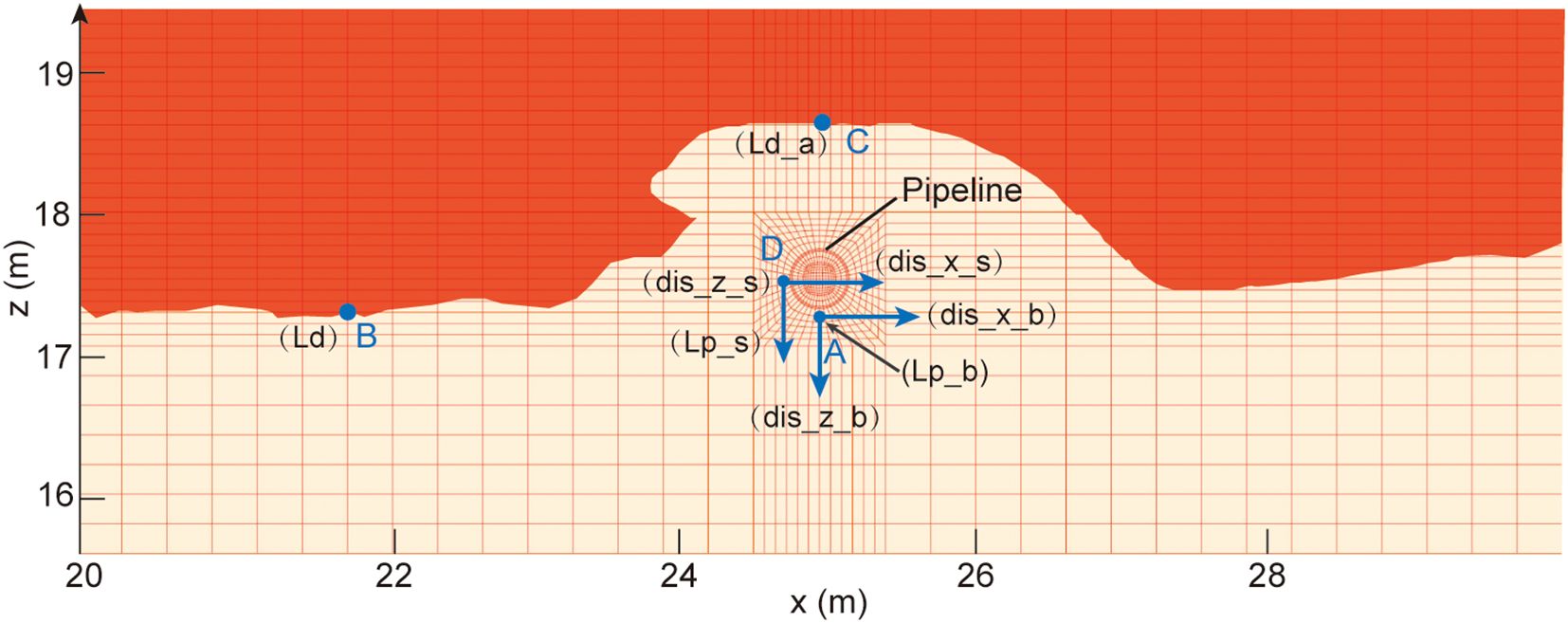
Figure 2. Definition of output parameters around the pipeline. The grid is the computational meshing for finite element computation, the blue dots are the four study points, and the parameters in parentheses are the output parameters of the monitoring points.
Point A: Located directly beneath the pipeline, used to analyze horizontal displacement (dis_x_b), vertical displacement (dis_z_b), and liquefaction potential (Lp_b) at this point.
Point B: Located away from the influence of the pipeline, used to determine the natural seabed liquefaction depth (Ld). This point helps in assessing the seabed’s own liquefaction depth without pipeline interference.
Point C: Located above the pipeline, used to assess the liquefaction depth above the pipeline (Ld_a). This point helps in understanding the impact of the pipeline on the liquefaction depth directly above it.
Point D: Located at the side of the pipeline, used to assess horizontal displacement (dis_x_s), vertical displacement (dis_z_s), and liquefaction potential (Lp_s) at this location.
By analyzing these four points, we can study the seabed’s liquefaction depth, pipeline displacements at different positions, liquefaction potentials, and the influence of the pipeline on seabed liquefaction. Points B and C are dynamic positions used to analyze the seabed liquefaction depth and the pipeline’s effect on liquefaction depth, providing two output parameters: Ld and Ld_a. Points A and D each have three output parameters, reflecting displacement and liquefaction tendency.
Table 2 presents the selected input variables critical for capturing hydrodynamic conditions and sediment characteristics, and the corresponding output parameters representing the seabed and pipeline responses.
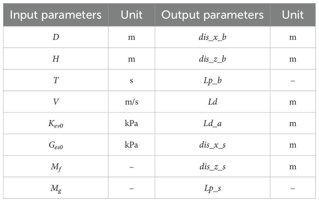
Table 2. Parameter settings of liquefaction of submarine pipeline and surrounding sediments under wave-current coupling.
Employing this dataset, generated through the application of the finite element method influenced by both waves and currents, represents a crucial advance in understanding seabed pipeline liquefaction under varied conditions. This strategy, integrated with machine learning modeling, sets the stage for more effective and expedient liquefaction disaster assessments in the study area. By concentrating on hydrodynamic conditions and sediment properties as input parameters, and displacement and liquefaction conditions as output parameters, our research is aligned with the requirements for a detailed comprehension of the mechanisms governing seabed and pipeline interactions under wave-current dynamics.
The dataset employed in this study covers all potential wave-current interactions for the area, including extremes of 100-year wave and current data to ensure that future conditions fall within the established parameter ranges. By incorporating detailed simulations at 2-meter depth intervals across potential liquefaction zones, our dataset maps all pertinent geological and hydrodynamic interactions. This coverage, derived from rigorous finite element analyses, not only guarantees the model’s high predictive accuracy for real-world scenarios but also justifies the extensive computational efforts involved, providing a solid foundation for applying machine learning techniques to predict seabed liquefaction effectively.
In our research, we used various machine learning (ML) models to analyze seabed pipeline liquefaction under wave-current interactions, concentrating on displacement and liquefaction outcomes. The adoption of ML models was based on their capacity to manage complex nonlinear relationships and exceptional predictive analytic prowess. Initially, six models including Random Forests (RF), Support Vector Machine (SVM), Gradient Boosting (GB), Multilayer Perceptron (MLP), K-Nearest Neighbors (KNN), and Extreme Gradient Boosting (XGBoost) were tested. After preliminary assessments, four models were chosen for their pattern recognition capabilities and predictive strengths, allowing a comprehensive evaluation of the dataset’s dynamics. The selection was based on comparative performance, where RF, SVM, GB, and MLP showed superior predictive accuracy and consistency, leading us to exclude KNN and XGBoost from further analysis.
While Convolutional Neural Networks (CNN) and Graph Neural Networks (GNN) are powerful deep learning models, they are particularly well-suited for data with spatial hierarchies (e.g., images) and graph-structured data, respectively. Our dataset consists of numerical simulation results represented as structured numerical features rather than images or graphs. Moreover, deep learning models like CNNs and GNNs typically require large amounts of data to train effectively, which may not be feasible with our dataset size. Therefore, we selected models that are better aligned with our data characteristics and research objectives.
Random Forests (RF), developed by Leo (2001), is an ensemble learning method that builds numerous decision trees at training time and outputs the mode of the classes (for classification) or the mean prediction (for regression) of the individual trees. The key idea is to construct multiple decision trees using bootstrap samples of the data and random subsets of features, then aggregate their predictions to improve generalization. By averaging predictions across multiple trees, each constructed on a random subset of the data and features, Random Forests mitigate the overfitting issues common to decision trees. This method enhances accuracy and robustness, particularly for datasets with complex structures and high dimensionality. In our study, RF is suitable due to its ability to handle nonlinear interactions between hydrodynamic parameters and seabed responses. Random Forests also handling missing values, maintain performance with significant data missing, and provide feature selection metrics. Despite its advantages, Random Forests can be computationally intensive and might underperform on unbalanced datasets without appropriate adjustments.
The Support Vector Machine (SVM), developed by Cortes and Vapnik (1995) at AT&T Bell Laboratories, is used for classification and regression tasks by identifying the optimal hyperplane that maximizes the margin between different classes or fits the data within a specified error margin. With the kernel trick, SVMs perform nonlinear classification by transforming the input space into a higher dimension where linear separation is possible. SVMs are particularly effective in high-dimensional spaces and are well-suited for applications like text classification and bioinformatics. In our research, SVM helps model the complex nonlinear relationships between input features and liquefaction outcomes. However, they require careful tuning of the kernel parameters and input feature scaling to prevent overfitting.
Gradient Boosting (GB), a technique developed by Jerome H. Friedman (2001), enhances the concept of boosting by sequentially combining weak learners to form a predictive model, with each new model addressing errors of its predecessors. This method, adaptable to various differentiable loss functions, is effectiveness in many predictive tasks. GB works by minimizing a loss function by adding weak learners that are fit to the negative gradient of the loss function. Gradient Boosting handles heterogeneous features and is robust against outliers in output spaces. In our study, GB is employed to capture the patterns and interactions in the dataset, improving prediction accuracy for seabed liquefaction. However, it demands careful tuning of parameters such as the number of stages, learning rate, and tree depth to avoid overfitting. It can be computationally demanding, especially with large datasets.
The Multilayer Perceptron (MLP) is a type of feedforward artificial neural network with layers including input, one or more hidden layers, and an output layer (David E et al., 1986). Nodes in each layer connect via weights to subsequent layers, enabling the network to capture complex relationships. MLPs employ nonlinear activation functions essential for modeling nonlinear phenomena and are recognized for their capability as universal function approximators, theoretically able to model any continuous function with adequate data. However, MLPs require significant computational resources and are sensitive to initial settings and architecture, with performance heavily reliant on network configuration.
To ensure the optimal performance of each machine learning model employed in this study, a hyperparameter tuning process was undertaken. As seen in Table 3, the key hyperparameters for each model were selected based on their influence on model performance. For Random Forests, important hyperparameters include the number of trees and the maximum depth of the trees, which control the ensemble size and complexity. In the Support Vector Machine model, the kernel type, regularization parameter (C), and gamma define the transformation of the input space and the trade-off between training error and model simplicity. Gradient Boosting’s performance is affected by the number of boosting stages, learning rate, and maximum depth of individual trees, which balance learning capacity and overfitting risk. For the Multilayer Perceptron, the architecture (number of layers and neurons), activation function, and learning rate are important for capturing patterns and ensuring convergence during training.
The chosen hyperparameters were validated through cross-validation techniques, evaluating their effectiveness in improving model accuracy and reducing overfitting. These tests involved running multiple simulations with different subsets of the data to ensure robustness across various scenarios. The final parameters were selected based on their performance in these tests, aiming to achieve the good generalization on unseen data while maintaining computational efficiency.
This approach to hyperparameter optimization has provided each model with a configuration for addressing the complex dynamics of wave-current interactions impacting seabed pipeline liquefaction, ensuring that the predictive models are both accurate and reliable.
As shown in Figure 3, the experimental steps are mainly divided into data pre-processing, model establish, and model evaluation.
Data pre-processing is an essential phase in machine learning, preparing raw data for effective modeling. This phase includes techniques such as normalization and dataset splitting to prepare the data for modeling. These steps are pivotal for addressing scale disparities among features and evaluating model performance on new data, ensuring the efficacy and generalizability of our machine learning applications.
Normalization, or feature scaling, is crucial for standardizing the range of independent variables or features within the data. This step is vital because scale disparities can cause some algorithms to weigh larger values more heavily. To address this, we apply Min-Max Scaling, which adjusts features to a uniform scale. By rescaling the data typically between [0, 1] or [-1, 1], we ensure each feature equally influences the model’s predictions, enhancing the training process and comparability across different features.
Following normalization, we split the dataset into training and testing sets to train the models and assess their predictive capabilities on unseen data. Specifically, we allocated 80% of the dataset for training and 20% for testing. This split allows us to evaluate how well the models generalize to new data not used during the training process. By assessing the models’ performance on the independent test set, we can ensure that our conclusions about model effectiveness are based on their ability to predict new cases accurately.
Correlation analysis helps us understand the interrelations among different parameters within our dataset. We employ the Pearson correlation coefficient to quantify the linear relationships between each variable pair. We aggregate these coefficients and display them in a heatmap (Figure 4) to identify significant predictors for our models.
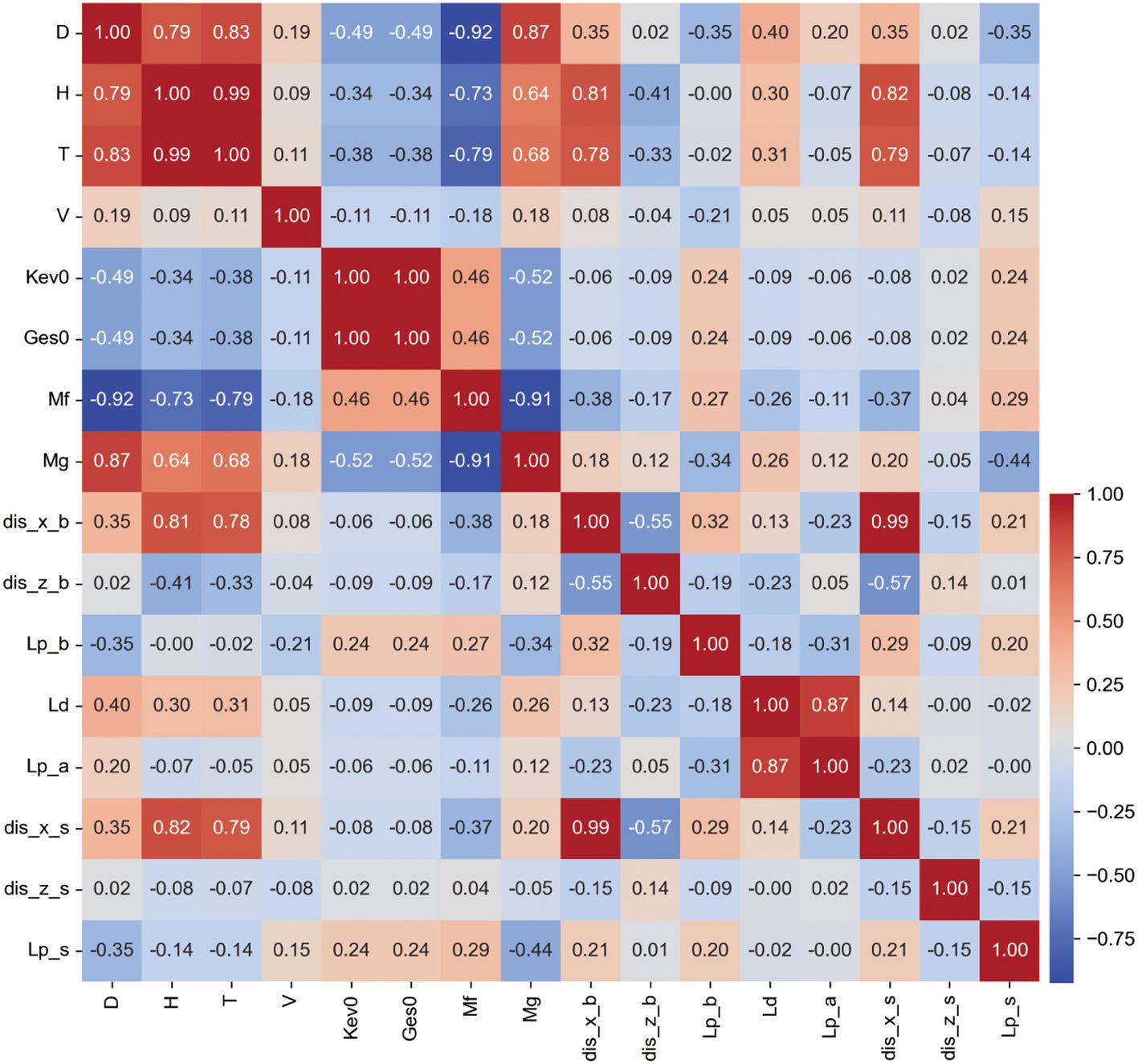
Figure 4. Correlation coefficient heatmap. Colors closer to red indicate stronger positive correlation between parameters, colors closer to blue indicate stronger negative correlation, and colors closer to white indicate weaker correlation.
Our findings indicate that wave height (H), wave period (T), and water depth (D) are highly correlated with the output parameters, with sum of correlation coefficients of 2.627, 2.484, and 2.029 respectively, highlighting their importance in predicting seabed pipeline and sediment liquefaction. Conversely, parameters such as sediment friction angle (Mf) and sediment cohesion (Mg) show moderate correlations, with sums of 1.871 and 1.714, indicating a less dominant impact compared to primary hydrodynamic factors. The bulk modulus (Kev0), shear modulus (Ges0), and flow velocity (V) exhibit the lowest correlations, with sums of 0.882, 0.882, and 0.757 respectively, suggesting a minor influence on the outputs in this study’s context.
To ensure input parameters are not only statistically significant but also physically meaningful, we organize them into three computational scenarios: (1) using all eight parameters to maximize informational breadth; (2) using H, T, D, Mf, Mg, and V to incorporate all hydrodynamic factors with the highest correlating sediment parameters; and (3) selecting H, T, D, and V, focusing on core hydrodynamic parameters. This tiered approach allows thoroughly explore data, maintaining both statistical relevance and physical comprehensiveness, supporting the analysis of hydrodynamic impacts on seabed pipeline and sediment liquefaction. It enables us to develop robust, insightful predictive models.
In our study, cross-validation plays a pivotal role in refining the performance and reliability of all employed models, including SVM, Random Forests, Gradient Boosting, and MLP. This method verifies the effectiveness of machine learning models by dividing the dataset into multiple folds. Each fold is sequentially used for validation while the remaining serve as training data. This process ensures that every segment of the dataset is used for both training and validation, thereby enhancing the model’s ability to generalize to new, unseen data. Cross-validation is essential for fine-tuning model parameters, boosting their performance and ensuring an unbiased evaluation of their predictive accuracy.
Building upon the insights gained from our correlation analysis, we utilize four machine learning models: Random Forests, SVM, Gradient Boosting, and MLP. Each model is trained across three sets of input parameters, designed to maximize the extraction of relevant insights from our dataset. This includes using all eight parameters, a focus on key hydrodynamic factors with highly correlated sediment parameters, and a strategy concentrating on essential hydrodynamic factors. This structured variation in parameter utilization is designed to assess the potential of our dataset in predicting seabed dynamics under varying conditions.
By systematically training each model with these diverse input setups, we aim to uncover the specific impacts of different parameter emphases on the prediction of pipeline displacement, seabed liquefaction, and adjacent liquefaction phenomena caused by wave-current interactions. This comprehensive training approach not only elucidates the strengths and flexibility of each model but also enhances the trustworthiness of their predictions across various scenarios, thereby ensuring a thorough evaluation of seabed and pipeline behaviors in response to hydrodynamic forces.
For evaluating the four models’ accuracy in predicting wave-induced liquefaction, we employ Mean Squared Error (MSE) and Mean Absolute Error (MAE) as our primary metrics. These indicators quantify the average discrepancies between the predicted values and the actual outcomes. MSE is particularly valuable for its sensitivity to larger errors, making it crucial in scenarios where such errors are less tolerable, while MAE provides a straightforward average error magnitude, offering an intuitive gauge of prediction accuracy without unduly emphasizing larger mistakes. The choice of these metrics ensures a balanced assessment of model performance, highlighting not just the average accuracy but also how the models handle more extreme cases, which are critical in understanding and mitigating the risks associated with seabed instability.
All finite element simulations using the FSSI-CAS model and the machine learning computations were performed on the same workstation to ensure consistency in computational time comparisons. The computations were executed on a high-performance Dell 3660 workstation equipped with an Intel Core i9-12900K CPU, 128 GB of RAM, and an NVIDIA RTX 4090 GPU, providing the necessary computational power to efficiently handle intensive numerical simulations and machine learning tasks. The machine learning models were implemented using scikit-learn, a widely used Python library renowned for its comprehensive tools for machine learning and statistical modeling. This setup provided a robust platform for both the intensive numerical simulations and the efficient training and execution of the machine learning models.
To evaluate the accuracy of various machine learning models in predicting wave-induced liquefaction, this study used a dual approach: direct visual comparisons between actual and predicted values, and a detailed statistical analysis. Figure 5 illustrates the discrepancies in predictions across four machine learning models for eight distinct output parameters, offering a comprehensive view of the prediction performance. Notably, the Multi-Layer Perceptron (MLP) model demonstrated the lowest accuracy across all parameters, underscoring its limitations in addressing the specific challenges of wave-induced liquefaction prediction. On the other hand, the Random Forest (RF) model displayed consistent predictions, though it exhibited slight deficiencies in accurately predicting the liquefaction potential (Lp_b).
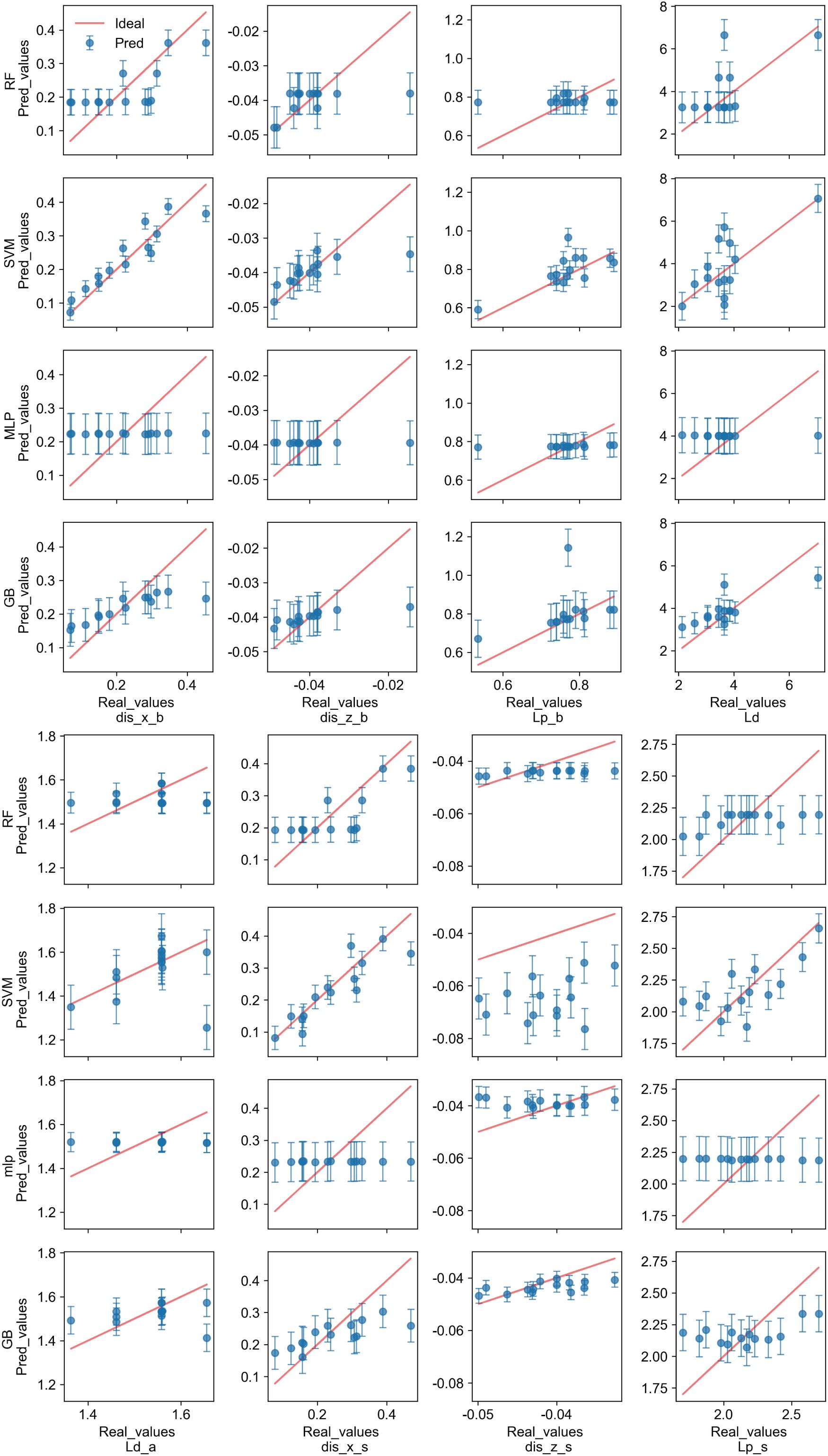
Figure 5. Comparison of output results of different machine learning models with actual results. The red line represents the ideal relationship between the true and predicted values, indicating the target prediction, with points closer to the line reflecting better prediction performance.
The Support Vector Machine (SVM) and Gradient Boosting (GB) models generally provided predictions that were closely aligned with actual values, indicative of their higher accuracy. However, the SVM model encountered significant discrepancies specifically in predicting the z-direction displacement beside the pipeline (dis_z_s), deviating markedly from the ideal prediction trajectory. Conversely, the GB model, despite some parameters not fitting as accurately as those of the SVM, presented smaller overall prediction errors and consistently delivered more precise predictions across all eight output parameters.
To ensure the stability of the models and conduct a comprehensive evaluation, each model was run 20 times independently with different random seeds. This approach allowed us to assess the performance of each model under varied initial conditions, thereby enhancing the reliability of the results. Figure 6 presents the normalized statistical data on prediction accuracy, where the Gradient Boosting (GB) model exhibited a compact distribution across Mean Squared Error (MSE), Mean Absolute Error (MAE), and the newly included metrics of Root Mean Squared Error (RMSE) and R-squared (R2). This compact distribution suggests minimal predictive errors and enhanced performance consistency. The Random Forest (RF) model showed a slightly broader distribution, particularly in RMSE and R2, indicating some variability in its predictions. In contrast, the distribution for the Multi-Layer Perceptron (MLP) model was notably wider, reflecting lower precision and higher variability in performance. The RF and Support Vector Machine (SVM) models demonstrated moderate accuracy levels, with the RF model showing higher MAE and RMSE in the upper quartile, indicating potential discrepancies in certain predictions. While the SVM model maintained a lower median in MAE and RMSE, suggesting generally superior precision, its higher R2 values in the upper quartile hinted at significant errors under complex scenarios, especially in cases where R2 was negative.
Table 4 summarizes these findings by summarizing the statistical indicators for each model. The GB model consistently outperformed the others, as highlighted by the bolded values, which represent the best performance in each category. Specifically, the GB model achieved the lowest maximum and average MSE and MAE, reinforcing its superior predictive accuracy and stability across the test cases. The SVM model, while showing a strong performance in terms of the minimum MSE and MAE, struggled with the R2 metric, particularly evidenced by negative values in complex scenarios, which reflects its occasional instability. The MLP model, although useful, exhibited the widest range in error metrics, indicating a higher degree of variability and lower reliability in predictions.
In this evaluation, with the inclusion of RMSE and R2 as additional performance metrics, the GB model consistently demonstrated the highest predictive accuracy, particularly excelling in MSE and MAE. The SVM model also performed well in terms of MAE and RMSE, but the occurrence of negative R2 values indicates potential stability issues in certain scenarios. The RF model, while showing competitive results, exhibited a broader range of errors, especially in the upper quartiles of RMSE and MAE, indicating variability in specific predictions. Overall, the GB model remains the most effective across various metrics, with the SVM model following closely behind, though with less stability under complex conditions.
This section delves into the predictive accuracies concerning the liquefaction of submarine pipelines and adjacent sediments under the effects of wave-current interactions. Through analysis using normalized Mean Absolute Error (MAE) and Mean Squared Error (MSE) heatmaps (Figure 7) and detailed bar charts (Figure 8), we categorized the prediction errors across various output parameters into three principal groups.
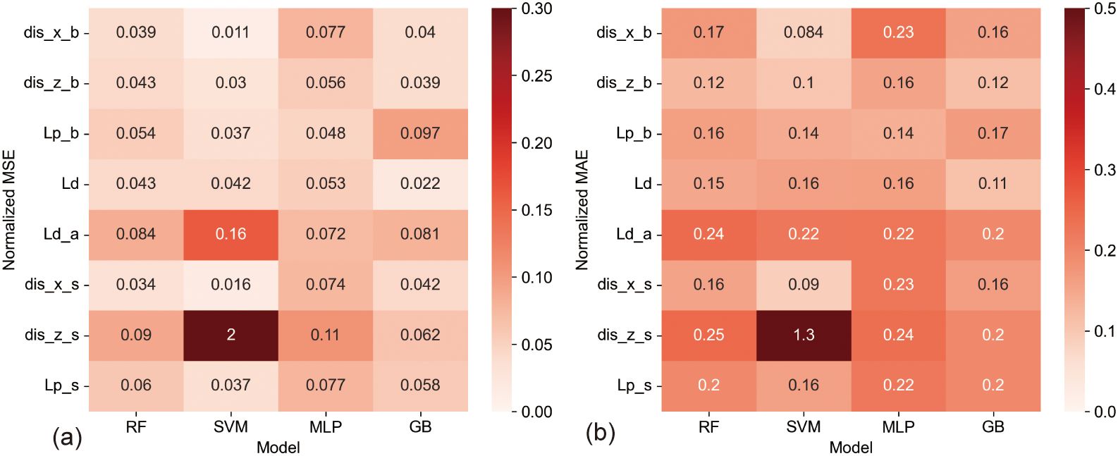
Figure 7. The normalized MSE and MAE heatmaps between different models for output parameters. (A) is the normalized MSE, and (B) is the normalized MAE.
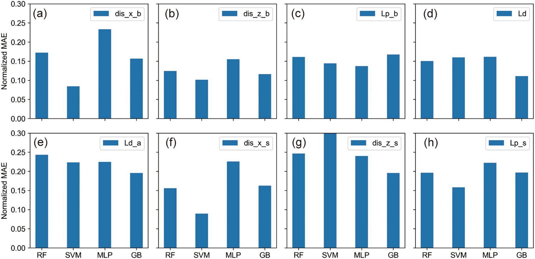
Figure 8. The MAE bar charts for different output parameters. (A–H) correspond to the eight different output parameters.
The first group consists of parameters that demonstrated minimal predictive errors: the z-direction displacement beneath the pipeline (dis_z_b), the liquefaction potential beneath the pipeline (Lp_b), and the seabed liquefaction depth (Ld). For these parameters, normalized MAE values were typically below 0.2, suggesting a high level of accuracy in model predictions. The second group encompasses parameters with moderate predictive challenges, including the x-direction displacement beneath the pipeline (dis_x_b), the x-direction displacement beside the pipeline (dis_x_s), and the liquefaction potential beside the pipeline (Lp_s). Here, some models showed normalized MAE values exceeding 0.2, indicating increased difficulty in accurate predictions.
The third group featured the most significant predictive errors, particularly for the liquefaction depth above the pipeline (Ld_a) and the z-direction displacement beside the pipeline (dis_z_s), where normalized MAE values generally surpassed 0.2. Notably, the SVM model exhibited a particularly high MAE when predicting the z-direction displacement beside the pipeline (dis_z_s), underscoring the substantial challenges involved in forecasting these parameters.
These variations in predictive accuracy underscore the differing dynamic responses of the seabed and pipeline environment under hydrodynamic influences. Specifically, the area beneath the pipeline is characterized by more stable and less complex physical processes, which typically results in lower predictive errors. Conversely, the pipeline’s lateral regions, heavily influenced by dynamic hydrodynamic factors, exhibit more complex changes, making accurate predictions more challenging. Moreover, the liquefaction depth above the pipeline (Ld_a) shows higher prediction difficulties compared to the more distal seabed liquefaction depth (Ld), likely due to the direct impacts affecting the area above the pipeline. This reflects the inherent complexity and variability of liquefaction phenomena close to submarine infrastructures.
In examining the effects of different input parameter combinations on prediction accuracy, this analysis focuses on the Gradient Boosting (GB) model within three distinct scenarios: the first incorporating all eight parameters, the second utilizing six parameters emphasizing hydrodynamic factors alongside highly correlated sediment characteristics, and the third limited to four core hydrodynamic parameters.
Insights drawn from Figure 9’s boxplots indicate closely aligned median and interquartile ranges for the MSE across the three configurations of the GB model, suggesting a negligible difference in overall prediction performance. However, the MAE metrics present a nuanced picture: GB1 showcases a lower median yet a higher upper quartile, indicative of generally superior performance but interspersed with notable errors. Conversely, GB3 exhibits the highest upper limit in MAE, highlighting possible prediction inconsistencies under certain conditions.
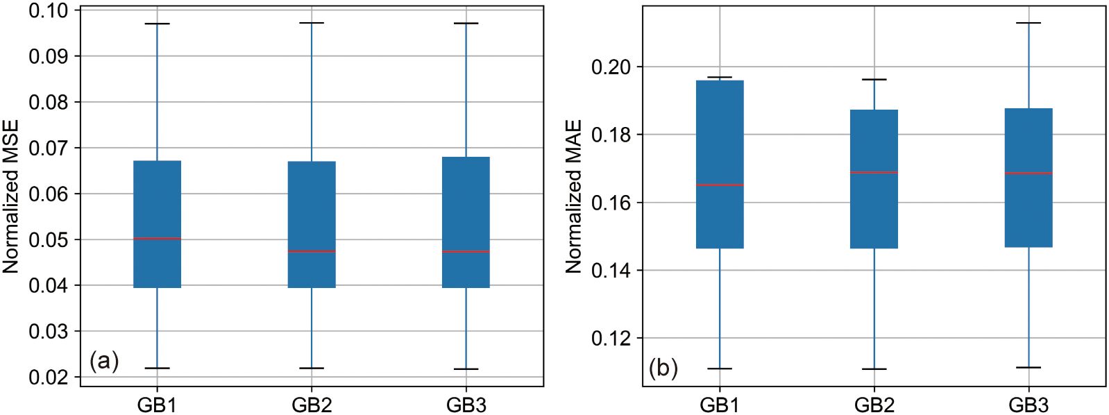
Figure 9. Normalized prediction accuracy of GB models with different input parameters. (A) Boxplot of Normalized MSE for GB1, GB2, and GB3 models. (B) Boxplot of Normalized MAE for GB1, GB2, and GB3 models.
A granular analysis provided in Figure 10 assesses the predictive performance for each output parameter. For parameters such as dis_x_b, dis_z_b, Lp_b, and Ld, all three GB model configurations demonstrated comparable accuracy levels in both MSE and MAE metrics. The rest of the parameters displayed slight discrepancies, with GB2 marginally outshining both GB1 and GB3. Observations from Figure 11 further corroborate these findings, showing similar error distributions across the models, with GB2 generally surpassing GB1 and GB3 in terms of overall predictive accuracy.
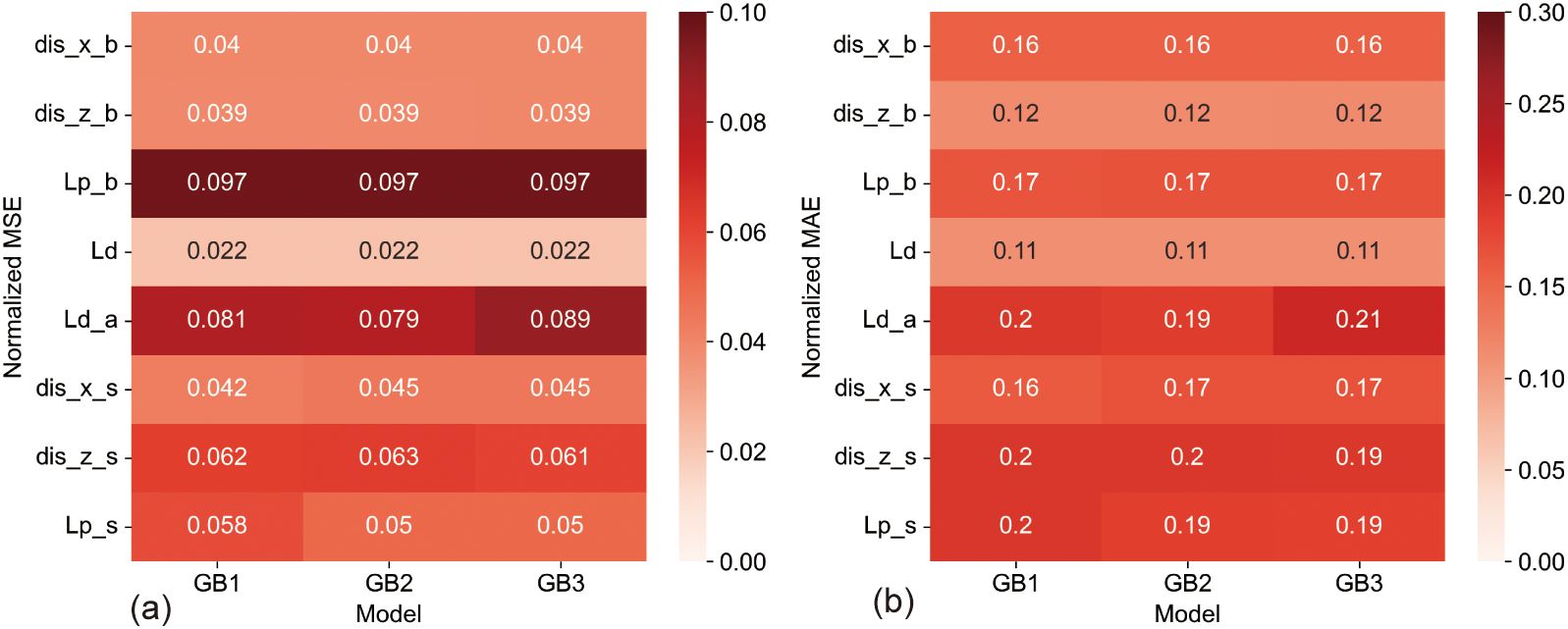
Figure 10. Comparative Heatmaps of Prediction Errors for GB Models, (A) Heatmap of Normalized MSE showing the distribution of prediction errors for GB1, GB2, and GB3 across the different output parameters. (B) Heatmap of Normalized MAE illustrating the error consistency and outliers for each GB model variant in relation to the output parameters.
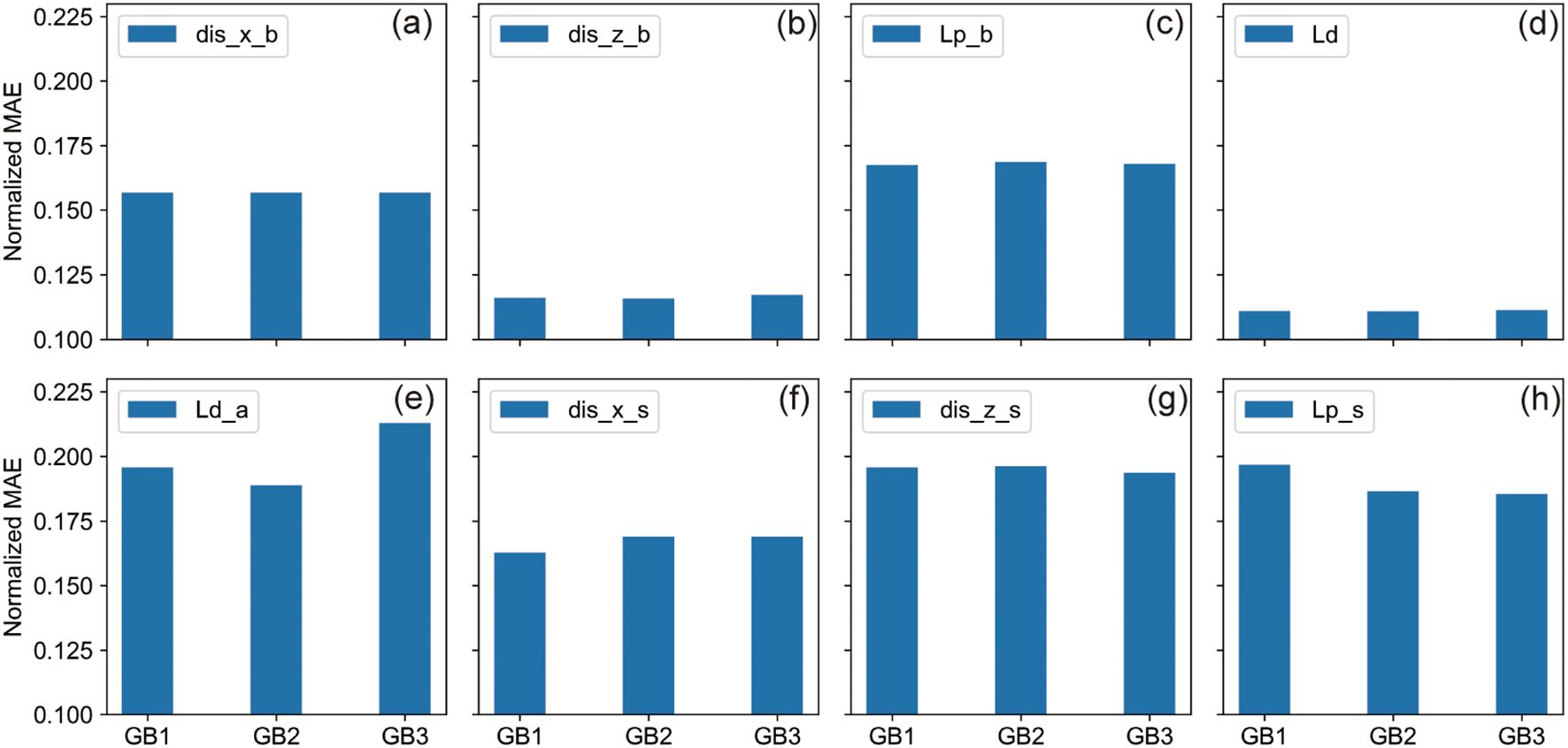
Figure 11. The Bar Charts of Predictive Performance Across Output Parameters for GB Models. (A–H) Bar charts representing the Normalized MSE and MAE for each output parameter, respectively, across the three GB model scenarios, displaying the comparative analysis of prediction errors: (A) dis_x_b, (B) dis_z_b, (C) Lp_b, (D) Ld, (E) Ld_a, (F) dis_x_s, (G) dis_z_s, and (H) Lp_s.
The experimental setup entailed distinct groups: the first exploited all eight parameters, the second omitted two sediment parameters of lower correlation, retaining six, while the third was restricted to just four hydrodynamic parameters. Ultimately, each group’s modeling yielded fairly consistent predictions, with no significant discrepancies observed. The modest superiority of GB2 over GB1 could be attributed to the exclusion of two lesser-correlated sediment parameters, which ostensibly streamlined the model’s fitting and predictive accuracy. Despite omitting all sediment-related factors, GB3 maintained commendable accuracy, likely due to the sediment characteristics in the study area - predominantly silt - exhibiting only minor variations. Collectively, all input configurations achieved satisfactory prediction accuracy, with the models including both hydrodynamic and sediment parameters, particularly GB1 and GB2, demonstrating enhanced precision. Nonetheless, for computational efficiency, models employing only key hydrodynamic parameters-depth, wave height, and current—may suffice for effective training and prediction.
This discussion elaborates on the comparative performance of different machine learning models as presented in the results section, focusing on their efficacy in addressing wave-induced liquefaction and the influence of varied input parameters. The Gradient Boosting (GB) and Support Vector Machine (SVM) models emerged as superior in most tested scenarios, attributable to their inherent mathematical frameworks and suitability for the complexities of wave-induced liquefaction phenomena. The GB model, with its robust nonlinear modeling abilities and efficient gradient boosting processes, is particularly effective in tackling intricate geological challenges. In contrast, the SVM model, which strategically optimizes category margins to maximize inter-class distance, excels in scenarios with well-defined physical boundaries such as those presented by wave-induced phenomena.
However, challenges persist with other models; the Multilayer Perceptron (MLP), due to its deep learning architecture, is prone to overfitting unless adequately tuned, which can diminish its predictive accuracy. The Random Forest (RF) model, typically reliable in both classification and regression settings, did not reach its full potential in this study’s specific scenarios, likely due to its inherent randomness and sensitivity to data anomalies.
Deeper investigation into the models’ performance across various parameters indicates that straightforward geological contexts, like the seabed liquefaction depth (Ld), allow most models to predict with reasonable accuracy. This success underscores the models’ capability to effectively capture essential dynamics when geological influences are less complex. In contrast, the areas adjacent to pipelines, significantly influenced by dynamic hydrodynamic forces, present a greater challenge, exhibiting more intricate geological behaviors and subsequently, lower predictive accuracies, particularly for parameters like the liquefaction potential beside the pipeline (Lp_s).
The computational efficiency of the machine learning models presents a significant advantage over the traditional finite element method. Specifically, the FSSI-CAS finite element simulations required approximately 5 hours per data point to compute the seabed liquefaction around the buried pipeline, amounting to a total of over 70 hours for all 14 data points on the Intel Core i9-12900K workstation. In contrast, the trained machine learning models, including the Gradient Boosting model, generated predictions for all 14 data points in seconds on the same hardware configuration. This dramatic reduction in computational time underscores the practicality of the machine learning approach for real-time predictions and large-scale simulations, facilitating more efficient engineering analyses and decision-making processes.
The complexities observed near the pipeline, exacerbated by the interactive effects of waves and currents, make these areas particularly difficult to model accurately. These findings highlight the nuanced requirements of predictive models under variable geological conditions and emphasize the necessity of selecting appropriate machine learning strategies that align with the specific nature of the geological phenomena under study.
In this study, we utilized four machine learning models to predict wave-induced liquefaction and observed notable achievements. Although these models are widely recognized within the machine learning community, the extensive variety of available methodologies suggests that alternative models could potentially yield better outcomes for specific challenges. This insight drives our intention to explore a wider array of machine learning models in future research to pinpoint the optimal approach for distinct scenarios.
Regarding the dataset used for wave-induced liquefaction studies, current limitations are evident. The existing data primarily addresses the static relationship between input and final state parameters without incorporating time-series data that capture the sediment dynamics over time. To enhance our predictive accuracy and model the dynamic process of wave-induced liquefaction more effectively, we plan to develop a comprehensive dynamic dataset that includes temporal dimensions. Future efforts will include experimenting with the integration of Recurrent Neural Networks (RNNs) and Gradient Boosting (GB) models, exploiting their strengths in processing time-series data to refine our predictions.
Additionally, the application of machine learning to predict wave-induced liquefaction significantly enhances time efficiency. Machine learning methods can achieve results comparable to those of traditional finite element numerical approaches but in a fraction of the time, offering a substantial advantage for the rapid assessment and forecasting of marine disasters. Our future work will focus on further refining these models to improve both their efficiency and accuracy in disaster prediction scenarios.
Overall, despite the progress made, opportunities remain for advancements in model selection, dataset enhancement, and the application of models. We are committed to ongoing research and innovation to more effectively harness machine learning for the prediction of wave-induced liquefaction and other complex marine geological challenges, aiming to bolster marine engineering safety with robust technological support.
This study conducted a detailed comparison of the predictive effectiveness of four classic machine learning models on the complex issue of wave-current-pipeline-liquefaction interactions, examining the predictive accuracy of different models, the impact of various input parameters on prediction accuracy, and the accuracy levels of different output parameters. Through this process, we have deepened our understanding of the performance of each model in predicting geological disasters and unveiled the potential and challenges of applying machine learning in marine geological engineering predictions. The main conclusions are as follows:
(1) Model Performance Comparison: The GB and SVM models demonstrated higher predictive accuracy in most test scenarios. The GB model provided stable and accurate predictions across all output parameters, while the SVM model showed inaccuracies in predicting certain parameters but was highly accurate for others. Overall, the GB model is characterized by its stability, powerful nonlinear fitting capabilities, and efficiency in processing complex geological data.
(2) Impact of Input Parameters: The combination of different input parameters significantly affects model predictive accuracy. Reducing parameters with low correlation in sediment characteristics led to lower prediction errors. Retaining only hydrodynamic parameters increased errors but within an acceptable range, highlighting the importance of selecting appropriate input parameters to improve prediction accuracy.
(3) Importance of Rapid Prediction: Compared to traditional finite element numerical methods, using machine learning models for wave-induced liquefaction predictions can significantly reduce computation time, providing a powerful tool for rapid disaster assessment and early warning in marine engineering. This capability to rapidly predict is crucial for enhancing the safety and response efficiency of marine engineering projects.
(4) Dataset Construction and Limitations: Despite the progress made, this study underscores the need for comprehensive dataset development, particularly the inclusion of time-series data to capture the dynamics of wave-induced liquefaction. Future efforts should focus on enriching datasets with temporal dimensions to enhance model accuracy and generalization, addressing a critical gap in current research methodologies.
Publicly available datasets were analyzed in this study. This data can be found here: https://doi.org/10.5281/zenodo.11910960.
XD: Writing – review & editing, Writing – original draft, Resources, Methodology, Funding acquisition, Data curation, Conceptualization. YS: Writing – review & editing, Resources. DW: Writing – review & editing, Methodology. KH: Writing – review & editing, Resources. WC: Writing – review & editing. ZX: Writing – review & editing, Validation. XZ: Writing – review & editing.
The author(s) declare that financial support was received for the research, authorship, and/or publication of this article. The authors are grateful to the funding support from The National Natural Science Foundation of China under contract NO. 42102326; the Basic Scientific Fund for National Public Research Institutes of China under contract NO. 2022Q05; National Key R&D Program of China (Grant No.2022YFC2803800); The National Natural Science Foundation of China under contract NO. 41876066.
The authors would like to thank to the developers who proposed the Pytorch deep learning package (https://pytorch.org/), which support the CNN modeling in this paper.
The authors declare that the research was conducted in the absence of any commercial or financial relationships that could be construed as a potential conflict of interest.
All claims expressed in this article are solely those of the authors and do not necessarily represent those of their affiliated organizations, or those of the publisher, the editors and the reviewers. Any product that may be evaluated in this article, or claim that may be made by its manufacturer, is not guaranteed or endorsed by the publisher.
Chen H., Zhang J., Tong L., Sun K., Guo Y., Wei C. (2023). Experimental study of soil responses around a pipeline in a sandy seabed under wave-current load. Appl. Ocean Res. 130, 103409. doi: 10.1016/j.apor.2022.103409
Cheng A. H.-D., Liu P. L.-F. (1986). Seepage force on a pipeline buried in a poroelastic seabed under wave loadings. Appl. Ocean Res. 8, 22–32. doi: 10.1016/S0141-1187(86)80027-X
Cortes C., Vapnik V. (1995). Support-vector networks. Mach. Learn 20, 273–297. doi: 10.1007/BF00994018
David E R., Geoffrey H., Ronald J. (1986). Learning representations by back-propagating errors. Nature 323, 533–536. doi: 10.1038/323533a0
Du X. (2024). A novel strategy for fast liquefaction detection around marine pipelines:A finite element-machine learning approach. doi: 10.5281/zenodo.11910960
Du X., Sun Y., Song Y., Dong L., Zhao X. (2023a). Revealing the potential of deep learning for detecting submarine pipelines in side-scan sonar images: an investigation of pre-training datasets. Remote Sens. 15, 4873. doi: 10.3390/rs15194873
Du X., Sun Y., Song Y., Sun H., Yang L. (2023b). A comparative study of different CNN models and transfer learning effect for underwater object classification in side-scan sonar images. Remote Sens. 15, 593. doi: 10.3390/rs15030593
Du X., Sun Y., Song Y., Xiu Z., Su Z. (2022). Submarine landslide susceptibility and spatial distribution using different unsupervised machine learning models. Appl. Sci. 12, 10544. doi: 10.3390/app122010544
Du X., Sun Y., Song Y., Yu Y., Zhou Q. (2023c). Neural network models for seabed stability: a deep learning approach to wave-induced pore pressure prediction. Front. Mar. Sci. 10. doi: 10.3389/fmars.2023.1322534
Friedman J. H. (2001). Greedy function approximation: A gradient boosting machine. Ann. Statist. 29, 1189–1232. doi: 10.1214/aos/1013203451
Gao F. P., Jeng D. S., Sekiguchi H. (2003). Numerical study on the interaction between non-linear wave, buried pipeline and non-homogenous porous seabed. Comput. Geotech. 30, 535–547. doi: 10.1016/S0266-352X(03)00053-3
Guo X., Nian T., Zhao W., Gu Z., Liu C., Liu X., et al. (2022). Centrifuge experiment on the penetration test for evaluating undrained strength of deep-sea surface soils. Int. J. Min. Sci. Technol. 32, 363–373. doi: 10.1016/j.ijmst.2021.12.005
He K., Ye J. (2023). Dynamics of offshore wind turbine-seabed foundation under hydrodynamic and aerodynamic loads: A coupled numerical way. Renewable Energy 202, 453–469. doi: 10.1016/j.renene.2022.11.029
Hsu T.-J., Sakakiyama T., Liu P. L.-F. (2002). A numerical model for wave motions and turbulence flows in front of a composite breakwater. Coast. Eng. 46, 25–50. doi: 10.1016/S0378-3839(02)00045-5
Jeng D. S. (2001). Numerical modeling for wave–seabed–pipe interaction in a non-homogeneous porous seabed. Soil Dynamics Earthquake Eng. 21, 699–712. doi: 10.1016/S0267-7261(01)00043-4
Jeng D.-S., Cheng L. (2000). Wave-induced seabed instability around a buried pipeline in a poro-elastic seabed. Ocean Eng. 27, 127–146. doi: 10.1016/S0029-8018(98)00046-8
Jeng D.-S., Seymour B. R., Li J. (2007). A new approximation for pore pressure accumulation in marine sediment due to water waves. Int. J. Numeric. Anal. Methods Geomech. 31, 53–69. doi: 10.1002/nag.547
Kiziloz B., Çevik E., Yüksel Y. (2013). Scour below submarine pipelines under irregular wave attack. Coast. Eng. 79, 1–8. doi: 10.1016/j.coastaleng.2013.04.001
Larsen B. E., Fuhrman D. R., Sumer B. M. (2016). Simulation of wave-plus-current scour beneath submarine pipelines. J. Waterway Port Coastal Ocean Eng. 142, 04016003. doi: 10.1061/(ASCE)WW.1943-5460.0000338
Madsen S. (1978). Wave-induced pore pressures and effective stresses in a porous bed. Geotechnique 28, 377–394. doi: 10.1680/geot.1978.28.4.377
Magda W. (1997). Wave-induced uplift force on a submarine pipeline buried in a compressible seabed. Ocean Eng. 24, 551–576. doi: 10.1016/S0029-8018(96)00031-5
Martin P. P., Bolton Seed H. (1983). One-dimensional dynamic ground response analyses: J geotech engng div ASCE, V108, NGT7, July 1982, P935–952. Int. J. Rock Mech. Min. Sci. Geomech. Abstr. 20, A9. doi: 10.1016/0148-9062(83)91690-X
Rateria G., Maurer B. W. (2022). Evaluation and updating of Ishihara’s, (1985) model for liquefaction surface expression, with insights from machine and deep learning. Soils Found. 62, 101131. doi: 10.1016/j.sandf.2022.101131
Seed H. B., Rahman M. S. (1978). Wave-induced pore pressure in relation to ocean floor stability of cohesionless soils. Mar. Geotechnol. 3, 123–150. doi: 10.1080/10641197809379798
Sumer B. M. (2014). Advances in seabed liquefaction and its implications for marine structures. Geotechnical Engineering. 45, 1-14.
Wang X., Jeng D. S., Lin Y. S. (2000). Effects of a cover layer on wave-induced pore pressure around a buried pipe in an anisotropic seabed. Ocean Eng. 27, 823–839. doi: 10.1016/S0029-8018(99)00012-8
Ye J., He K. (2021). Dynamics of a pipeline buried in loosely deposited seabed to nonlinear wave & current. Ocean Eng. 232, 109127. doi: 10.1016/j.oceaneng.2021.109127
Ye J., Jeng D., Wang R., Zhu C. (2015). Numerical simulation of the wave-induced dynamic response of poro-elastoplastic seabed foundations and a composite breakwater. Appl. Math. Model. 39, 322–347. doi: 10.1016/j.apm.2014.05.031
Ye J., Lu Q. (2022). Seismic dynamics of a pipeline shallowly buried in loosely deposited seabed foundation. Ocean Eng. 243, 110194. doi: 10.1016/j.oceaneng.2021.110194
Zhou X.-L., Jeng D.-S., Yan Y.-G., Wang J.-H. (2013). Wave-induced multi-layered seabed response around a buried pipeline. Ocean Eng. 72, 195–208. doi: 10.1016/j.oceaneng.2013.06.031
Keywords: submarine pipelines, gradient boosting, support vector machine, machine learning, wave-current coupling
Citation: Du X, Song Y, Wang D, He K, Chi W, Xiu Z and Zhao X (2024) Comparative evaluation of machine learning models for assessment of seabed liquefaction using finite element data. Front. Mar. Sci. 11:1491899. doi: 10.3389/fmars.2024.1491899
Received: 05 September 2024; Accepted: 23 October 2024;
Published: 15 November 2024.
Edited by:
Charlotte Lyddon, University of Liverpool, United KingdomReviewed by:
Andrés Payo, The Lyell Centre, United KingdomCopyright © 2024 Du, Song, Wang, He, Chi, Xiu and Zhao. This is an open-access article distributed under the terms of the Creative Commons Attribution License (CC BY). The use, distribution or reproduction in other forums is permitted, provided the original author(s) and the copyright owner(s) are credited and that the original publication in this journal is cited, in accordance with accepted academic practice. No use, distribution or reproduction is permitted which does not comply with these terms.
*Correspondence: Yupeng Song, c29uZ3l1cGVuZ0BmaW8ub3JnLmNu; Dong Wang, ZG9uZ3dhbmdAb3VjLmVkdS5jbg==
Disclaimer: All claims expressed in this article are solely those of the authors and do not necessarily represent those of their affiliated organizations, or those of the publisher, the editors and the reviewers. Any product that may be evaluated in this article or claim that may be made by its manufacturer is not guaranteed or endorsed by the publisher.
Research integrity at Frontiers

Learn more about the work of our research integrity team to safeguard the quality of each article we publish.