Data mining-based machine learning methods for improving hydrological data: a case study of salinity field in the Western Arctic Ocean

The Beaufort Gyre is the largest freshwater reservoir in the Arctic Ocean. Long-term changes in freshwater reservoirs are critical for understanding the Arctic Ocean, and data from various sources, particularly observation or reanalysis data, must be used to the greatest extent possible. Over the past two decades, a large number of intensive field observations and ship surveys have been conducted in the western Arctic Ocean to obtain a large amount of CTD (Conductivity, Temperature, and Depth) data. Multi-machine learning methods were assessed and merged to reconstruct the annual salinity product in the Western Arctic Ocean over the period 2003-2022. Data mining-based machine learning methods reconstructed salinity product based on input variables determined by physical processes, such as sea level pressure, bathymetry, sea ice concentration, and sea ice drift. The root-mean-square error of sea surface salinity, in comparison to deep water, was effectively managed during machine learning, which exhibits higher sensitivity to variations in the atmosphere, sea ice, and ocean. The mean absolute errors in freshwater content and halocline depth within the Beaufort Gyre region for the salinity product from 2003 to 2022 are 0.98 m and 1.31 m, respectively, when compared to observational data. The salinity product provides reliable characterizations of freshwater content in the Beaufort Gyre and its variations at halocline depth. In polar regions where lacking observed data, we can build data mining-based machine learning methods to generate reliable data products to compensate for the inconvenience. Furthermore, the application potential of this multi-machine learning results approach for evaluating and integrating extends beyond the salinity field, encompassing hydrometeorology, sea ice thickness, polar biogeochemistry, and other related fields.

1 Introduction

In contrast to the low- and mid-latitude oceans, the Arctic Ocean is characterized by its extensive sea ice coverage and near-freezing sea surface water. Variations in salinity in the Western Arctic Ocean have profound implications for stratification strength, ocean circulation patterns, and biogeochemical cycles (Carmack et al., 2016; Cornish et al., 2020). Freshwater reservoirs and its evolution, which are closely related to the change of seawater salinity, have become the focus of research in the Arctic Ocean. Consequently, acquiring precise salinity data is of paramount importance for enhancing our understanding of this distinctive oceanic environment. The wind-driven surface circulation in the Arctic Ocean is primarily governed by two key factors: the anti-cyclonic Beaufort Gyre and the Transpolar Drift. Moreover, substantial quantities of freshwater accumulate in the Beaufort Gyre in the Western Arctic Ocean. The release of the freshwater exerts a significant impact on local climate dynamics as well as global climate change at large scales (Carmack et al., 2008; Giles et al., 2012; Proshutinsky et al., 2009, 2019).

The Western Arctic Ocean (140°E-120°W, 68°N-90°N) spans a vast territory with the Beaufort Gyre, the largest freshwater reservoir in the Arctic Ocean (Figure 1). In the Western Arctic Ocean, sea ice blankets the region during winter; conversely, in summer, a substantial expanse of sea ice at lower latitudes undergoes melting. Nevertheless, multi-year ice persists in the northeastern Canada Basin. Meneghello et al. (2018) introduced a concept referred to as the ‘ice-ocean governor’. Sea ice drift could influence Beaufort Gyre strength. Muilwijk et al. (2024) pointed out that the weakening of sea ice amplifies the spin-up of the Beaufort Gyre. The Western Arctic Ocean is mainly influenced by the anti-cyclonic Beaufort High. In the western part of the Arctic Ocean, there is the main circulation system of the Arctic Ocean, the Beaufort Gyre, which accumulates a large amount of freshwater. The strength of the Beaufort Gyre has been continuously increasing, reaching a stable state after 2007, with changes in freshwater content consistent with the strength of the Beaufort Gyre (Regan et al., 2019). The area of the Beaufort Gyre expanded westward from 2003 to 2013, and contracted eastward back to the Canada Basin after 2014 (Lin et al., 2023). Freshwater accumulation, storage, and release from the BG exert far-reaching impacts on both regional and global climate systems. Therefore, accurate salinity data is very important for our study of Beaufort Gyre.

Figure 1

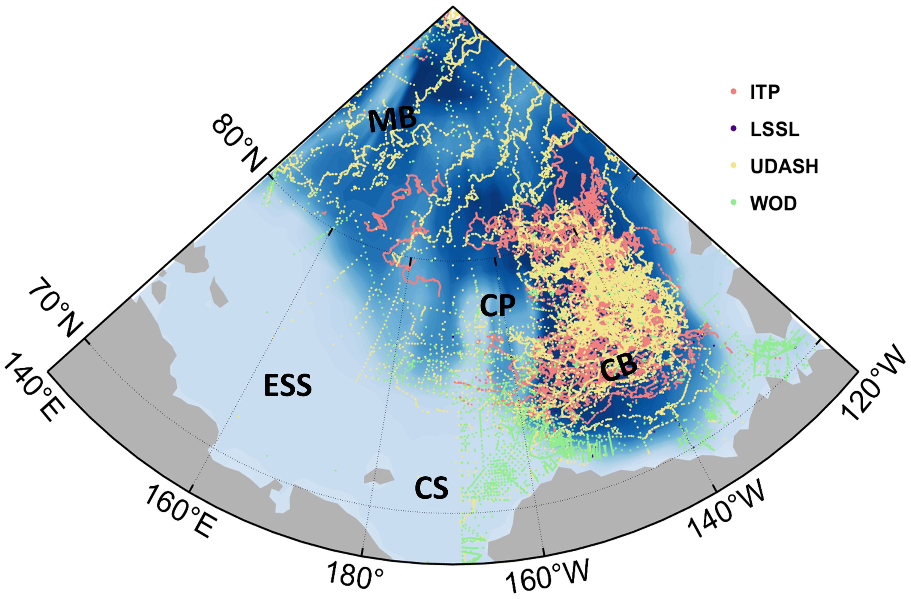
Figure 1. Topography of the Western Arctic Ocean. The map also includes the Canada Basin (CB), Chukchi sea (CS), the Chukchi Plateau (CP), East Siberian Sea (ESS) and Makarov Basin (MB).

The presence of sea ice severely limits the availability of salinity data in the Arctic Ocean, posing significant challenges to meeting the demands of current research. Behrentdt et al. (2018) collected a large amount of observed data to form a Unified Database for Arctic and Subarctic Hydrography for the period 1980-2015, however, there is a notable absence of hydrological data for recent years. In recent years, highly developed measurement techniques were especially designed for operation in the Arctic environment. Moreover, there is an increasing number of research initiatives and international collaborations, exemplified by the Beaufort Gyre Exploration Project (BGEP), which has produced a substantial volume of hydrographic data in the Western Arctic Ocean and subarctic seas (Rabe et al., 2014). Despite the heightened focus on polar observation initiatives, the temporal and spatial continuity of observational data continues to pose a significant challenge to our exploration of the Arctic. Shipborne observations of CTD and ITP (Ice-Tethered Profiler) data are sporadic, posing challenges in obtaining reliable salinity observations. The accuracy of both model and reanalysis data is frequently subpar. Our research specifically focuses on a case study of investigating salinity product improved by multi-machine learning results evaluating and integrating within Western Arctic Oceans.

The advancement of stochastic computer science and technology in recent years has led to an increasing utilization of machine learning methods across various domains. Machine learning methods have already demonstrated their efficacy in data generation tasks. The machine learning model refers to the algorithm that learns from input features. This can be conceptualized as a system that generates predictions based on input features. Readily accessible atmospheric and sea ice data are utilized as input features for salinity prediction, which is subsequently extrapolated using a validated model. Various machine learning models exhibit significant inter-model differences in salinity prediction; consequently, we have employed six machine algorithms to reconstruct salinity product. While traditional statistical regression methods demonstrate some efficacy in data reconstruction, their accuracy and applicability are constrained by the complex nonlinear relationships inherent in the atmosphere-ice-ocean system. In contrast, machine learning excels at addressing complex nonlinear interactions and is well-suited for data generation. Recently, it has seen extensive application and advancement in this domain (Wang et al., 2022; Chen et al., 2024). Previous studies have primarily concentrated on middle and low latitudes where data availability is substantial, while salinity is crucial for understanding the halocline dynamics of the Arctic Ocean; however, there is a paucity of research utilizing machine learning reconstruction methods to generate reliable salinity data for the high-latitude Arctic Ocean. Consequently, this paper employs several machine learning methods to produce dependable salinity data surpassing widely used dataset like ORAS5 in the Western Arctic Ocean.

This study performed machine learning training on sea level pressure, sea ice concentration, sea ice drift, as well as a large amount of quality-controlled CTD (WOD18, UDASH and ITP) data and EN4. The datasets were merged to generate a salinity product with a resolution of 0.5°×0.25° above 1000m for the period spanning from 2003 to 2022, encompassing a total of 48 vertical layers. The performance of machine learning was assessed not only through RMSE, but also by evaluating the uncertainty resulting from data merging and post calibrating processes. The salinity of ORAS5 datasets were employed to investigate the Beaufort Gyre and Arctic Ocean Hall et al., 2021. The accuracy and reliability of salinity product was validated through comparisons with ORAS5, as well as observed freshwater content and halocline depth in the Beaufort Gyre region.

2 Data and methodology

Our goal is to generate a set of salinity products that can be used to analyze variations in freshwater and halocline depth in the Western Arctic Ocean in recent years. The procedure of generating the salinity product is primarily divided into four key modules: data selection, machine learning, data merging, and post calibration (Figure 2).

Figure 2

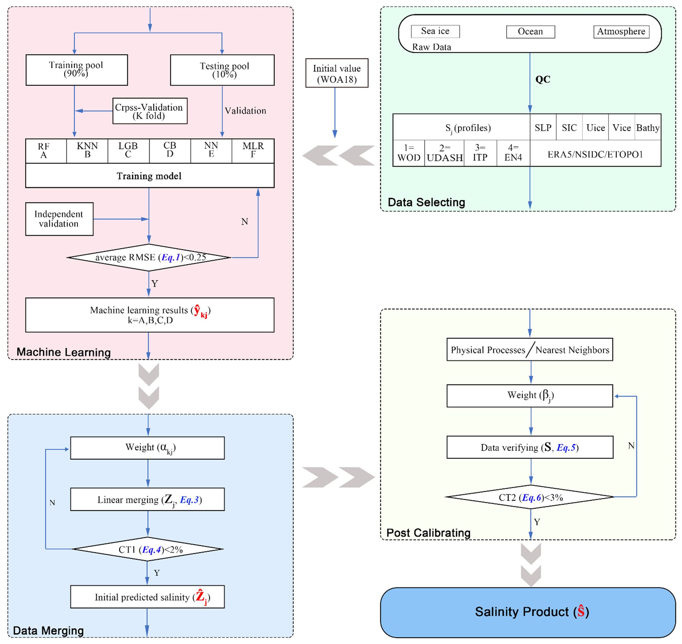
Figure 2. Procedure for generating the salinity product in the Western Arctic Ocean through a data mining-based machine learning method.

2.1 Data selecting

2.1.1 Data

We have collected a large amount of CTD salinity data. The CTD data was utilized in this study, which includes the WOD18, UDASH and ITP. The spatial distribution of CTD data from these different sources exhibits some degree of overlap, yet notable disparities persist. The World Ocean Database (WOD) is the world’s largest collection of uniformly formatted, quality controlled, publicly available ocean profile data (https://www.ncei.noaa.gov/access/world-ocean-database/bin/getwodyearlydata.pl?Go=TimeSorted, last access: 8 December 2023). Unified Database for Arctic and Subarctic Hydrography (UDASH) is a unified and high-quality temperature and salinity data set for the Arctic Ocean and the subpolar seas north of 65°N for the period 1980-2015 (https://essd.copernicus.org/articles/10/1119/2018/, last access: 8 December 2023). Sea ice presents a significant impediment to sustained observation of the Arctic Ocean. Researchers designed and field tested an automated, easily-deployed ITP for Arctic study. Building on the ongoing success of ice drifters that support multiple discrete subsurface sensors on tethers and the WHOI-developed Moored Profiler instrument capable of moving along a tether to sample at better than 1-m vertical resolution (https://www2.whoi.edu/site/itp/data/, last access: 8 December 2023).

This study interpolates all data onto the vertical depth grid of the WOD. Most of the CTD data was collected in late summer and early autumn (August to October), while the least CTD data was collected in June. The observed data is mainly concentrated in the Canada Basin, with very few observed data in the East Siberian Sea (Figure 3). After 2003, ITP provided a substantial amount of in situ CTD data, enabling the generation of gridded data for the period from 2003 to 2022. Considering the temporal and spatial discontinuity of the observed data, we have introduced EN4 reanalysis data (https://www.metoffice.gov.uk/hadobs/en4/, last access: 8 December 2023). Furthermore, considering the influence of the atmosphere and sea ice on the ocean, we have also incorporated SLP (Sea Level Pressure) data from ERA5 (https://cds.climate.copernicus.eu/cdsapp#!/dataset/reanalysis-era5-single-levels-monthly-means?tab=form, last access: 8 December 2023) and sea ice concentration and sea ice drift data from National Snow and Ice Data Center (NSIDC) (https://nsidc.org/home, last access: 8 December 2023). We use monthly salinity provided by the European Centre for Medium-Range Weather Forecasts (ECMWF) through the Ocean Reanalysis System’s version 5 (ORAS5), which uses the Nucleus for European Modeling of the Ocean (NEMOv3.4) for its ocean model coupled with a sea ice model to assess the performance of salinity product. In the data selecting, this study synthesizes previous literature and selected the sea level pressure, sea ice concentration, and sea ice drift data of the Western Arctic Ocean as training variables for machine learning.

Figure 3

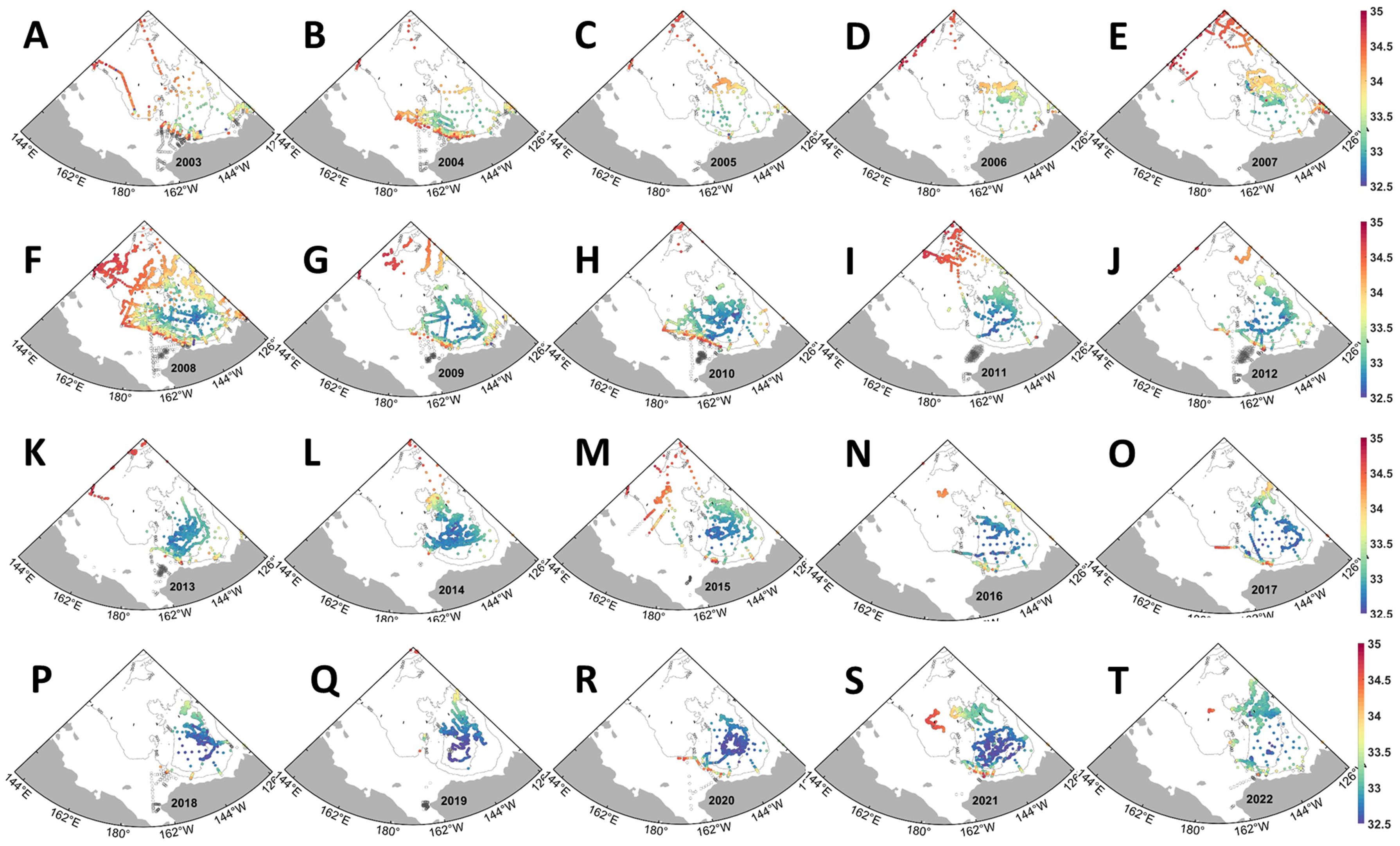
Figure 3. (A–T) Annual sea surface salinity from 2003 to 2022 in the Western Arctic Ocean. The colored dots represent the sea surface salinity at the CTD stations.

The CTD data collected includes a variety of issues such as missing values, outliers, and duplicates as well as gaps in dates and missing or incorrect latitude and longitude information. Therefore, the collected raw data underwent pre-processing. Under normal circumstances, missing data were interpolated, entries that could not be completed were removed, and duplicate data were eliminated. The pre-processing of our raw data primarily entails two quality control (QC) steps. Firstly, WOD18 offers quality-controlled data, with each data accompanied by extensive metadata, and every data value is associated with a corresponding quality control flag. We selected the highest quality data, specifically those associated with flags 0 and 1. Secondly, we removed invalid profile profiles from the datasets.

2.1.2 Initial value and independent validation data

World Ocean Atlas 18 (WOA18) (Zweng et al., 2019) salinity consists of a description of data analysis procedures and horizontal maps of climatological distribution fields of salinity at selected standard depth levels of the World Ocean on a one-degree and quarter-degree latitude-longitude grids. The series are used so frequently that they have become known generically as the “Levitus Climatology”. The observational-based gridded product WOA18 was utilized to evaluate the performance of the Arctic Subpolar Gyre State Estimate (ASTE) in the Arctic Ocean (Zhong et al., 2024). We propose that the salinity of the Arctic Ocean can be categorized into two components: the initial value determined by WOA18, which reflects the constrained climate state, and the subsequent changes in salinity predicted through our machine learning methods based on this climate state. WOA18 data is also used to evaluate the performance of generated salinity product.

Shipboard hydrographic data and water sampling observed on board the CCGS (Canadian Coast Guard Shipboard) LSSL (Louis S. St-Laurent) are carried out at about 30 standard sites on each cruise (https://www2.whoi.edu/site/beaufortgyre/data/ctd-and-geochemistry/, last access: 8 December 2023), the CTD data of LSSL collected during the 2004 expedition was not utilized. The potential temperature and density of the CTD data in 2004 are evidently anomalous, suggesting a potential issue with the data storage process, thus rendering them unsuitable for this study.

2.2 Machine learning

In the machine learning training process, we selected six widely used methods: Random Forest (RF), K Nearest Neighbor (KNN), LightGBM (LGB), CatBoost (CB), Neural Network (NN), and Multilinear Regression (MLR). We determined the optimal values of different machine learning method using optuna hyperparameter methods (code from https://github.com/optuna/, last access: 20 March 2024) and GridSearchCV (from scikit-learning). We employed six distinct machine learning methods to train the CTD (WOD18, UDASH, ITP) and EN4.

The issue of overfitting must be addressed during the machine learning process. The datasets utilized for prediction from each year were randomized; subsequently, 90% of the data was designated for training purposes, forming the training pool, while the remaining 10% was reserved for testing purposes, constituting the testing pool. Training pool (90%) and testing pool (10%) in this study are divided by space.

It is necessary to evaluate the accuracy of any model based on certain error metrics before applying it to specific scenarios. Common model evaluation metrics include mean absolute error (MAE), root-mean-square error (RMSE). The mean squared error (MSE) is the standard deviation of the residuals (prediction error), and the residuals are the distances between the fitted line and the data points (i.e., the residuals show the degree of concentration of the reconstructed data around the regression line). In regression analysis, RMSE is frequently used to verify experimental results. To assess bias, the RMSE needs to combine the magnitude of the model data and is calculated as follows:

$\begin{array}{ll}RMS{E}_{kj}=\sqrt{\frac{1}{n}{\displaystyle \sum _{i=1}^n{(y_{ikj}-{\widehat{y}}_{ikj})}^2} }& \text{1}\end{array}$

where n is the number of data points; k represents different machine learning methods, and there are six types in total, which are RF, KNN, LGB, CB, NN, MLR; j=1 represents WOD18 data, j=2 represents UDASH data, j=3 represents ITP data and j=4 represents EN4 data; y is the training target; $\widehat{y}$ is the prediction result after machine learning training.

Taking the results from 2008 of Random Forest as an example (Figure 4), our analysis revealed that salinity predictions at 200 m are more accurate than those at the surface (15 m) based on the verification results from the testing pool, and it was observed that the RMSE for EN4 is smaller than that for CTD. However, what is exciting is that even for the weakest prediction ability of CTD at the surface, the RMSE is less than 0.35 psu. Therefore, our evaluation of the machine learning results will mainly focus on the surface with larger prediction errors by RMSE.

Figure 4

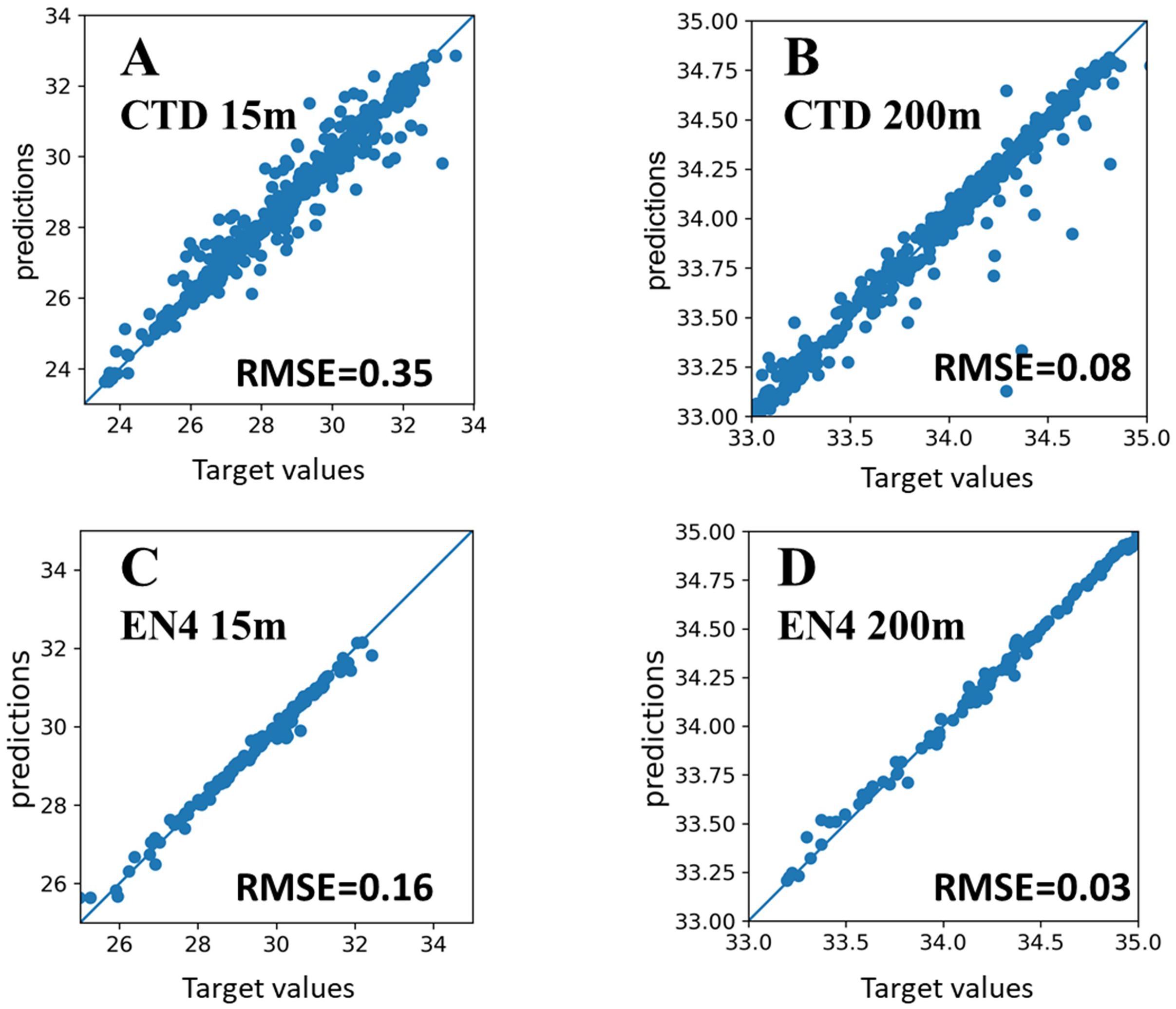
Figure 4. Comparisons between the predicted salinity and train target salinity values in the testing pool for the Random Forest in 2008. (A) CTD salinity at 15m, (B) CTD salinity at 200m, (C) EN4 salinity at 15m, (D) EN4 salinity at 200m.

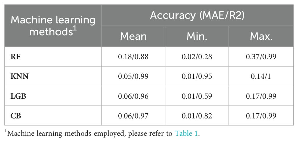
In addition to Random Forest (RF), we also evaluated the predictive performance of surface salinity using five other machine learning methods (Table 1), with assessment based on RMSE as outlined below:

Table 1

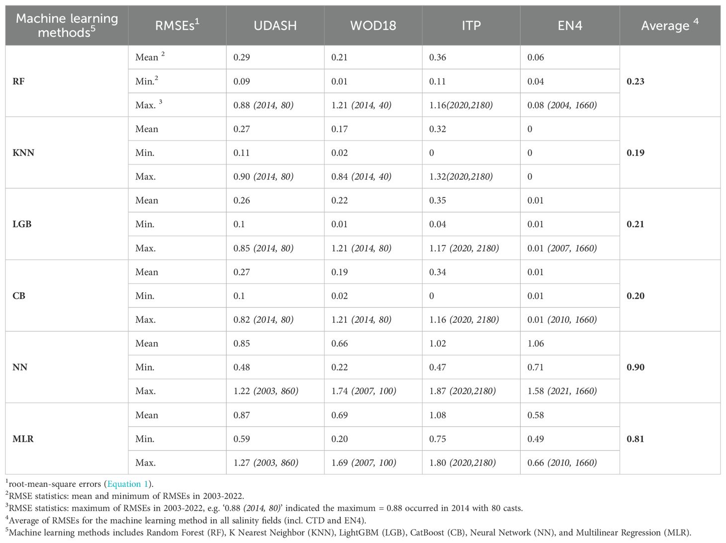
Table 1. Evaluation of predicted surface salinity of different CTD sources in the testing pool using different machine learning methods.

We selected four machine learning methods whose predictions is closer to the training target of sea surface salinity (with the average of RMSE less than 0.25), which are RF, KNN, LGB, and CB (Table 1). We employed the K-fold cross-validation during the machine learning training process in the training pool. We used R² to verify the ability of machine learning training which is calculated as follows:

$\begin{array}{ll}{R}^2=1-\frac{{\sum }_{i=1}^n{(y_i-\widehat{y})}^2}{{\sum }_{i=1}^n{(y_i-\overline{y_i})}^2}& \text{2}\end{array}$

where n is the number of data points; y is the training target data; $\widehat{y}$ is the prediction result after machine learning training. We also selected RF, KNN, LGB, and CB based on the results of cross-validation. The four selected machine learning methods demonstrate superior prediction results for EN4 in comparison to CTD. The errors arising during the prediction process mainly come from the prediction of CTD salinity. The annual variations in the predictive capabilities of these four machine learning methods are highly significant. The prediction results for RF were the best in 2005 and 2016, and the worst in 2020, KNN had the best prediction results for 2016 and 2017, and the worst prediction results for 2020. LGB had the best forecast results for 2016 and 2017, and the worst forecast results for 2003. CB had the best forecast results for 2016 and 2017, and the worst forecast results for 2003. In the same year, some machine learning predictions are good while others are poor. For example, in 2020, the mean RMSE of RF (0.32) and KNN [CTD (0.45)] were poor, but the predictions of LGB (0.14) and CB (0.14) were good.

RMSE is the spatial average result (Table 1), so only considering the numerical value of RMSE may ignore the predictive ability of machine learning methods on different regions in space. After training, we selected four machine learning methods with the mean RMSE less than 0.25, which are RF, KNN, LGB, and CB. We take the example of the prediction error of surface salinity in 2008 (predicted value minus training target value) to analyze the salinity prediction ability of machine learning methods in different regions. Machine learning models exhibit significant spatial differences in predicting the salinity of CTD (Figure 5). Specifically, there are larger prediction errors in the Chukchi Sea, Chukchi Sea Shelf, southern continental shelf slope of the Beaufort Gyre and central Canada basin. The largest error occurred in the Chukchi Sea, which may be due to the influence of Pacific water on the salinity of the upper layer of the Western Arctic Ocean. The four machine learning methods for predicting surface salinity in EN4 are all very good. KNN, LGB, and CB even have negligible prediction errors. RF exhibits a significant spatial distribution in predicting surface salinity in EN4, characterized by overestimations in the southeastern Canada Basin and the Western East Siberian Sea, with prediction errors remaining below 0.2 psu. The predictions are underestimated in the Chukchi Sea and the East Siberian Sea. The prediction errors of different machine learning methods vary, so different weights need to be considered in the data mergence process.

Figure 5

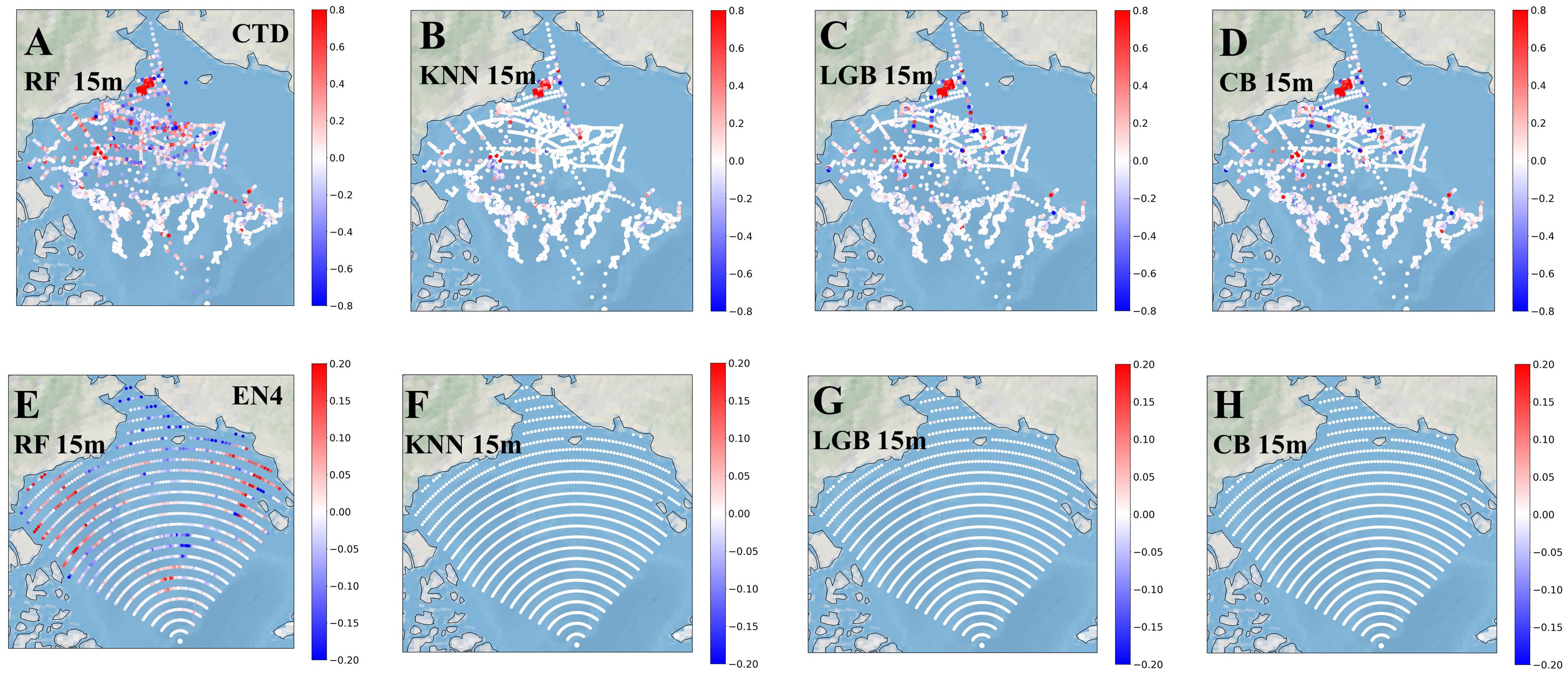
Figure 5. Error between the predicted salinity and real salinity values for the training pool and testing pool in 2008. (A–D) Evaluation of CTD salinity at 15m reconstructed by RF, KNN, LGB and CB. (E-H) Evaluation of EN4 salinity at 15m reconstructed by RF, KNN, LGB and CB.

In machine learning process, the dataset is typically partitioned into three distinct subsets: the training set, the validation set, and the testing set. The testing pool serves to evaluate the performance of the final selected optimal model. To ensure the accuracy and reliability of predicted salinity generated by machine learning models and avoid overfitting, we employed the independent LSSL CTD data as an independent dataset for independent validation (Table 2). The selected four machine learning methods can be used to generated salinity product in Western Arctic Ocean.

Table 2

Table 2. Independent validation of selected machine learning model.

2.3 Data merging and post calibrating

During the data merging process, the training results of the four most effective machine learning models were combined to generate initial predicted salinity. MAE represents the average absolute difference between the in situ data (true values) and the training model results (predicted values). The sign of these differences is ignored so that cancelations between positive and negative values do not occur. RMSE and MAE are primarily used to represent the uncertainty in reconstructed datasets. In this study, we choose MAE as the criterion for assessing uncertainty. We introduced weights and defined uncertainty, for selecting weights ${\alpha }_{kj}$. The initial merged results ($Z_j$):

$\begin{array}{ll}{Z}_j={\displaystyle {\sum }_{k=1}^4{\alpha }_{kj}{\widehat{y}}_{kj}}& \text{3}\end{array}$

Where k represents different machine learning methods, and there are four types in total, which are RF, KNN, LGB, CB; j=1 represents WOD18, j=2 represents UDASH, j=3 represents ITP and j=4 represents EN4 data, ${\widehat{y}}_{kj}$ is different training results of machine learning methods based on CTD (WOD18, UDASH, ITP) and EN4.

The uncertainty of data merging ($\text{CT}1$) represent the average of MAE between the initial merged results ($Z_j)$ based on CTD (WOD18, UDASH, ITP) and EN4 and the extracted reconstruction results obtained from the four machine learning methods, which is calculated as follows:

$\begin{array}{ll}\text{CT}1=\frac{1}{4}{\displaystyle {\sum }_{k=1}^4}\frac{\left|{\widehat{y}}_{kj}-Z_j\right|}{Z_j}\times 100\%& \text{4}\end{array}$

We determined the threshold for CT1 based on a 2% of mean surface salinity from 2003 to 2022, corresponding to 0.5 psu. The data merging process described in this study concludes when CT1 falls below the threshold, resulting in the acquisition of the initial predicted salinity (${\widehat{Z}}_j$).

During the post calibrating process, initial predicted salinity was utilized to generate salinity product. when there are at least three CTD measurements available in the vicinity of the grid point, the salinity value of the point is formed by merging the EN4 initial predicted salinity and the CTD (WOD18, UDASH, ITP) initial predicted salinity according to weights (${\beta }_{\dot{j}}$); otherwise, the salinity value of the point is taken as the EN4 prediction result. We need to check that salinity results (S)

$\begin{array}{ll}S={\displaystyle {\sum }_{j=1}^4{\beta }_{\dot{j}}{\widehat{Z}}_j}& \text{5}\end{array}$

The uncertainty of post calibrating (CT2) represent the average of MAE between the initial salinity results (S) obtained from CTD (WOD18, UDASH, ITP) and EN4, which is calculated as follows:

$\begin{array}{ll}\text{CT}2=\frac{1}{4}{\displaystyle {\sum }_{j=1}^4}\frac{\left|{\widehat{Z}}_j-S\right|}{S}\times 100\%& \text{6}\end{array}$

We determined the threshold for CT2 based on a 3% of mean surface salinity from 2003 to 2022, corresponding to 0.8 psu. When CT2 falls below the prescribed threshold, the post-calibration procedure is adjudged accomplished, thereby generating salinity product ($\widehat{S}$).

3 Result and discussion

The uncertainty of the salinity product in this study (represented by MAE) includes three parts: one part is the uncertainty generated during the machine learning training process, with an uncertainty of 0.1 psu for surface salinity predictions derived from CTD salinity and 0.01 psu for those based on EN4 salinity; the other parts include uncertainties in data merging (Figures 6A, B) and post calibrating (Figure 6C). Two sets of initial predicted salinity are utilized for data merging in the machine learning methods: EN4 and CTD (WOD18, UDASH, ITP). The uncertainty generated shows that the uncertainty constrained by CTD data is larger in the central Canada Basin and the Chukchi Sea Shelf and its adjacent ocean, reaching 0.46 psu in the central Canada Basin. The uncertainty constrained by EN4 data is larger in the central Canada Basin and the East Siberian Sea, reaching 0.12 psu in the East Siberian Sea. The uncertainty generated during the post calibrating process is highest in the Canada basin, with a maximum value of 0.7 psu.

Figure 6

Figure 6. Spatial pattern of sea surface salinity uncertainty (psu) during the data merging (A), CTD; (B), EN4) and post calibrating (C).

We used salinity product to calculate the freshwater content in the Beaufort Gyre region (black box in Figure 7A). To validate the performance of the salinity product in calculating freshwater content (Figure 7), we also utilized the freshwater content data provided by BGEP, which is derived from LSSL data, for comparison. On the other hand, the research of Hall et al., 2021 showed that the salinity of ORAS5 can be used to calculate the freshwater content of the Arctic Ocean, and we also introduced the results of the freshwater content calculation of ORAS5 (Figure 7B). The FWC (freshwater content) was computed relative to 34.8 psu following Proshutinsky et al. (2009):

Figure 7

Figure 7. Temporal and spatial variation of Freshwater Content (m). (A) Shadow represents Mean FWC from 2003 to 2022 derived from salinity product, color dots represent FWC provided by BGEP. (B) Time series of FWC and LSSL CTD casts in Beaufort Gyre region, Beaufort Gyre region is the black box in (A).

$\begin{array}{ll}\text{FWC}={\int }_{z34.8}^{zsurface}\left(\frac{34.8-\text{s}(\text{z})}{34.8}\right)\text{dz}& \text{7}\end{array}$

The absolute errors between the freshwater content derived from BGEP and those from the generated salinity product as well as ORAS5 are 0.98 m, 4.28 m, respectively. Using the salinity product to calculate the freshwater content in the Beaufort Gyre region can improve the accuracy compared to ORAS5. We compared the spatial distribution of freshwater content calculated from salinity product with that provided by BGEP. Certain regions on the Mendeleev Ridge exhibit substantial freshwater content, potentially resulting from freshwater advection originating from either the East Siberian Sea or the Beaufort Gyre.

The depth of halocline base plays an important role in studying the Beaufort Gyre dynamics (Manucharyan et al., 2016). The depth of the halocline base is determined by taking the 33.9 psu contours (Lin et al., 2023; Nyugen et al., 2012). All salinity data used were interpolated vertically to 2 m to calculate the depth of the halocline base. The salinity product, ORAS5 and WOA18 estimated the halocline depth in Beaufort Gyre region of 192.35 m, 177.00 m and 191.04 m, respectively (Figure 8D). The salinity product enables a more accurate calculation of the depth of the halocline. Compared with the results of ORAS5, the depth of halocline calculated by salinity product increased significantly in the 2000s. We compared the spatial distribution characteristics of the bottom halocline and WOA18 obtained from salinity product (Figures 8A–C). The depth of halocline is the deepest in the Canada Basin, but the salinity product results are shallower and further east than WOA18. The depth of the halocline base calculated by salinity product is obviously 21m shallower in the southwest of the Canada Basin and 23m deeper in the north of the East Siberian Sea.

Figure 8

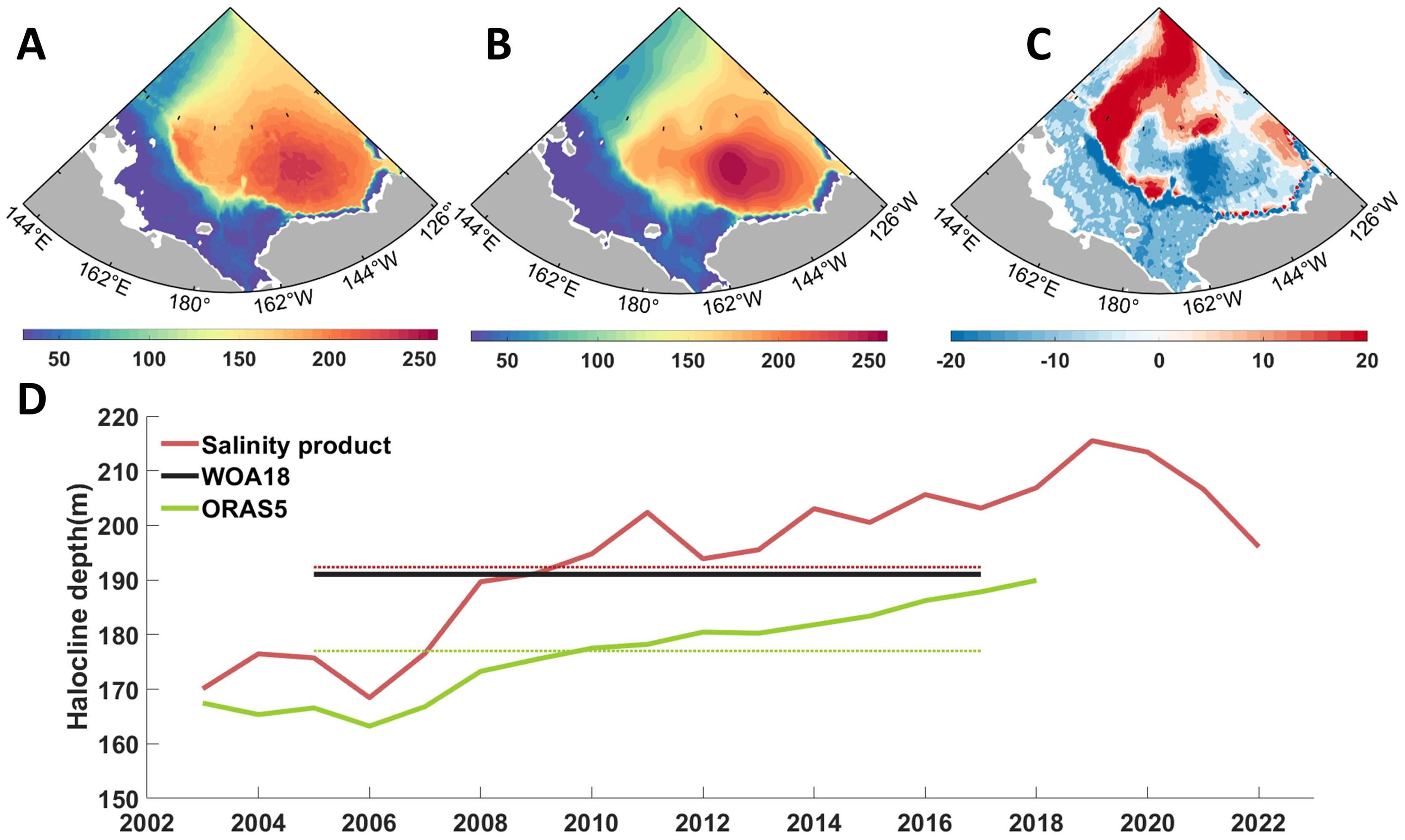
Figure 8. Temporal and special variation of halocline depth (m). (A) Mean halocline depth from 2005 to 2017 derived from salinity product (B) Mean halocline base depth from 2005 to 2017 derived from salinity of WOA18. (C) Mean halocline depth difference between salinity product and WOA18 from 2005 to 2017. (D) Time series of halocline depth in Beaufort Gyre region. The dashed line is the mean halocline depth of ORAS5 and salinity product.

The results of salinity product indicate that the study enhances Arctic Ocean salinity data using machine learning and also provides a precise understanding of freshwater content and depth variations in the Beaufort Gyre, surpassing widely used dataset like ORAS5. Salinity product can be utilized to examine the accumulation and release of freshwater within the Beaufort Gyre, serving as a reliable supplement to salinity data in the investigation of Beaufort Gyre halocline dynamics associated. The surface salinity is characterized by low salinity in the central Canada Basin and the East Siberian Sea, which indicates the accumulation of freshwater there (Figure 9). The continuous decrease in surface salinity before 2011 and the continuous increase in surface salinity after 2011 indicate that freshwater accumulated mainly at the surface before 2011 and decreased after 2011, which support the recent major freshening event from 2012 to 2016 in the North Atlantic (Holliday et al., 2020). In the east-west direction, the characteristics of low surface salinity expanded westward from 2003 to 2013 and eastward from 2014 to 2022, thereby supporting the conclusion that the Beaufort Gyre has expanded westward (Regan et al., 2019; Armitage et al., 2017) and shrunk eastward (Lin et al., 2023). In the north-south direction, the characteristics of low surface salinity expanded northward in 2007, 2008, 2015, and 2016. The surface salinity of the East Siberian Sea experienced a significant decrease in 2008 and has since remained at reduced levels. According to the characteristics of surface ocean circulation (Armitage et al., 2017), surface freshwater in the East Siberian Sea may enter the Beaufort Gyre or flow out of the Arctic Ocean along the transpolar drift. The characteristics of sea surface salinity indicate that Pacific water flows partially into the northern Chukchi Sea, the Canada Basin, and the CAA (Canadian Arctic Archipelago) along the Alaskan coastal current. The decreased sea surface salinity of the Alaskan coastal current suggests a diminished transport of Pacific water along this route, indicating a weakening of the Alaskan coastal current, potentially influenced by the intensified Beaufort Gyre.

Figure 9

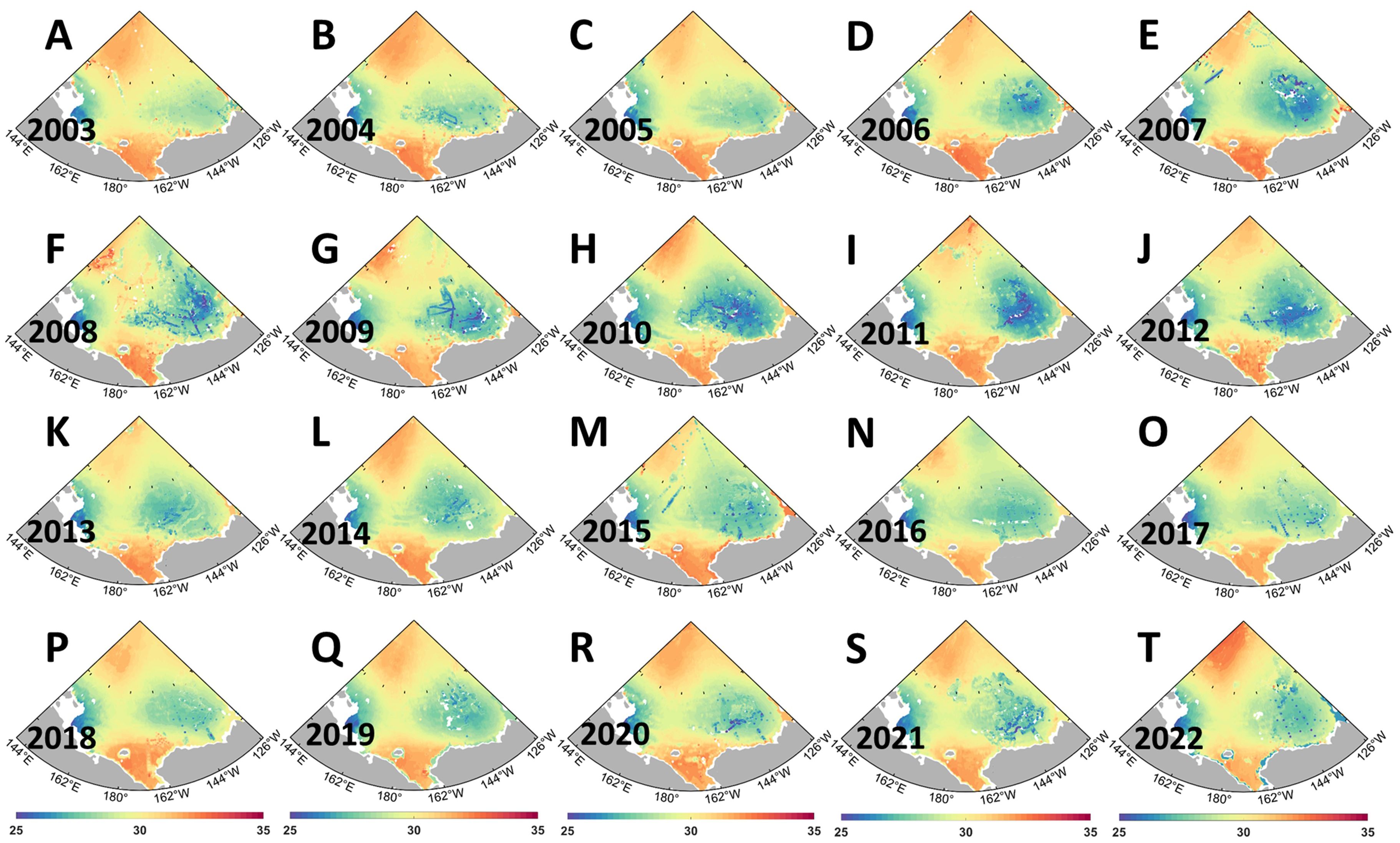
Figure 9. (A–T) Annual sea surface salinity fields in the Western Arctic ocean from 2003 to 2022. The color dots represent the measured CTD salinity, and the white dots represent the measured sites that were deleted after quality control. Shadow represents the sea surface salinity of salinity product.

To examine the salinity distribution at the base of the halocline, approximately 200 meters below the surface in the Western Arctic Ocean, we analyzed the salinity distribution at this depth. The results of salinity product indicate that salinity at 200 m is characterized by low salinity in the central Canada Basin which indicates the accumulation of freshwater in Canada Basin. Unlike the sea surface salinity, the salinity at 200 m has remained a slow downward trend after a rapid decline before 2008. This indicates that freshwater in the Canada Basin remained relatively stable following a rapid accumulation prior to 2008. Prior to 2008, freshwater in the Western Arctic Ocean accumulated in substantial quantities at both the surface and the base of the halocline. Following 2008, surface water experienced a significant decrease while salinity at the bottom of the halocline continued to rise, suggesting that freshwater may be redistributed within the Arctic Ocean through westward and northward expansion into the Makalov Basin (Bertosio et al., 2022), transported out of the Arctic Ocean (Zhang et al., 2021), or pooled deeper within the water column. From 2003 to 2013, the range of low salinity characteristics of the halocline depth expanded, indicating that the area of freshwater reservoir expanded and the area of Beaufort Gyre expanded. The salinity at 200m in 2022 increases significantly, indicating that there may be a freshwater migration process in 2022.

We conducted an analysis to determine the significance of five input variables in predicting salinity, which serves as a reliable indicator for identifying the key factors influencing salinity changes (Figure 10). However, it is essential to recognize the potential interactions among various variables. The significance of different factors varies when predicting salinity in both EN4 and CTD datasets. Notably, both datasets consistently identify sea level pressure as the primary influencing factor for surface salinity prediction, while sea ice concentration emerges as the principal determinant when forecasting salinity at a depth of approximately 200 m. The impact of sea ice movement on the surface is more significant than that on the bottom of the halocline. The meridional ice speed is advantageous for salinity prediction using CTD data, while the zonal flow speed is advantageous for salinity prediction using EN4 data. However, the contribution of water depth factors varies. CTD data indicates that water depth has a dominant influence on salinity prediction in deep layers, whereas EN4 data shows the opposite trend. Salinity is closely associated with freshwater distribution. The transport and accumulation of surface freshwater are regulated by the sea level pressure field, and the melting of sea ice exerts a greater impact on salinity compared to its movement.

Figure 10

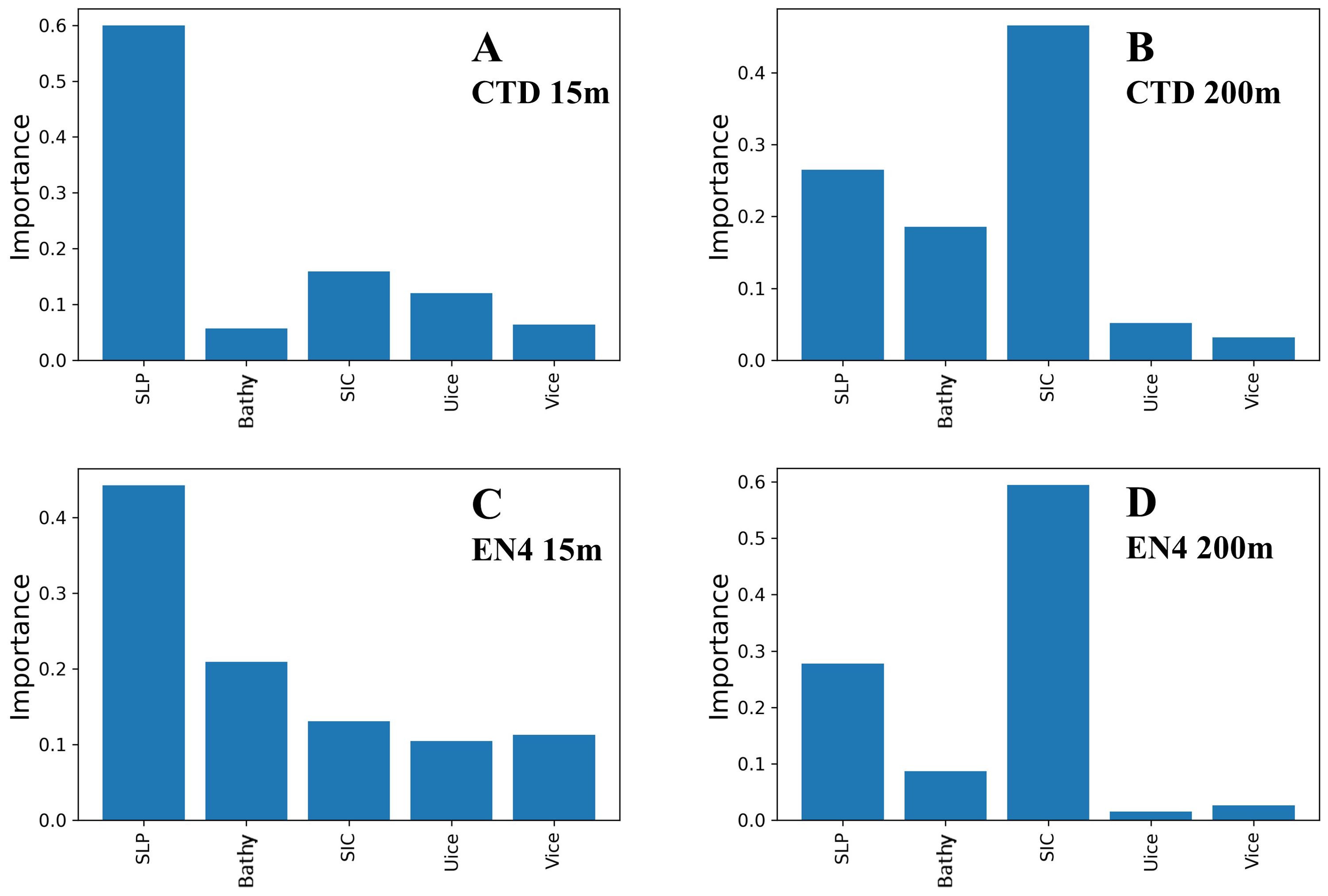
Figure 10. The importance of different input variables at sea surface and halocline depth in predicting CTD (WOD18, UDASH, ITP) salinity and EN4 salinity. (A) CTD salinity at 15m, (B) CTD salinity at 200m, (C) EN4 salinity at 15m, (D) EN4 salinity at 200m.

4 Summary

Based on data mining-based machine learning method, we provided an annual salinity product for the Western Arctic Ocean with a resolution of 0.5°×0.25°for the period spanning from 2003 to 2022. This was achieved by establishing correlations between bathymetry, sea ice dynamics, atmospheric conditions, and seawater salinity. The input variables employed in our machine learning model encompass sea level pressure from ERA5 and sea ice concentration and motion from NSIDC, as well as ETOPO1 dataset. After filtering, we employ four machine learning methods (Random Forest, K Nearest Neighbor, LightGBM, CatBoost) to train salinity data obtained from CTD (WOD18, UDASH, ITP) and EN4. Utilizing multiple machine learning methods can mitigate the impact of inherent flaws in a specific method on the results. During data integration, varying weight combinations of variables greatly affect uncertainty; therefore, we implement an uncertainty threshold to constrain appropriate weights. There are some limitations in this study, including uncertainty from data merging and post calibration processes, potential inaccuracies in the reconstructed salinity product, and the limited focus on the Western Arctic Ocean, leaving the method’s applicability to other regions unexplored.

An accurate salinity product is crucial for understanding the dynamics of the Beaufort Gyre and the redistribution of freshwater in the Beaufort Gyre in the Western Arctic Ocean. Hall et al. 2021 demonstrated that ORAS5 salinity data are applicable for studies of the Arctic Ocean. However, when compared ORAS5, salinity-derived freshwater content aligns more closely with BGEP estimates, suggesting superior accuracy in FWC calculations. Furthermore, considering the precision of halocline depth, salinity products exhibit greater accuracy than ORAS5. The findings from salinity product reveal a significant increase in freshwater content throughout the upper 200 m of the Beaufort Gyre during the 2000s; however, surface freshwater decreased while subsurface freshwater continued to accumulate during the 2010s. It is likely that surface freshwater has been redistributed toward the Makalov Basin (Bertosio et al., 2022), potentially accumulating in subsurface layers due to Ekman Pumping.

The importance of various factors varies when predicting salinity in both EN4 and CTD (WOD18, UDASH, ITP) data. Interestingly, both datasets consistently highlight sea level pressure as the primary influential factor for surface salinity prediction, while sea ice concentration emerges as the main determinant when forecasting salinity at a depth of approximately 200 m (corresponding to the halocline depth) (Figure 10). The reconstruction of salinity data in the Western Arctic Ocean holds significant scientific value. However, further research is needed to incorporate other variables that influence salinity, such as the Pacific Ocean inflow the and the ventilation process in the Chukchi Sea, into the salinity data reconstruction process.

The salinity field of the Western Arctic Ocean is taken as an example to construct a novel data mining method for polar sea areas, utilizing multiple machine learning methods that integrate multiple data sources and incorporate physical processes. The application potential of this method extends beyond the salinity field and includes other related fields like hydrometeorology, sea ice thickness, polar biogeochemistry, among others. It effectively utilizes multi-machine learning results for data evaluation and integration.

Data availability statement

The datasets presented in this study can be found in online repositories. The names of the repository/repositories and accession number(s) can be found in the article/supplementary material.

Author contributions

ST: Conceptualization, Data curation, Formal analysis, Investigation, Visualization, Writing – original draft, Writing – review & editing. LD: Conceptualization, Funding acquisition, Resources, Supervision, Writing – review & editing. JL: Supervision, Writing – review & editing.

Funding

The author(s) declare that financial support was received for the research, authorship, and/or publication of this article. This work was supported by the National Natural Science Foundation of China (Grant No. 42230405, 41976217, and 41576020) and the Global Change Research Program of China (No. 2015CB953902).

Acknowledgments

We collected a large number of public data, collected during numerous expeditions and cruises over several decades. It is impossible to mention all researchers who have contributed to these projects. We therefore thank all these people for the gigantic effort, the huge amount of work and for making their data freely available.

Conflict of interest

The authors declare that the research was conducted in the absence of any commercial or financial relationships that could be construed as a potential conflict of interest.

Publisher’s note

All claims expressed in this article are solely those of the authors and do not necessarily represent those of their affiliated organizations, or those of the publisher, the editors and the reviewers. Any product that may be evaluated in this article, or claim that may be made by its manufacturer, is not guaranteed or endorsed by the publisher.

References

Armitage T. W., Bacon S., Ridout A. L., Petty A. A., Wolbach S., Tsamados M. (2017). Arctic Ocean surface geostrophic circulation 2003–2014. Cryosphere 11, 1767–1780. doi: 10.5194/tc-11-1767-2017

Crossref Full Text | Google Scholar

Behrendt A., Sumata H., Rabe B., Schauer U. (2018). UDASH – unified database for arctic and subarctic hydrography. Earth Syst. Sci. Data 10, 1119–1138. doi: 10.5194/essd-10-1119-2018

Crossref Full Text | Google Scholar

Bertosio C., Provost C., Athanase M., Sennéchael N., Garric G., Lellouche J. M., et al. (2022). Changes in freshwater distribution and pathways in the Arctic Ocean since 2007 in the Mercator Ocean global operational system. J. Geophysical Research: Oceans 127, e2021JC017701. doi: 10.1029/2021JC017701

Crossref Full Text | Google Scholar

Carmack E. C., McLaughlin F. A., Yamamoto-Kawai M., Itoh M., Shimada K., Krishfield R., et al. (2008). “Freshwater storage in the Northern Ocean and the special role of the Beaufort Gyre,” in Arctic–Subarctic Ocean Fluxes, Defining the Role of the Northern Seas in Climate, eds R. R. Dickson, J. Meincke, and P. Phines (Dordrecht: Springer), 145–169. doi: 10.1007/978-1-4020-6774-7_8

Crossref Full Text | Google Scholar

Carmack E. C., Yamamoto-Kawai M., Haine T. W., Bacon S., Bluhm B. A., Lique C., et al. (2016). Freshwater and its role in the Arctic Marine System: Sources, disposition, storage, export, and physical and biogeochemical consequences in the Arctic and global oceans. J. Geophysical Research: Biogeosciences 121, 675–717. doi: 10.1002/2015JG003140

Crossref Full Text | Google Scholar

Chen L., Wang Q., Zhu G., Lin X., Qiu D., Jiao Y., et al. (2024). Dataset of stable isotopes of precipitation in the Eurasian continent. Earth System Sci. Data 16, 1543–1557. doi: 10.5194/essd-16-1543-2024

Crossref Full Text | Google Scholar

Cornish S. B., Kostov Y., Johnson H. L., Lique C. (2020). Response of Arctic freshwater to the Arctic oscillation in coupled climate models. J. Climate 33, 2533–2555. doi: 10.1175/JCLI-D-19-0685.1

Crossref Full Text | Google Scholar

Giles K. A., Laxon S. W., Ridout A. L., Wingham D. J., Bacon S. (2012). Western Arctic Ocean freshwater storage increased by wind-driven spin-up of the Beaufort Gyre. Nat. Geosci. 5, 194–197. doi: 10.1038/ngeo1379

Crossref Full Text | Google Scholar

Hall S. B., Subrahmanyam B., Morison J. H. (2021). Intercomparison of salinity products in the Beaufort Gyre and Arctic Ocean. Remote Sens. 14, 71. doi: 10.3390/rs14010071

Crossref Full Text | Google Scholar

Holliday N. P., Bersch M., Berx B., Chafik L., Cunningham S., Florindo-López C., et al. (2020). Ocean circulation causes the largest freshening event for 120 years in eastern subpolar North Atlantic. Nat. Commun. 11, 585. doi: 10.1038/s41467-020-14474-y

PubMed Abstract | Crossref Full Text | Google Scholar

Lin P., Pickart R. S., Heorton H., Tsamados M., Itoh M., Kikuchi T. (2023). Recent state transition of the Arctic Ocean’s Beaufort Gyre. Nat. Geosci. 16, 485–491. doi: 10.1038/s41561-023-01184-5

Crossref Full Text | Google Scholar

Manucharyan G. E., Spall M. A., Thompson A. F. (2016). A theory of the wind-driven beaufort gyre variability. J. Phys. Oceanography 46, 3263–3278. doi: 10.1175/jpo-d-16-0091.1

Crossref Full Text | Google Scholar

Meneghello G., Marshall J., Campin J. M., Doddridge E., Timmermans M. L. (2018). The ice-ocean governor: Ice-ocean stress feedback limits Beaufort Gyre spin-up. Geophysical Res Lett, 45(20), 11-293. doi: 10.1029/2018GL080171

Crossref Full Text | Google Scholar

Muilwijk M., Hattermann T., Martin T., Granskog M. A. (2024). Future sea ice weakening amplifies wind-driven trends in surface stress and Arctic Ocean spin-up. Nat. Commun. 15, 6889. doi: 10.1038/s41467-024-50874-0

PubMed Abstract | Crossref Full Text | Google Scholar

Nguyen A. T., Kwok R., Menemenlis D. (2012). Source and pathway of the western arctic upper halocline in a data-constrained coupled ocean and sea ice model. J. Phys. Oceanography 42, 802–823. doi: 10.1175/jpo-d-11-040.1

Crossref Full Text | Google Scholar

Proshutinsky A., Krishfield R., Timmermans M. L., Toole J., Carmack E., McLaughlin F., et al. (2009). Beaufort Gyre freshwater reservoir: State and variability from observations. J. Geophys. Res. 114, C00A10. doi: 10.1029/2008JC005104

Crossref Full Text | Google Scholar

Proshutinsky A., Krishfield R., Toole J. M., Timmermans M. L., Williams W., Zimmermann S., et al. (2019). Analysis of the Beaufort Gyre freshwater content in 2003–2018. J. Geophysical Research: Oceans 124, 9658–9689. doi: 10.1029/2019JC015281

PubMed Abstract | Crossref Full Text | Google Scholar

Rabe B., Karcher M., Kauker F., Schauer U., Toole J. M., Krishfield R. A., et al. (2014). Arctic Ocean basin liquid freshwater storage trend 1992–2012. Geophysical Res. Lett. 41, 961–968. doi: 10.1002/2013gl058121

Crossref Full Text | Google Scholar

Regan H. C., Lique C., Armitage T. W. (2019). The Beaufort Gyre extent, shape, and location between 2003 and 2014 from satellite observations. J. Geophysical Research: Oceans 124, 844–862. doi: 10.1029/2018jc014379

Crossref Full Text | Google Scholar

Wang Z., Wang G., Guo X., Bai Y., Xu Y., Dai M. (2022). Spatial reconstruction of long-term (2003-2020) sea surface pCO2 in the South China Sea using a machine learning based regression method aided by empirical orthogonal function analysis. Earth System Sci. Data 2023, 1–30. doi: 10.5194/essd-15-1711-2023

Crossref Full Text | Google Scholar

Zhang J., Weijer W., Steele M., Cheng W., Verma T., Veneziani M. (2021). Labrador Sea freshening linked to Beaufort Gyre freshwater release. Nat. Commun. 12, 1229. doi: 10.2172/1766967

PubMed Abstract | Crossref Full Text | Google Scholar

Zhong W., Lan Y., Mu L., Nguyen A. T. (2024). The mixed layer salinity balance in the western Arctic Ocean. J. Geophysical Research: Oceans 129, e2023JC020591. doi: 10.1029/2023JC020591

Crossref Full Text | Google Scholar

Zweng M. M., Seidov D., Boyer T. P., Locarnini M., Garcia H. E., Mishonov A. V., et al. (2019). World Ocean Atlas 2018, Volume 2: Salinity. Mishonov Technical. NOAA Atlas NESDIS 82, 50pp.

Google Scholar