- 1College of Computer Science and Technology, National University of Defense Technology, Changsha, China
- 2College of Meteorology and Oceanography, National University of Defense Technology, Changsha, China
- 3School of Computer Science and Engineering, Central South University, Changsha, China
Accurately predicting the spatio-temporal evolution trends and long-term dynamics of three-dimensional ocean temperature and salinity plays a crucial role in monitoring climate system changes and conducting fundamental oceanographic research. Numerical models are the most prevalent of the traditional approaches, which are often too complex and lack of generality. Recently, with the rise of AI, many data-driven methods are proposed. However, most of them take no consideration of natural physical laws that may cause issues of physical inconsistency among different variables. In this paper, we proposed PGTransNet, a novel physics-guided transformer network for 3D Ocean temperature and salinity forecasting. This model is based on Vision Transformer, and to enhance the performance we have three aspects of improvements. Firstly, we design a loss function that deliveries the physical relationship among temperature, salinity and density by fusing the Thermodynamic Equation. Secondly, to capture global and long-term dependencies effectively, we add the Pacific Decadal Oscillation (PDO) and North Pacific Gyre Oscillation (NPGO) in the embedding layer. Thirdly, we adopted the Laplacian sparse positional encodings to alleviate the artifacts caused by high-norm tokens. The former two are the core components to leverage the physical information. Finally, to comprehensively evaluate PGTransnet, we conduct rich experiments in metrics RMSE, Anomoly Correlation Coefficients, Bias and physical consistency. Our proposal demonstrates higher prediction accuracy with fast convergence, and the metrics and visualizations show that our model is insensitive to hyperparameter tuning, ensuring better generalization and adherence to physical consistency. Moreover, as observed from the spatial distribution of the anomaly correlation coefficient, the model exhibits higher forecasting accuracy for coastal and marginal sea regions.
1 Introduction
Temperature and salinity, as fundamental climate variables of the ocean, play a crucial role in ocean circulation, global climate, and biological systems. Accurately predicting the spatio-temporal evolution trends and long-term dynamics of three-dimensional sea temperature and salinity is essential for monitoring climate system changes and conducting fundamental oceanographic research (Kug et al., 2004; Aguilar-Martinez and Hsieh, 2009; Lin et al., 2024). Simultaneously, an accurate and in-depth understanding of the variabilities and correlations of the temperature and salinity both on the surface and subsurface is also helpful for ecological environment protection, Ocean-atmosphere phenomena prediction (El Nino, La Nina), and disaster warning (tsunami, hurricane) (Xiao et al., 2022; Zhu et al., 2022; Wang et al., 2023; Zhou and Zhang, 2023). However, the intricate marine environment, the coupling, interplay, and mutual constraints among various elements make its forecasting inherently challenging, encompassing the multi-source multi-modal data processing and fusion, high nonlinearity in temporal dynamics dealing, spatio-temporal information extraction, and physical laws capturing between variables.
Most state-of-the-art approaches for predicting these two variables are based on physics-based numerical models and data-driven algorithms. While numerical models are physically plausible and mathematically well-posed, the discretization approximation of nonlinear equations and the challenge of determining the uniqueness of solutions may lead to pseudo-physical effects, generality, and temporal limitations. Moreover, numerical models are computationally expensive. Typical and commonly used ocean numerical models include ROMS (Regional Ocean Modeling System), MOM (MITgcm Ocean Model), NEMO (Nucleus for European Modeling of the Ocean), and POP (Parallel Ocean Program).
Data-driven methods attempt to predict long-term variations in temperature and salinity by leveraging their powerful learning and nonlinear mapping capabilities, making them well-suited for spatio-temporal data forecasting. Common approaches for forecasting fundamental marine variables include LSTM, ConvLSTM, CNN, and their variants such as FC-LSTM (Fully Connected LSTM), RC-LSTM (Regional Convolution-LSTM), CFCC-LSTM (Combined FC-LSTM and Convolution Neural Network), and DPG (Dual Path Gated Recurrent Unit Network) (Zhang et al., 2017; Xiao et al., 2019; Song et al., 2020; Xu et al., 2020; Patil and Iiyama, 2021). However, these networks predominantly rely on homogeneous datasets for univariate sea surface temperature forecasting, which limits their ability to fully capture correlations between coupled variables.
While some researchers have proposed spatio-temporal data fusion models like MUST (Multi-source Spatio-Temporal data fusion Model) (Hou et al., 2022), TemproNet (Transformer-based deep learning model) (Chen et al., 2024), and attention-based PredRNN (Qiao et al., 2023), these models are primarily designed for short-term SST (Sea Surface Temperature) prediction. In contrast, Dai (Dai et al., 2024) focuses on long-term SST prediction in the China Sea. The proposed TransDtSt-Part (Transformer with temporal embedding, attention distilling, and stacked connection in part) achieves high prediction accuracy across five China Sea regions, even with a forecast length of 360 days. However, the absence of known and objective physical information within the meteorological and oceanographic domains is a significant concern. The lack of physical constraints limits the accuracy and reliability of purely data-driven approaches, highlighting the need for models that integrate both data-driven techniques and physical laws. Fortunately, the emergence of physics-guided deep learning and AI for science presents a new scientific paradigm for these problems. One of the earliest relevant papers found to date is the article published in Nature Materials in 2006 (Fischer et al., 2006). The authors attempted to integrate quantum mechanical mechanisms to enhance the accuracy of crystal predictions. In addition, to enforce the reliability of model prediction, Patil (Patil et al., 2016) proposes a wavelet neural network (WNN) to make wavelet transforming among the error time series between model output and observation data. It’s a primary attempt to integrate physical information with neural networks for temperature prediction. In general, prior research has shown that physics-guided deep learning models have great potential to improve data utilization, enhance interpretability, and improve physical consistency (Daw et al., 2017; Jiang et al., 2019; Daw et al., 2020; Jia et al., 2021; Von Rueden et al., 2021; Wu et al., 2021; Yuan et al., 2022; Zhu et al., 2022; Wu et al., 2023).
Inspired by the successes mentioned above, we propose a novel physics-guided spatio-temporal self-attention transformer network for temperature and salinity forecasting, named PGTransNet. PGTransNet repurposes the Vision Transformer (ViT), which can naturally accommodate our image-like 3D sea temperature and salinity data, and is capable of modeling long-range dependencies effectively. We combine ViT with laplacian sparse positional encodings, which somewhat alleviate the artifacts caused by high-norm tokens, and embed the Pacific Decadal Oscillation (PDO) and North Pacific Gyre Oscillation (NPGO) to help the model capture global and long-term dependencies further. Moreover, temperature and salinity control water density, thus governing the vertical movement of ocean waters, which further affects the occurrence and extinction of other large and mesoscale ocean phenomena. Therefore, we incorporate the thermodynamic equation of seawater-2010 (TEOS-10) representation formula for the relationship between temperature, salinity, and density into the loss function to achieve physics-guided model training. Simultaneously, the feasibility of restricting the solution space based on this thermodynamic equation is discussed.
In summary, the contribution of this paper are summarized in the following three aspects:
● We propose a physics-guided spatio-temporal self-attention transformer network for jointly predicting ocean temperature and salinity;
● We consider laplacian sparse positional encodings and build an embedding layer to embed decadal variability to alleviate artifacts and strengthen long-term trend forecasting;
● We design a loss function that deliveries the physical relationship among temperature, salinity and density by fusing the Thermodynamic Equation to achieve physics-guided model training.
The remainder of this paper is organized as follows. Section 2 briefly describe the data sources and pre-processing methods, and elaborates the workflow, algorithmic designs and implementation details of PGTransNet. Section 3 describe the experimental results and analysis. Finally, conclusions and future plan are remarked in Section 4.
2 Methodology
2.1 Overall model architecture
Given the extensive availability of large-scale temperature and salinity datasets, coupled with the intrinsic physical interdependencies and correlations between these variables, our objective is to develop a physics-guided spatio-temporal self-attention transformer network. This network is designed to enable the simultaneous prediction of oceanic temperature and salinity by integrating domain-specific physical principles into the learning architecture. In other words, by processing multiple inputs, PGTransNet generates corresponding outputs that adhere to predefined physical principles.
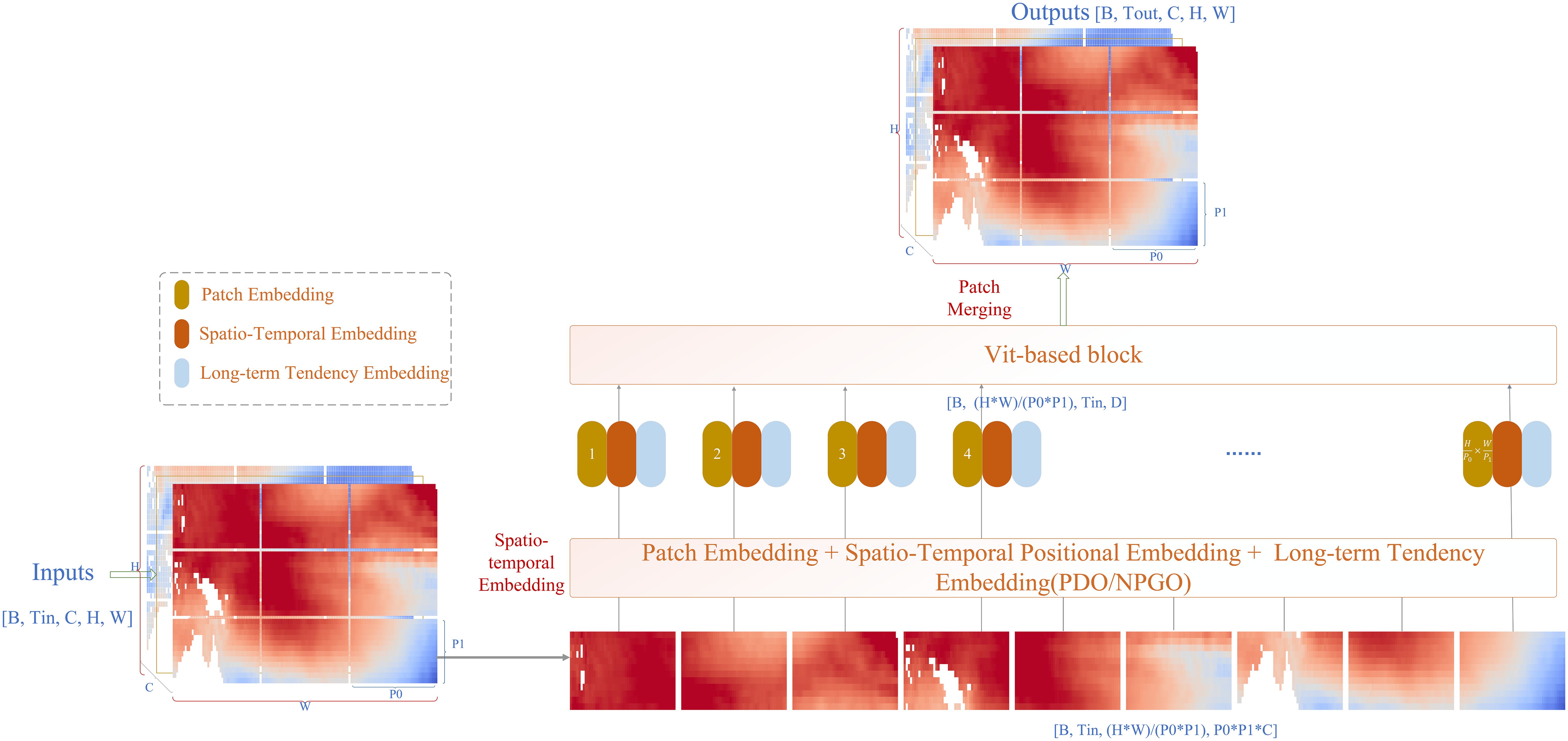
As illustrated in Figure 1, given the ocean parameters input X of dimensions , PGTransNet is trained to forecast the future ocean scenario Y of identical dimensions at a specified lead time . Here, C denotes the number of input features, while H and W represent the latitude and longitude grid points, respectively. and correspond to the input history time step and the output lead time step. In our study, we utilize historical data spanning the previous year to predict temperature and salinity for the subsequent year, where .
PGTransNet relies on several key components to derive the ultimate prediction from historical inputs. These components include data preprocessing, data embedding and merging, revised ViT-based blocks, and physics-guided information integrating. The specific details of each component will be introduced sequentially in the subsequent subsections.
2.2 Datasets and data preprocessing
We utilize the IAP ocean temperature and salinity products from the Institute of Atmospheric Physics (IAP) at the Chinese Academy of Sciences (CAS) Cheng et al. (2017). This dataset is gridded onto a 1° × 1° grid with 41 vertical levels ranging from 1-2000m globally, and monthly resolution spanning from 1940 to the present. The product is developed by using new XBT data bias correction scheme, MBT correction scheme, new reduction of sampling errors scheme (an ensemble optimal interpolation method based on dynamic ensemble samples), and “subsample test” evaluation scheme, which effectively overcomes the problems of large systematic bias and sampling errors. Extensive systematic analysis and evaluation have demonstrated the dataset’s ability to accurately replicate various climate features, including climatological means, decadal variations (such as PDO), interannual variability (such as ENSO), and long-term trends within the historical period from 1940 to 2015, as well as long-term trends Cheng et al. (2017, 2019a, 2019b); Cheng and Zhu (2016); Li et al. (2020). Considering the tropical Pacific Ocean’s pivotal role in the ocean circulation and global climate system, particularly its strong correlation with El Niño and La Niña through changes in upper-ocean temperatures, we specifically select the IAP data over the region spanning from 120°E to 90°W and 20.5°S to 20.5°N, covering the upper-ocean mixed layer from 1 to 160m depths (1, 30, 60, 90, 120, and 160m). We concatenate the salinity and temperature data along the depth dimension, resulting in C = 12. Additionally, it’s worth mentioning that all variations used for predictors and predictands are normalized using min-max normalization within the range [0,1]. The Pacific Decadal Oscillation (PDO) index, as defined by the National Climate Center, serves as the temporal coefficient of the primary mode extracted through empirical orthogonal function (EOF) decomposition of sea surface temperature anomalies within the North Pacific region, spanning from 20°N to 70°N and 110°E to 100°W. This index effectively encapsulates the principal features of large-scale oceanic decadal variability. The cold and warm phases of the PDO index correlate well with the cold and warm anomalies in the tropical Pacific sea surface temperatures, which are strongly associated with many North Pacific and Pacific Northwest climate and ecology records, especially the occurrence of El Niño and La Niña extreme events. Moreover, Liu and Zhu (2015) analyzed the regime shift and its possible causes of winter North Pacific sea surface temperature around the 1990s. The analysis indicates that PDO predominantly influenced the dynamics before 1990, whereas the North Pacific Gyre Oscillation (NPGO) took precedence in the subsequent period. Additionally, it suggests that NPGO is likely to dominate in the future. Therefore, considering the significance of these climate indices in capturing oceanic variability, we propose to embed the first two EOF modes (PDO, NPGO) to alleviate artifacts and strengthen long-term trend forecasting. Notably, according to its definition, the NPGO can be understood as the second EOF mode of sea surface height (SSH) anomalies in the North Pacific. Some studies suggest that the second EOF mode of SST can also approximate the NPGO. Therefore, the NPGO used in this paper is based on the second EOF mode of SST.
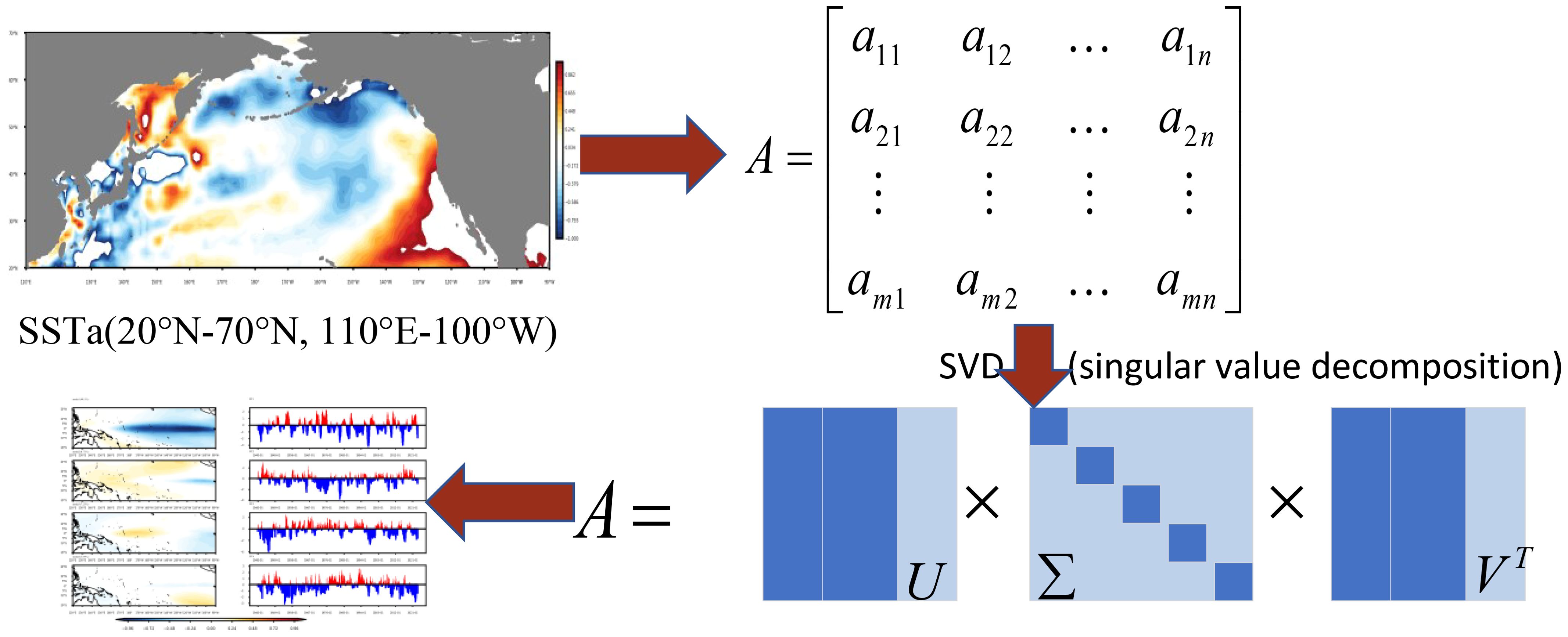
As shown in the Figure 2, EOF decomposes a time-dependent vector field of oceanic variables A (e.g., temperature or salinity) into spatial modes and temporal coefficients, assuming it consists of m spatial points and n time points. In this context, Σ represents the diagonal matrix of singular values, which are the eigenvalues of the covariance matrix of A. Matrix U corresponds to the left singular vector matrix, capturing the spatial patterns, while matrix V represents the right singular vector matrix, reflecting the projection of spatial modes onto the original data matrix A. Essentially, the ith spatial mode is the ith nonzero eigenvector of the covariance matrix of A, and the projection of spatial modes onto the original A corresponds to the respective time coefficients. Table 1 gives the explained variance ratio of the first four modes of the SSTA (SST anomalies) in Pacific. Notably, the cumulative explained variance ratio of the first four modes account over 65%, and the cumulative explained variance ratio of the first two modes over 45%. It is generally believed that the first two modes can basically reflect the main characteristics of the SST variation in this region.
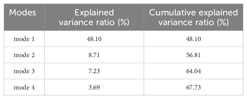
Table 1. The explained variance of the first four modes of EOF decomposition of the Pacific SST anomaly field.
2.3 Data embedding
In our approach, the data undergo several embedding steps before it feed into the model. Firstly, We incorporate patch embedding as a preprocessing step to streamline computational complexity and enhance local feature capture. Inspired by the methodology of ViT, we segment the input data into fixed-size sub-patches and transform each patch into a vector through linear projection.
As depicted in Figure 3, Given an input sample X with shape , and considering a patch size of , we generate a sequence of patches with dimensions , where . For this study, we opt for a patch size of (2, 2), although this parameter can be adjusted based on model performance and computational efficiency considerations. Subsequently, it undergoes linear projection to map it into a specific D-dimensional space.
Secondly, to bolster the model’s temporal and spatial acuity, we introduce spatio-temporal positional encoding and long-term trend embedding into the spatio-temporal embedding process. In this investigation, we employ linear embeddings to convert input tokens into vectors of dimension D, and we evaluate the efficacy of two positional encoding methods within the temporal-positional embedding. One approach utilizes sinusoidal positional encodings, following the methodology proposed by Vaswani Vaswani et al. (2017), while the other incorporates laplacian positional encodings Maskey et al. (2022); Dwivedi et al. (2023). Laplacian encodings represent a natural extension of node position encoding in a graph, based on transformer positional encodings. Leveraging the laplacian eigenvectors facilitates the encoding of relative positional relationships among adjacent graph nodes. Therefore, we explore the integration of laplacian encodings to better capture the spatio-temporal characteristics of neighboring grids within gridded thermodynamic element data. We compute a simple laplacian matrix by subtracting the adjacency matrix from the degree matrix. Subsequently, we utilize the eigenvector with a size of of the laplacian matrix as the position encoding. The long-term decadal variations embedding will be elaborated further in Section 2.5.
2.4 Revised ViT-based block
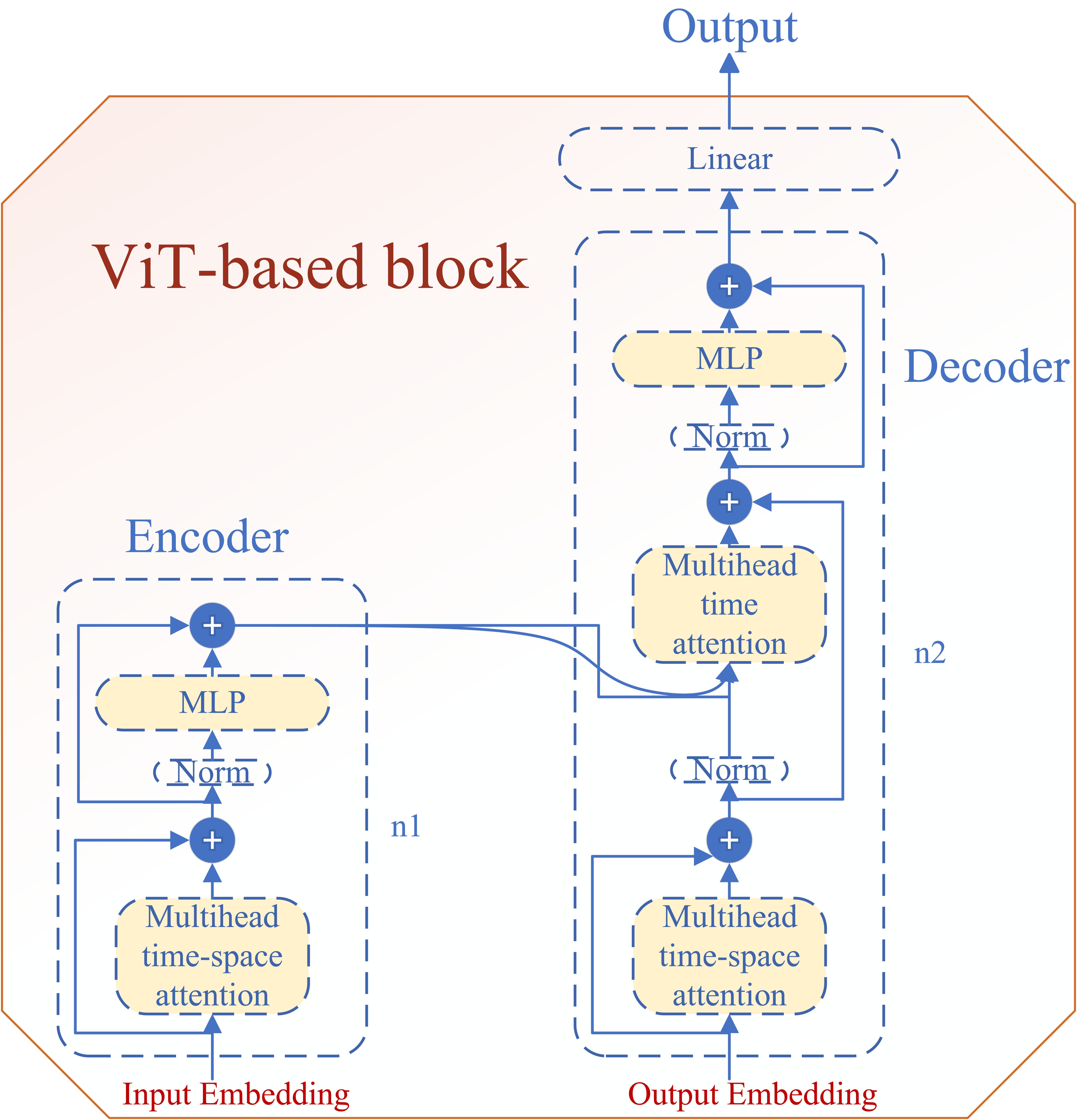
Recently, transformer-based models have emerged as leading contenders for object detection and prediction tasks, often adopting an encoder-decoder architecture. In our study, we leverage a standard transformer encoder-decoder framework with minor adaptations to jointly capture spatio-temporal features of temperature and salinity. As illustrated in Figure 4, the encoder comprises a stack of n1 = 4 identical layers. Each layer incorporates a multi-head time-space attention block with four attention heads and a two-layer MLP block with a ReLU non-linearity, facilitating the aggregation of spatial-temporal features and physical information. Drawing inspiration from the efficiency of the ViT transformer in computational resource-saving, we feed the resulting sequence of linear embeddings of the fixed-size patches after patch embedding into the encoder. Meanwhile, the decoder consists of a stack of n2 = 4 identical layers. In contrast to the encoder, the decoder focuses on multi-head time attention concerning the output from the encoder stack.
2.5 Physics-guided information integrating
Next, we elucidate our approach on how we incorporating physics information into the model. This integration encompasses three facets: long-term dynamics embedding, the imposition of soft constraints based on the thermodynamic equation, and the restriction of the output solution space. We make linear PDO or NPGO embedding to capture long-term dynamics. As detailed in Section 2.2, the PDO index effectively characterizes large-scale oceanic decadal variations, serving as the temporal coefficient of the primary mode obtained from EOF analysis. It manifests as a one-dimensional time series, encapsulating the principal features of such variations. Henceforth, we augment the dimension of the PDO index and integrate it with the input data through linear aggregation. A similar procedure is employed for processing the NPGO. Subsequently, we incorporated the thermodynamic properties of seawater (specifically, density) into the model in a soft-constraint manner to guide the model’s output to match a specific thermohaline density relationship. It is worth noting that the thermodynamic equation used to calculate density is based on the latest seawater thermodynamic calculation standard TEOS-10. TEOS-10 supersedes the former standard EOS-80 (Equation of State of Seawater, 1980; International Association for the Properties of Water and Steam, 2018), and it provides a comprehensive, thermodynamically consistent manner for all thermodynamic properties of seawater (density, enthalpy, entropy sound speed, etc.) based on Gibbs function (named after Josiah Willard Gibbs) formulation. This primer Pawlowicz (2010) points out that all thermodynamic properties of the system can be determined by specific combinations of derivatives of the Gibbs function. So the key to solving the seawater problem becomes how one compute the Gibbs function for seawater. TEOS-10 defines the Gibbs function of seawater as the sum of a pure water gW part and the saline part gS (IAPWS-08), Commission et al. (2010). Concretely, the density of seawater ρ is determined by the reciprocal of the pressure derivative of the Gibbs function (g) at constant absolute salinity (SA) and in situ temperature T. Specifically,
where, , and P means sea pressure. Besides, it’s noteworthy that all the equations to calculate thermodynamic properties were integrated into the open source Gibbs-Seawater (GSW) Oceanographic Toolbox McDougall and Barker (2011). Consequently, we call the function gsw_rho_t_exact(SA,T,P) that computes the density in this tool directly [for more information about this, please refer to Commission et al. (2010)].
Given the prediction and the ground truth Y, the combined loss is formulated as follows:
Where,
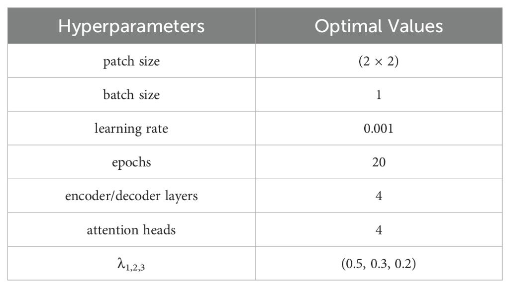
In our formulation, Loss denotes a composite temperature-salinity loss, wherein and represent the independent losses for temperature and salinity, respectively. Additionally, signifies the density loss, which is computed based on the model’s temperature and salinity outputs using the TEOS-10 equation. The calculation formula for and mirrors that of . Furthermore, , , and denote adaptive hyperparameters, with an optimal combination typically being (0.5, 0.3, 0.2). Finally, considering the range of temperature and salinity values, we incorporated a constraint layer to confine them within a predetermined range, thus ensuring adherence to fundamental physical laws.
As for the output solution space restriction, we sought to limit the model’s output by applying the maximum and minimum ranges of temperature and salinity consistent with the TEOS-10 equation . These constraints were standardized alongside the data. To mitigate the impact of normalization, we conducted ablation experiments by directly inputting the raw temperature and salinity data into the model, applying the original scale constraints accordingly. Regardless of whether the data were standardized or not, our experiments revealed no enhancement in the model’s forecasting performance upon integrating these constraint ranges. This outcome suggests that the ranges may have been overly broad, surpassing the actual extremities of temperature and salinity within the studied area. Future endeavors could focus on pinpointing more precise ranges based on genuine environmental conditions.
3 Experiments and results
3.1 Experimental settings
We conduct extensive experiments using temperature and salinity data in the tropical Pacific from January 1940 to September 2023. The model training is conducted on a server equipped with a TESLA-V100 GPU with 16GB memory. Detailed model parameters are provided in Table 2.
3.2 Baseline and evaluation metrics
In this section, we consider the following CNN-based, ConvLSTM-based, and TransNet as baseline. TransNet is the backbone of PGTransNet which does not contain any physical information, but is a modified version of ViT Dosovitskiy et al. (2020). Figures 5 and 6 give the competitive model based on CNN and ConvLSTM, both the prediction models have been trained with a batch size of 8 and kernel size (2,2) or (2,2,2) by adaptive momentum (Adam) with an initial learning rate of 0.001 for 30 epochs, and the learning rate is adjusted using the ReduceLROnPlateau mode.
Besides, we use the following evaluation metrics to measure the performance of different methods:
1. Root mean square error (RMSE); It is used to measure the deviation of computed values concerning observed ones.
2. Anomaly correlation coefficient (ACC); It quantifies the correlation between anomalies of predicted values and validation values (ground truth):
3. Bias/Mean Bias. We employ Bias to gauge the positive and negative deviations between grids, and Mean Bias to quantifies the disparity between the spatial mean of the prediction and the spatial mean of the ground truth.
For all metrics, we denote and Y as the prediction and ground truth, which have a shape of , where N is the number of test samples, C refers to the depth channel, is the spatial resolution.
3.3 Quantitative evaluation results
3.3.1 Overall performance
To comprehensively evaluate the performance of PGTransNet, we utilize 12 consecutive months of historical data to forecast temperature and salinity for the subsequent 12 months. We conducted ablation experiments to perform a sensitivity analysis and evaluate the effectiveness of each module in the model based on various validation factors. Figure 7 presents the averaged RMSE and ACC over the forecasting times of the baseline model alongside the augmented model with progressively integrated physical information modules.
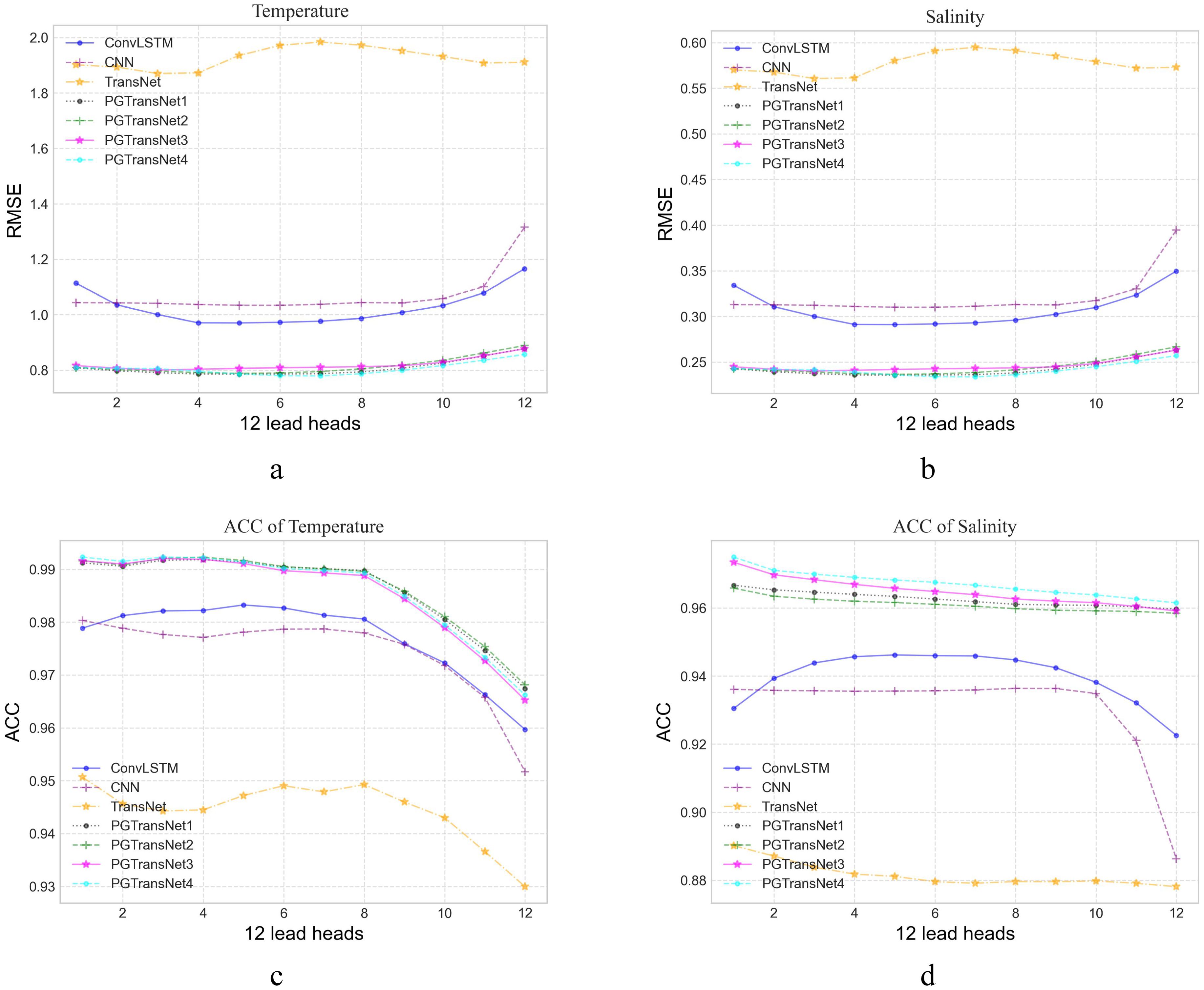
Figure 7. The PGTransNet performance on tropical Pacific forecasting, and its comparison against other ablation models. (A) RMSE of temperature; (B) RMSE of salinity; (C) ACC of temperature; (D) ACC of salinity.
Figure 7 presents the performance of each model in terms of RMSE and ACC. Specifically, TransNet is the modified version of ViT as mentioned above, PGTransNet_PDO represents TransNet augmented with combine loss of temperature, salinity and density, and PDO long-term decadal variations embedding. PGTransNet_NPGO further incorporates NPGO embedding on top of PGTransNet_PDO. PGTransNet_PDO_Laplacian integrates laplacian encodings on top of PGTransNet_PDO, and PGTransNet_NPGO_Laplacian integrates laplacian encodings on top of PGTransNet_NPGO. For brevity, we denote PGTransNet_PDO, PGTransNet_NPGO, PGTransNet_PDO_Laplacian, and PGTransNet_NPGO_Laplacian as PGTransNet1, PGTransNet2, PGTransNet3, and PGTransNet4 in the diagram, respectively. All of these models belong to the PGTransNet group.
The x-axis and y-axis denote the forecast time and the corresponding forecasting RMSE/ACC, respectively. Lower RMSE and higher ACC values indicate better model performance and prediction accuracy. From Figure 7, it’s evident that the PGTransNet group outperforms the CNN-based and ConvLSTM-based models in both temperature and salinity forecasting. Surprisingly, the ViT-based backbone TransNet, which lacks incorporation of any physical laws, performs the worst. We observe that while TransNet achieves an accuracy of 0.99 on the training set, it yields an RMSE of 1.932 on the test set. Embedding decadal variability and the thermodynamic equation into the model significantly improves prediction accuracy on the test set by over 40%. This highlights the robustness and generalization capabilities of PGTransNet in forecasting. Moreover, ablation experiments involving the incremental addition of PDO, NPGO, and laplacian encodings reveal that all these physics-guided models achieve comparable performance. The benefits of incorporating various physical information and embedding the laplacian encodings are evident in mitigating prediction biases in coastal and marginal sea regions, and improving prediction accuracy in high-temperature areas at different vertical depths. For further details, refer to Section 3.4.1.
Additionally, we present the average performance of the aforementioned models across all test samples (averaged from January 2020 to September 2023) in Table 3. It can be observed that our physics-guided model outperforms the baseline model in terms of temperature and salinity forecasting, and all models achieve comparable performance.
3.3.2 Temperature/salinity profiles evaluation
To comprehensively assess the model’s forecasting ability in the vertical direction, Figure 8 presents the average RMSE in vertical temperature and salinity profiles for different models within the upper 160 meters (at depths of 1, 20, 50, 80, 120, and 160 meters, latitude=0°).
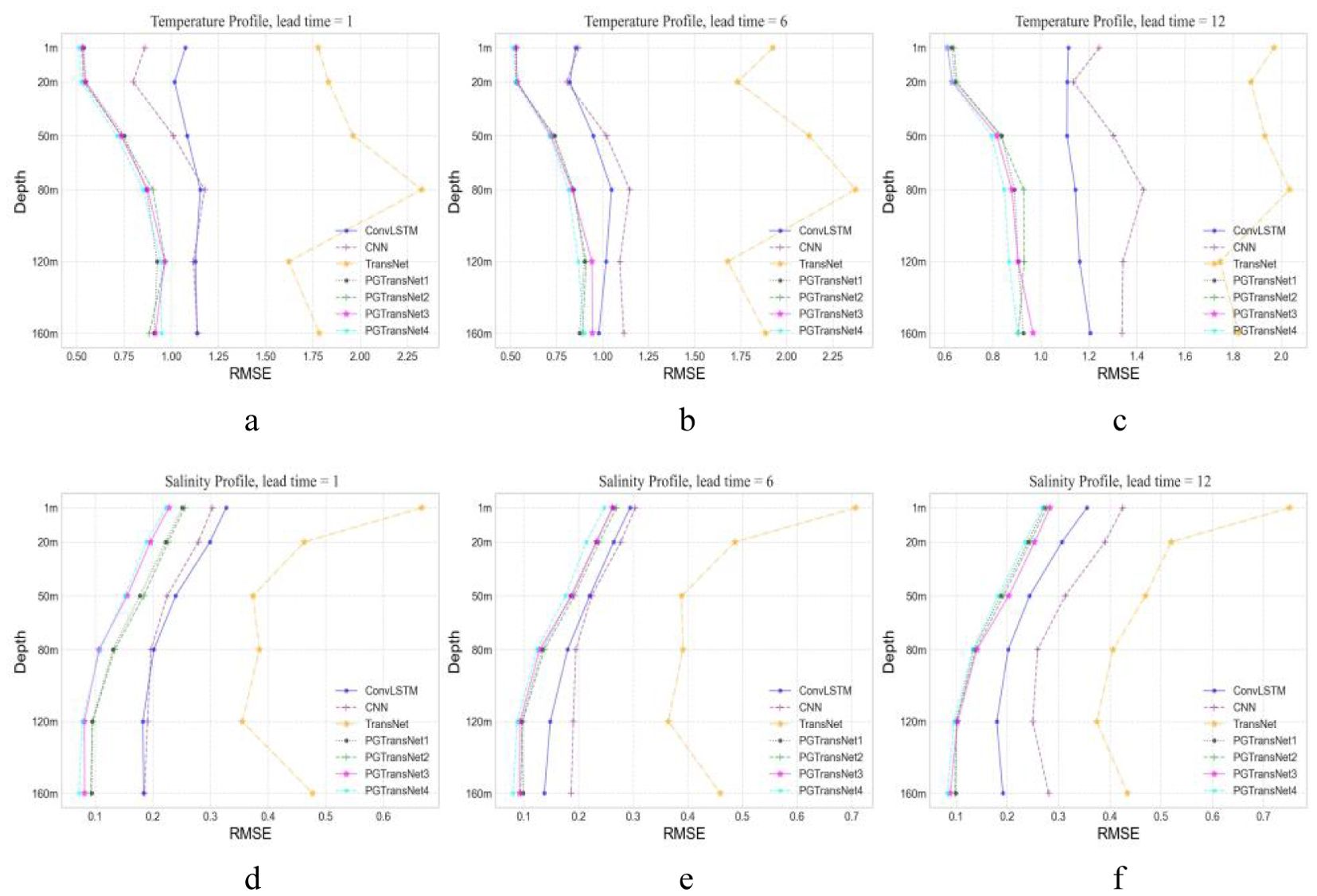
Figure 8. The profiles of temperature and salinity RMSE above 160m for different models at lead time = (1, 6, 12). The reported RMSE is averaged from Jan. 2020 to Sep. 2023. (A) RMSE of temperature profile (lead time = 1); (B) RMSE of temperature profile (lead time = 6); (C) RMSE of temperature profile (lead time = 12); (D) RMSE of salinity profile (lead time = 1); (E) RMSE of salinity profile (lead time = 6); (F) RMSE of salinity profile (lead time = 12).
Figure 8 illustrates that the physics-guided PGTransNet model group outperforms the baseline model significantly. For salinity prediction, PGTransNet4, which incorporates PDO, NPGO, and laplacian positional encoding, notably performs better than the others. Except for TransNet, the RMSE decreases with increasing depth for other models. For temperature prediction, PGTransNet4 demonstrates the best performance overall. However, from the temperature profile curve, the predictions at lead times 1 and 6 are slightly inferior to the other models in the PGTransNet group at a depth of 160m. Nonetheless, this model exhibits better forecasting performance for sea surface temperature. As the depth increases, the model’s forecasting accuracy for underwater temperature deteriorates, leading to higher RMSE values. Besides, it is evident that for both temperature and salinity profiles, the ViT-based TransNet exhibits the largest RMSE, even worse than the CNN-based and ConvLSTM-based models. This is attributed to the overfitting issue mentioned earlier, leading to a deterioration in performance on the test set.
3.4 Cases study for visualization
3.4.1 Predictions and bias
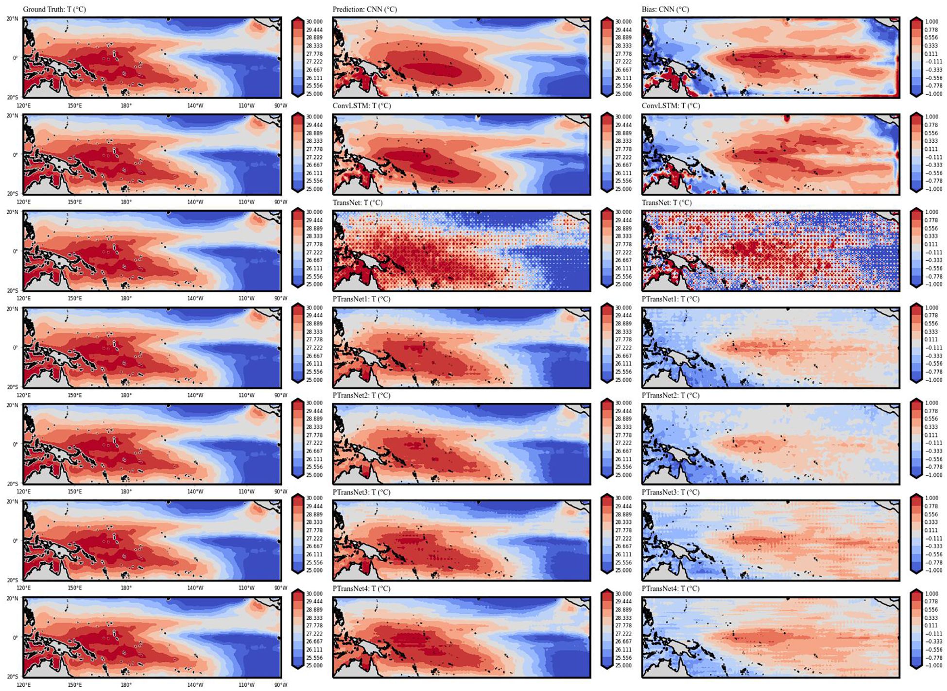
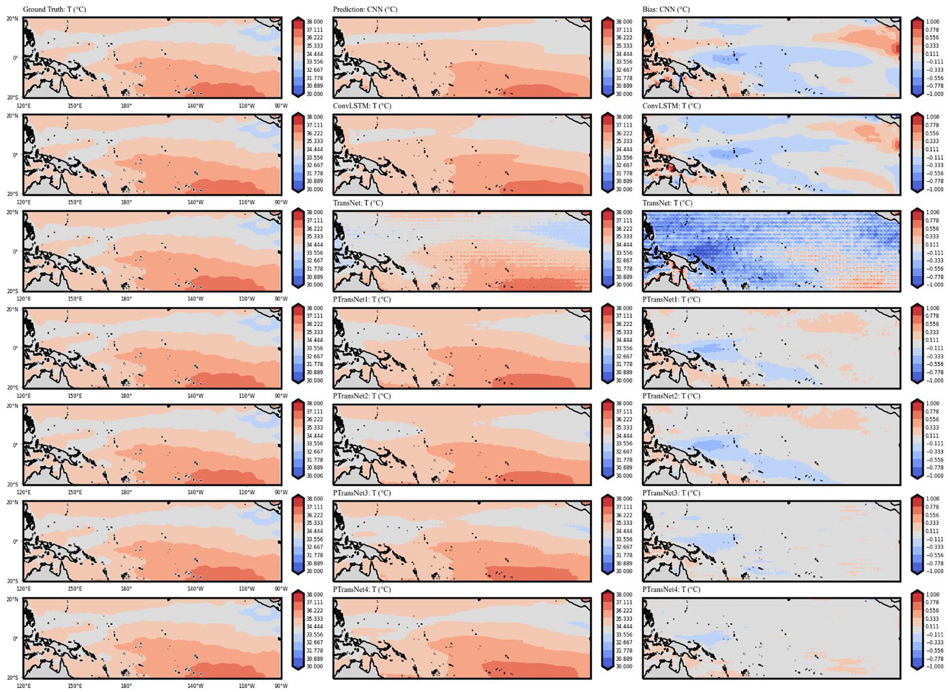
Figures 9 and 10 visualizes the ground truth, predictions and bias of these model for the temperature and salinity. The first column of the graph represents the ground truth, displaying actual values. The second column represents the predicted values of each ablation model. Finally, the third column illustrates the bias between the predicted values of each ablation model and the ground truth.
For sea surface temperature prediction, the graph illustrates that all models effectively capture the large-scale distribution of sea surface temperature in the tropical pacific region except TransNet. It is obvious that all the models within the PGTransNet group can learn a better distribution than CNN-based and ConvLSTM-based model. Comparing the distribution of sea surface temperature ground truth and predictions, PGTransNet4, which integrates PDO, NPGO, and laplacian encodings, can better captures the high-temperature center region with just a slight overestimation. PGTransNet2 exhibits lower bias in regions with relatively lower temperatures. Additionally, from the bias, it can be observed that PGTransNet4 has lower bias in the gulf and nearshore areas. Regarding salinity prediction, all the models demonstrate the capability to capture the large-scale distribution characteristics in the tropical pacific region except TransNet. In general, PGTransNet4 has the best performance.
3.4.2 ACC distribution
To clearly assess the model’s forecasting performance across oceanic geographical space, we present the spatial distribution of anomaly correlation coefficient (ACC). As shown in the Figure 11, the physics-guided PGTransNet group exhibits higher forecasting accuracy in coastal and marginal sea areas compared to the baseline TransNet, CNN-based and ConvLSTM-based model. Whether only adding PDO or further incorporating laplacian encoding on top of it, the effect is quite satisfactory.
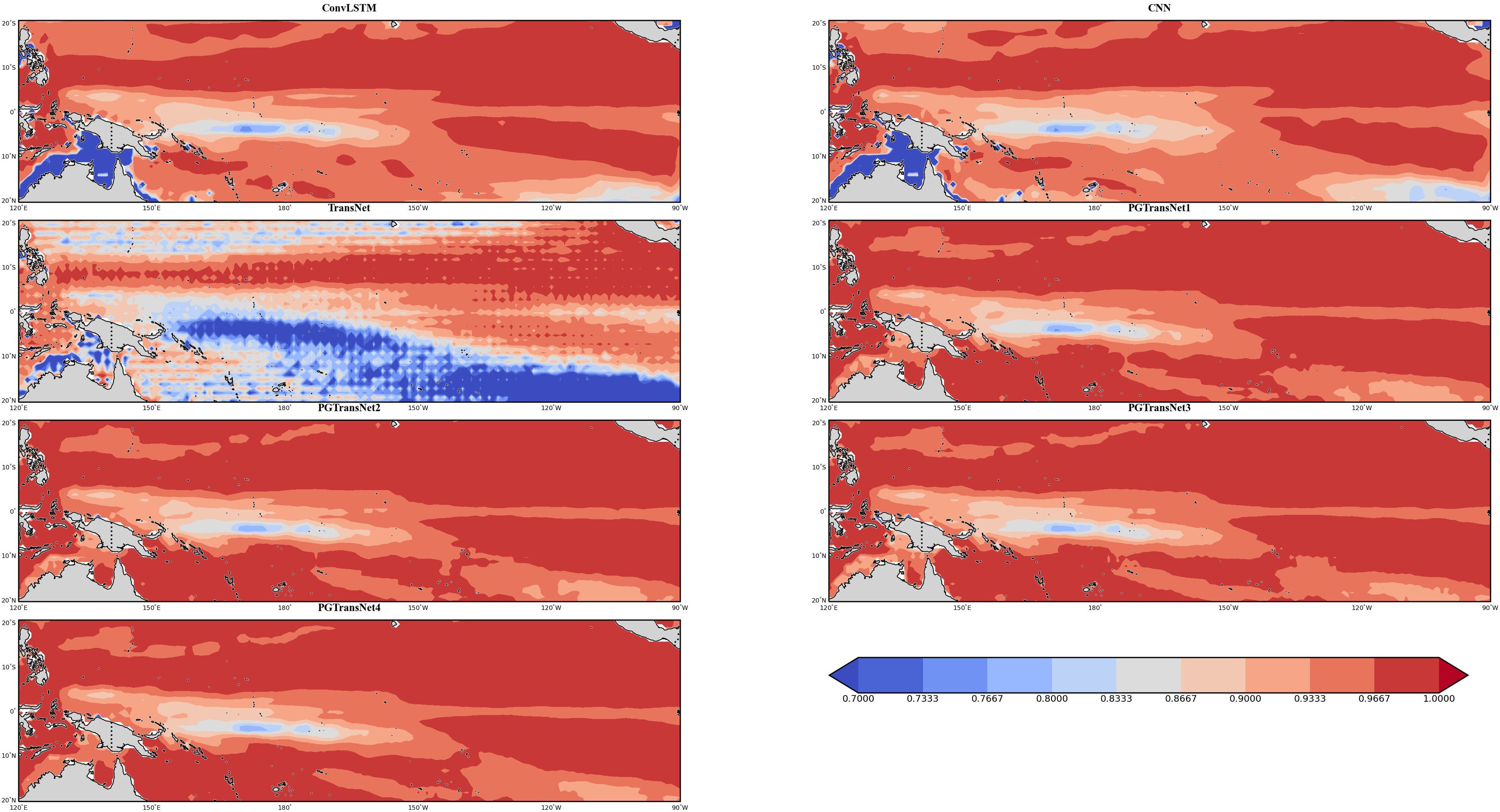
Figure 11. Distributions of the ACCs among all models calculated between analyzed and predicted fields during Jan. 2020 to Sep. 2023.
3.5 Parameter insensitivity analysis
During model training, we found that without adding any physical information, inappropriate hyperparameter adjustments can easily lead to overfitting or underfitting. For instance, when the patch size and batch size are both small (e.g. p = 2×2, batchsize = 1), TransNet can achieve an accuracy of 0.99 on the training set. However, the RMSE on the test set is 1.932, indicating poor performance in predicting the large-scale temperature distribution. In contrast, our model can achieve comparable forecasting accuracy as long as the parameters are within a reasonable range, regardless of how small they are set.
3.6 Physical consistency analysis
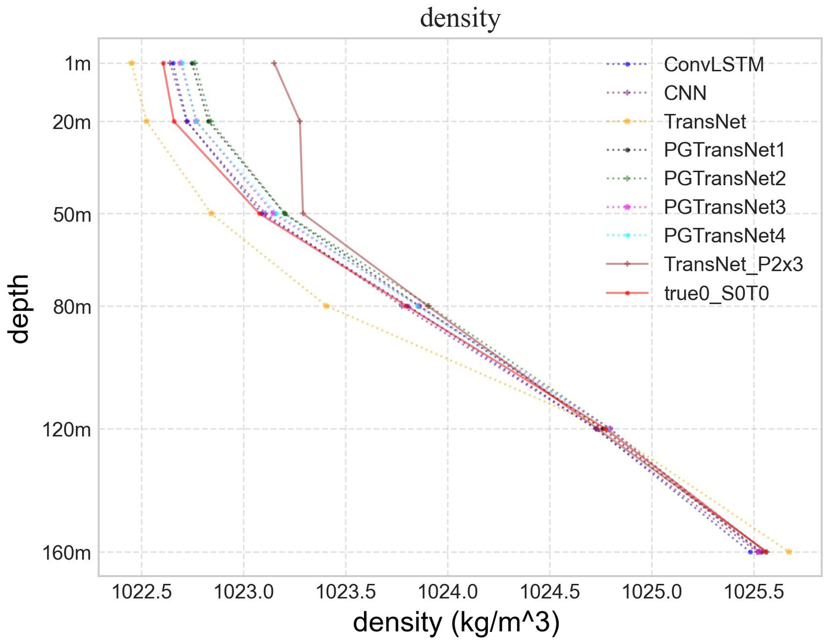
Under normal circumstances, the density of the upper ocean mixed layer increases gradually with depth. The density of lower seawater is greater than that of upper seawater, exhibiting a monotonic behavior. Therefore, based on the TEOS-10 thermodynamic equation, we calculate the corresponding ocean density values from the temperature and salinity data predicted by the model. Figure 12 present the density profiles mean values for the entire study area in January 2020, under the parameter settings described earlier, the densities of all models satisfy the monotonicity condition. However, during the training and parameter tuning process, we find that although the backbone model TransNet performs well on the training set, its performance on the test dataset is poor, under certain parameter conditions (e.g. batchsize = 2,patchsize = 2 × 3), there are occasional instances of density values deviating abnormally, as indicated by the solid brown line the Figure 12.
3.7 Generality analysis
To further analyze the generalization capability of the model, we conduct temperature and salinity forecasting for two localized regions at the Earth’s northern and southern extremes. Region 1: part of the Arctic Ocean, with a latitude range of [66.5°N, 89.5°N] and a longitude range of [1°E, 40°E]. Region 2: latitude range [29°S, 69°S] and longitude range [25°W, 85°W]. Region 1 is selected to assess the effect of the model on the prediction of ocean temperature and salinity in the polar region. Region 2 is chosen because its latitude spans high, medium, and low latitudes, and geographically, it encompasses parts of South America, the Antarctic Peninsula, and the South Shetland Islands. This ensures that the study area includes various complex spatial topographical variations in ocean temperature, allowing for a more comprehensive evaluation of the proposed model’s capabilities. Figure 13 presents the performance of sea surface temperature forecasting for Region 1. The distribution is similar to that shown in Figure 9. From the figure, it is evident that the PGTransNet_PDO model outperforms other models, indicating that our proposed method achieves superior forecasting performance even in polar regions.
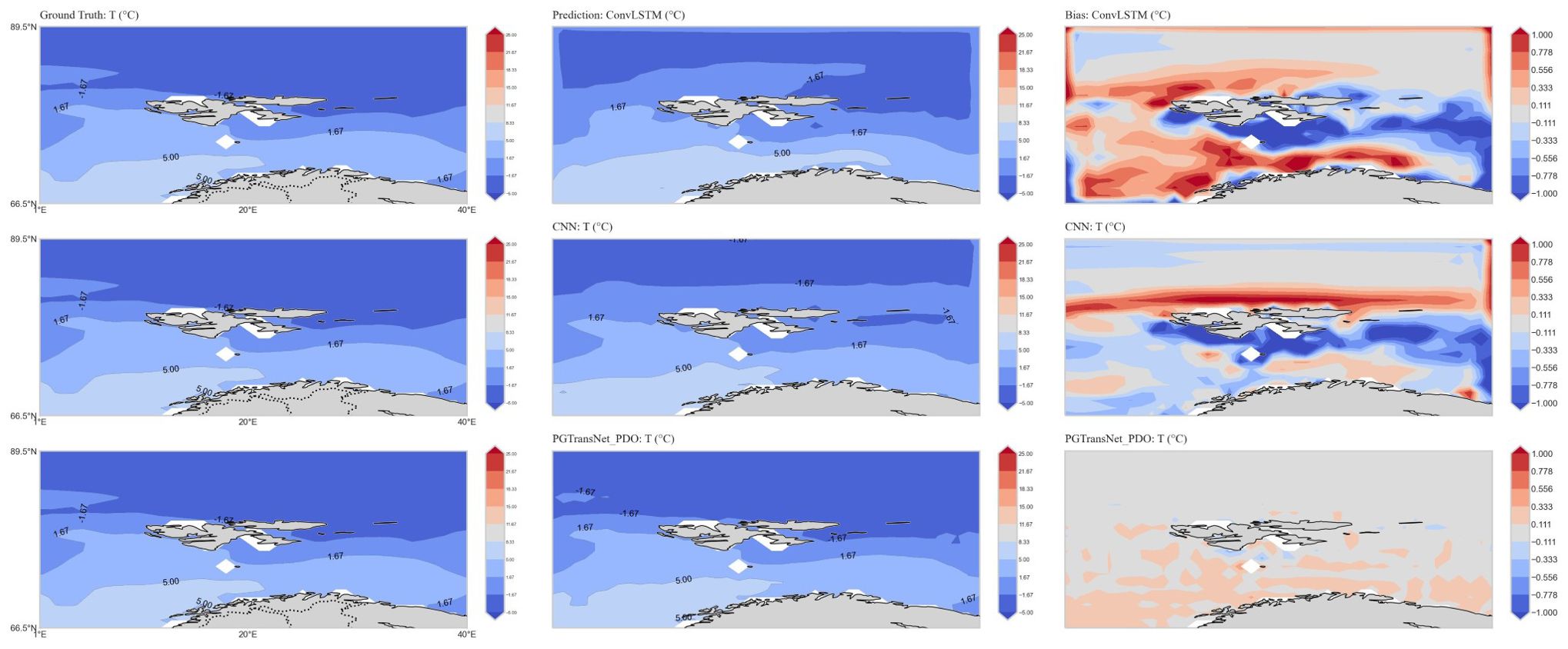
Figure 13. Generality analysis: example visualizations of temperature prediction by CNN, ConvLSTM ans PGTransNet_PDO in Region 1 (Depth=1m, Jan. 2020).
Figure 14 shows the sea surface temperature forecasting results for Region 2 during spring (March). We can see from the picture that the overall bias of the ConvLSTM and CNN models is significantly higher than that of PGTransNet_PDO, especially in coastal and nearshore areas. The biases of the two baseline models are significantly higher, possibly because the ocean environment in coastal and nearshore regions is heavily influenced by topography. Additionally, at the boundary between land and sea, geographical features such as ocean currents and tides affect the movement of water bodies and temperature distribution, thereby increasing the complexity of forecasting. In contrast, PGTransNet_PDO exhibits a lower bias in coastal and nearshore areas, indicating that PGTransNet_PDO demonstrates superior forecasting performance and greater model robustness.
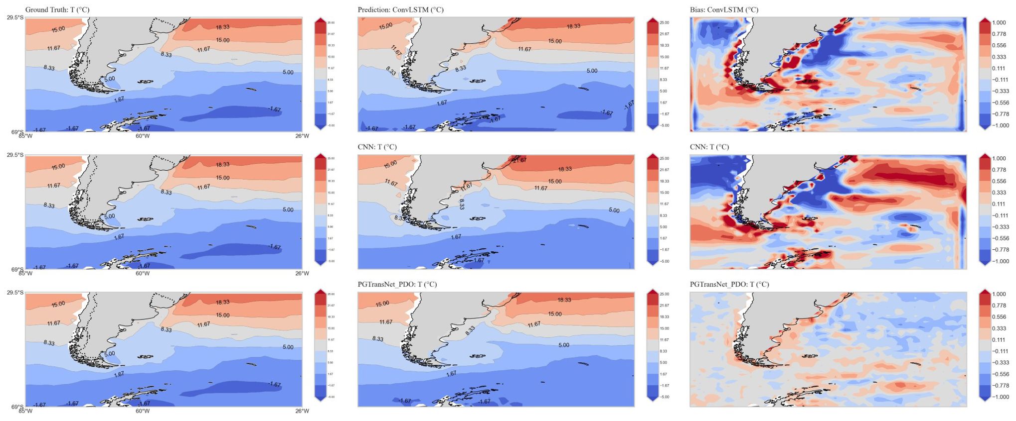
Figure 14. Generality analysis: example visualizations of temperature prediction by CNN, ConvLSTM ans PGTransNet_PDO in Region 2 (Depth=1m, Mar. 2020).
4 Conclusions
In this paper, we propose a novel physics-guided spatio-temporal self-attention hybrid network PGTransNet for temperature and salinity jointly forecasting in the Tropical Pacific. Compared with the benchmark model without physical knowledge, the PGTransNet group can obtain higher prediction accuracy. Extensive experiments and visualizations show that our model is insensitive to hyperparameter tuning, ensuring both better generalization and physical consistency. Moreover, as observed from the spatial distribution of anomaly correlation coefficient, the model exhibits higher forecasting accuracy for coastal and marginal sea regions.
As for the output solution space restriction, it confine the temperature-salinity outputs within a specific range. Since the TEOS-10 provides a broad range of constraint values, which are generally applicable to the outputs, they do not significantly affect the model results. Subsequent refinements of the constraint values can be made based on specific circumstances.
From the Figures 9 and 10, it is evident that high biases occur in the central equatorial Pacific region. We know that this anomalous area aligns with wind-driven circulation. Ocean circulation is influenced by wind stress, heat flux, and water flux acting together, with different factors dominating in different scenarios. In the future, we will incorporate sea surface zonal and meridional wind stress as input features, and embedding ocean heat flux information and other relevant data into the model to guide model training and improve predictions in anomalous marine areas.
Data availability statement
The original contributions presented in the study are included in the article/supplementary material. Further inquiries can be directed to the corresponding authors.
Author contributions
SW: Formal analysis, Methodology, Visualization, Writing – original draft, Writing – review & editing, Conceptualization, Data curation, Software, Validation. SB: Conceptualization, Investigation, Methodology, Validation, Writing – review & editing. WD: Funding acquisition, Methodology, Resources, Writing – review & editing. SZW: Conceptualization, Methodology, Writing – review & editing. XZ: Methodology, Resources, Writing – review & editing. CS: Supervision, Writing – review & editing. JZ: Formal analysis, Methodology, Writing – review & editing. XL: Conceptualization, Funding acquisition, Project administration, Resources, Writing – review & editing.
Funding
The author(s) declare financial support was received for the research, authorship, and/or publication of this article. This work is supported by the National Natural Science Foundation of China (Grant Nos. 42275170, 62032019, 42305170, 62202487, 62402512), the Science and Technology Innovation Program of Hunan Province (2022RC3070), the National Key R&D Program of China (2021YFC3101502), the Natural Science Foundation of Hunan Province (Grant No. 2023JJ40678), and the Scientific Research Program of the National University of Defense Technology (No. ZK22-13).
Acknowledgments
The dataset was provided by the Chinese Academy of Sciences (CAS). Thanks to all the members for their help.
Conflict of interest
The authors declare that the research was conducted in the absence of any commercial or financial relationships that could be construed as a potential conflict of interest.
Publisher’s note
All claims expressed in this article are solely those of the authors and do not necessarily represent those of their affiliated organizations, or those of the publisher, the editors and the reviewers. Any product that may be evaluated in this article, or claim that may be made by its manufacturer, is not guaranteed or endorsed by the publisher.
References
Aguilar-Martinez S., Hsieh W. W. (2009). Forecasts of tropical pacific sea surface temperatures by neural networks and support vector regression. Int. J. Oceanogr. 1, 167239. doi: 10.1155/2009/167239
Chen Q., Cai C., Chen Y., Zhou X., Zhang D., Peng Y. (2024). Tempronet: A transformer-based deep learning model for seawater temperature prediction. Ocean Eng. 293, 116651. doi: 10.1016/j.oceaneng.2023.116651
Cheng L., Abraham J., Hausfather Z., Trenberth K. E. (2019a). How fast are the oceans warming? Science 363, 128–129. doi: 10.1126/science.aav7619
Cheng L., Trenberth K. E., Fasullo J., Boyer T., Abraham J., Zhu J. (2017). Improved estimates of ocean heat content from 1960 to 2015. Sci. Adv. 3, e1601545. doi: 10.1126/sciadv.1601545
Cheng L., Trenberth K. E., Fasullo J. T., Mayer M., Balmaseda M., Zhu J. (2019b). Evolution of ocean heat content related to enso. J. Climate 32, 3529–3556. doi: 10.1175/JCLI-D-18-0607.1
Cheng L., Zhu J. (2016). Benefits of cmip5 multimodel ensemble in reconstructing historical ocean subsurface temperature variations. J. Climate 29, 5393–5416. doi: 10.1175/JCLI-D-15-0730.1
Commission, I. O., on Oceanic Research, S. C., and for the Physical Sciences of the Oceans, I. A (2010). The International Thermodynamic Equation of Seawater – 2010: Calculation and Use of Thermodynamic Properties (Paris).
Dai H., He Z., Wei G., Lei F., Zhang X., Zhang W., et al. (2024). Long-term prediction of sea surface temperature by temporal embedding transformer with attention distilling and partial stacked connection. IEEE J. Select. Topics Appl. Earth Observ. Remote Sens. 17, 4280–4293. doi: 10.1109/JSTARS.2024.3357191
Daw A., Thomas R. Q., Carey C. C., Read J. S., Appling A. P., Karpatne A. (2020). “Physics-guided architecture (pga) of neural networks for quantifying uncertainty in lake temperature modeling,” in Proceedings of the 2020 SIAM International Conference on Data Mining (SDM). Society for Industrial and Applied Mathematics, 532–540.
Daw A., Karpatne A., Watkins W. D., Read J. S., Kumar V. (2017). Physics-guided neural networks (pgnn): An application in lake temperature modeling. In Knowledge Guided Machine Learning, 353–372. Chapman and Hall/CRC.doi: 10.1201/9781003143376-15
Dosovitskiy A., Beyer L., Kolesnikov A., Weissenborn D., Zhai X., Unterthiner T., et al. (2020). An image is worth 16x16 words: Transformers for image recognition at scale. arXiv preprint arXiv:2010.11929. doi: 10.48550/arXiv.2010.11929
Dwivedi V. P., Joshi C. K., Luu A. T., Laurent T., Bengio Y., Bresson X. (2023). Benchmarking graph neural networks. J. Mach. Learn. Res. 24, 1–48.
Fischer C. C., Tibbetts K. J., Morgan D., Ceder G. (2006). Predicting crystal structure by merging data mining with quantum mechanics. Nat. materials 5, 641–646. doi: 10.1038/nmat1691
Hou S., Li W., Liu T., Zhou S., Guan J., Qin R., et al. (2022). Must: A multi-source spatio-temporal data fusion model for short-term sea surface temperature prediction. Ocean Eng. 259, 111932. doi: 10.1016/j.oceaneng.2022.111932
International Association for the Properties of Water and Steam, IAPWS R6-95(2018), Revised Release on the IAPWS Formulation 1995 for the Thermodynamic Properties of Ordinary Water Substance for General and Scientific Use (2018).
Jia X., Willard J., Karpatne A., Read J. S., Zwart J. A., Steinbach M., et al. (2021). Physics-guided machine learning for scientific discovery: An application in simulating lake temperature profiles. ACM/IMS Trans. Data Sci. 2, 1–26. doi: 10.1145/3447814
Jiang C. M., Kashinath K., Prabhat, Marcus P. (2019). “Enforcing physical constraints in CNNs through differentiable PDE layer,” in ICLR 2020 Workshop on Integration of Deep Neural Models and Differential Equations.
Kug J.-S., Kang I.-S., Lee J.-Y., Jhun J.-G. (2004). A statistical approach to Indian ocean sea surface temperature prediction using a dynamical enso prediction. Geophys. Res. Lett. 31. doi: 10.1029/2003GL019209
Li G., Cheng L., Zhu J., Trenberth K. E., Mann M. E., Abraham J. P. (2020). Increasing ocean stratification over the past half-century. Nat. Climate Change 10, 1116–1123. doi: 10.1038/s41558-020-00918-2
Lin L., Zhang Z., Yu H., Wang J., Gao S., Zhao H., et al. (2024). Sthcformer: Amultivariate ocean weather predicting method based on spatiotemporal hybridconvolutional attention networks. IEEE J. Select. Topics Appl. Earth Observ. Remote Sens. 17, 3600–3614. doi: 10.1109/JSTARS.2024.3354254
Liu K., Zhu C. (2015). Regime shift of winter north pacific sea surface temperature after 1990 and its possible causes. Chin. J. Atmos. Sci. (in Chinese) 39, 926–940.
Maskey S., Parviz A., Thiessen M., Stärk H., Sadikaj Y., Maron H. (2022). Generalized laplacian positional encoding for graph representation learning. arXivpreprint. doi: 10.48550/arXiv.2210.15956
McDougall T. J., Barker P. M. (2011). Getting started with teos-10 and the gibbs seawater (gsw) oceanographic toolbox. Scor/iapso WG 127, 1–28.
Patil K., Deo M., Ravichandran M. (2016). Prediction of sea surface temperature by combining numerical and neural techniques. J. Atmos. Ocean. Technol. 33, 1715–1726. doi: 10.1175/JTECH-D-15-0213.1
Patil K. R., Iiyama M. (2021). “Deep neural networks to predict sub-surface ocean temperatures from satellite-derived surface ocean parameters,” in Soft Computing for Problem Solving: Proceedings of SocProS 2020, Vol. 2. 423–434 (Springer).
Qiao B., Wu Z., Ma L., Zhou Y., Sun Y. (2023). Effective ensemble learning approach for sst field prediction using attention-based predrnn. Front. Comput. Sci. 17, 171601. doi: 10.1007/s11704-021-1080-7
Song T., Wang Z., Xie P., Han N., Jiang J., Xu D. (2020). A novel dual path gated recurrent unit model for sea surface salinity prediction. J. Atmos. Ocean. Technol. 37, 317–325. doi: 10.1175/JTECH-D-19-0168.1
Vaswani A., Shazeer N., Parmar N., Uszkoreit J., Jones L., Gomez A. N., et al. (2017). Attention is all you need. Adv. Neural Inf. Process. Syst. 30.
Von Rueden L., Mayer S., Beckh K., Georgiev B., Giesselbach S., Heese R., et al. (2021). Informed machine learning–a taxonomy and survey of integrating prior knowledge into learning systems. IEEE Trans. Knowledge Data Eng. 35, 614–633. doi: 10.1109/TKDE.69
Wang H., Hu S., Li X. (2023). An interpretable deep learning enso forecasting model. Ocean-Land-Atmos. Res. 2, 0012. doi: 10.34133/olar.0012
Wu D., Gao L., Xiong X., Chinazzi M., Vespignani A., Ma Y.-A., et al. (2021). Deepgleam: a hybrid mechanistic and deep learning model for covid-19 forecasting. arXiv preprint. doi: arXiv:2102.06684
Wu S., Zhang X., Bao S., Dong W., Wang S., Li X. (2023). Predicting ocean temperature in high-frequency internal wave area with physics-guided deep learning: A case study from the south China sea. J. Mar. Sci. Eng. 11, 1728. doi: 10.3390/jmse11091728
Xiao C., Chen N., Hu C., Wang K., Xu Z., Cai Y., et al. (2019). A spatiotemporal deep learning model for sea surface temperature field prediction using time-series satellite data. Environ. Model. Softw. 120, 104502. doi: 10.1016/j.envsoft.2019.104502
Xiao C., Tong X., Li D., Chen X., Yang Q., Xv X., et al. (2022). Prediction of long lead monthly three-dimensional ocean temperature using time series gridded argo data and a deep learning method. Int. J. Appl. Earth Observ. Geoinform. 112, 102971. doi: 10.1016/j.jag.2022.102971
Xu L., Li Q., Yu J., Wang L., Xie J., Shi S. (2020). Spatio-temporal predictions of sst time series in China’s offshore waters using a regional convolution long short-term memory (rc-lstm) network. Int. J. Remote Sens. 41, 3368–3389. doi: 10.1080/01431161.2019.1701724
Yuan T., Zhu J., Ren K., Wang W., Wang X., Li X. (2022). “Neural network driven by space-time partial differential equation for predicting sea surface temperature,” in 2022 IEEE International Conference on Data Mining (ICDM). Orlando, FL, USA: IEEE, 656–665. doi: 10.1109/ICDM54844.2022.00076
Zhang Q., Wang H., Dong J., Zhong G., Sun X. (2017). Prediction of sea surface temperature using long short-term memory. IEEE Geosci. Remote Sens. Lett. 14, 1745–1749. doi: 10.1109/LGRS.2017.2733548
Zhou L., Zhang R.-H. (2023). A self-attention–based neural network for three-dimensional multivariate modeling and its skillful enso predictions. Sci. Adv. 9, eadf2827. doi: 10.1126/sciadv.adf2827
Keywords: physics-guided machine learning, spatio-temporal data analysis, ocean temperature prediction, ocean salinity prediction, ViT
Citation: Wu S, Bao S, Dong W, Wang S, Zhang X, Shao C, Zhu J and Li X (2024) PGTransNet: a physics-guided transformer network for 3D ocean temperature and salinity predicting in tropical Pacific. Front. Mar. Sci. 11:1477710. doi: 10.3389/fmars.2024.1477710
Received: 08 August 2024; Accepted: 28 October 2024;
Published: 29 November 2024.
Edited by:
Zhibin Yu, Ocean University of China, ChinaReviewed by:
Young-Heon Jo, Pusan National University, Republic of KoreaAjian Liu, The Institute of Automation of the Chinese Academy of Sciences (CASIA), China
Copyright © 2024 Wu, Bao, Dong, Wang, Zhang, Shao, Zhu and Li. This is an open-access article distributed under the terms of the Creative Commons Attribution License (CC BY). The use, distribution or reproduction in other forums is permitted, provided the original author(s) and the copyright owner(s) are credited and that the original publication in this journal is cited, in accordance with accepted academic practice. No use, distribution or reproduction is permitted which does not comply with these terms.
*Correspondence: Senliang Bao, YmFvc2VubGlhbmcxOEBudWR0LmVkdS5jbg==; Wei Dong, d2RvbmdAbnVkdC5lZHUuY24=
 Song Wu
 Senliang Bao2*
 Xiaojiang Zhang
