Predicting significant wave height in the South China Sea using the SAC-ConvLSTM model

Introduction: The precise forecasting of Significant wave height(SWH) is vital to ensure the safety and efficiency of aquatic activities such as ocean engineering, shipping, and fishing.

Methods: This paper proposes a deep learning model named SAC-ConvLSTM to perform 24-hour prediction with the SWH in the South China Sea. The long-term prediction capability of the model is enhanced by using the attention mechanism and context vectors. The prediction ability of the model is evaluated by mean absolute error (MAE), root mean square error (RMSE), mean square error (MSE), and Pearson correlation coefficient (PCC).

Results: The experimental results show that the optimal input sequence length for the model is 12. Starting from 12 hours, the SAC-ConvLSTM model consistently outperforms other models in predictive performance. For the 24-hour prediction, this model achieves RMSE, MAE, and PCC values of 0.2117 m, 0.1083 m, and 0.9630, respectively. In addition, the introduction of wind can improve the accuracy of wave prediction. The SAC-ConvLSTM model also has good prediction performance compared to the ConvLSTM model during extreme weather, especially in coastal areas.

Discussion: This paper presents a 24-hour prediction of SWH in the South China Sea. Through comparative validation, the SAC-ConvLSTM model outperforms other models. The inclusion of wind data enhances the model's predictive capability. This model also performs well under extreme weather conditions. In physical oceanography, variables related to SWH include not only wind but also other factors such as mean wave period and sea surface air pressure. In the future, additional variables can be incorporated to further improve the model's predictive performance.

1 Introduction

Significant wave height (SWH) is an essential parameter in physical oceanography, traditionally defined as the mean wave height of the highest third of the waves. Predicting SWH in the ocean has always been of great interest and involves several fields, such as oceanography, meteorology, and marine engineering (Deo et al., 2001; Jain and Deo, 2006; Jain et al., 2011; Wan et al., 2022a). The precise forecasting of SWH is vital to ensure the safety and efficiency of aquatic activities such as ocean engineering, shipping, and fishing (Komen et al., 1996).

Traditional methods for predicting SWH include numerical models such as deterministic models (phase-resolving) and stochastic spectral models (phase-averaged). The phase-resolving models are defined based on the elementary equations of waves, with precise approximation. The transformation of the surface phenomena is grid computed with resolutions refined than the corresponding wavelengths. Therefore, due to high computational demands, these models are not suitable for large domains and long-term (~5-10 years) hindcast simulations. The phase-averaged models are based on the wave energy equation, statistically defining wave scenarios in time and space. This allows computation of the distribution of wave energy in terms of direction and frequency, as well as its transformation at each grid point (Umesh and Behera, 2021). The third-generation spectral models can accurately simulate the wave dynamics process by solving the spectral equations of nonlinear interactions (Lionello et al., 1992; Booij et al., 1999; Ris et al., 1999). Popular phase-averaged wave models include the Wave Model (WAM), Simulating WAves Nearshores(SWAN) (Liang et al., 2019), the WAVEWATCH(WW3) (Tolman, 2009; Lee, 2015; Wan et al., 2022b). The wave models predict variables such as SWH, wave direction, and wave period by estimating the 2D action density (Group, 1988). Validated numerical models excel in the long-term prediction of SWH (Reikard and Rogers, 2011). However, achieving accurate predictions through numerical models often demands an extensive array of physical parameters and exceedingly precise initial conditions, resulting in a significant computational burden. Recognizing the need for more efficient and accessible methods to forecast SWH, some studies have turned to statistical models (Soares et al., 1996; Reikard and Rogers, 2011; Malekmohamadi et al., 2011). Fusco (2009)¹ employed the Autoregression (AR) model for SWH prediction, with notable findings indicating its suitability for forecasting waves exhibiting multiple periods. This underscores the efficacy of the AR model in capturing complex wave behaviors, offering valuable insights into its predictive capabilities for diverse wave phenomena. Agrawal and Deo (2002) used Auto-Regressive Moving Average (ARMA) and Autoregressive Integrated Moving Average (ARIMA) models to predict waves at offshore locations in India. However, these models have limited predictive power and are unsuitable for predicting SWH with nonlinearity and nonsmoothness under complex conditions.

Due to the rapid advancements in computer science and big data technologies, ocean-atmosphere research has seen a promising increase in the application of artificial intelligence (Wang et al., 2019; Yu and Ma, 2021; Juan and Valdecantos, 2022; Lou et al., 2023; Song et al., 2023a). Artificial intelligence methods, characterized by their data-driven approach, involve constructing models using input and target variables to predict SWH over a given period. Mahjoobi and Mosabbeb (2009) used the SVM algorithm for SWH prediction, and the results were better than those of the ANN models. Ali et al. (2020) developed a nearreal-time SWH forecasting model using a hybridized multiple linear regression (MLR) algorithm optimized by covariance-weighted least squares (CWLS) estimation. This model considers the influence of several variables to forecast 30-minute SWH. Pokhrel et al. (2020) propose a Random Forest Classifier-based algorithm to predict rogue waves in oceanic conditions. Zhang and Dai (2019) introduced a novel approach by constructing a Conditionally Restricted Boltzmann Machine (CRBM)-based Deep Belief Network (CRBM-DBN) model for predicting SWH at two buoys. Their model achieved an impressive short-term prediction accuracy, with an RMSE of less than 0.1 meters over a 9-hour forecast horizon.

Several studies have shown that recurrent neural network (RNN) and its variants have even better performance in SWH prediction (Gu and Li, 2022; Hao et al., 2023). VS and Enigo (2020) used an RNN-LSTM model to predict SWH at 3 h, 6 h, 12 h, and 24 h, respectively. Meng et al. (2021) proposed a bidirectional Gated Recurrent Units (BiGRU) network for predicting SWH during tropical cyclones. Feng et al. (2022) conducted 1h, 3h, 6h, 12h, and 24h SWH forecasts at three different locations using RNN, LSTM, and GRU models, respectively, and the results showed that LSTM and GRU outperformed the traditional RNN.

However, most studies focus solely on single-point SWH forecasts (Adnan et al., 2023; Gao et al., 2023; Mahdavi-Meymand and Sulisz, 2023; Yevnin et al., 2023). Regional forecasts, on the other hand, hold greater significance for marine safety, maritime navigation, fisheries, and other related areas. Zhou et al. (2021) predicted the SWH in normal and typhoon conditions, respectively, based on the ConvLSTM algorithm, and the results showed that ConvLSTM could be applied to 2D wave forecasting with high accuracy and efficiency. Han et al. (2022) used the ConvLSTM algorithm to build three models to predict SWH in the South China Sea, and the results showed that their performance was related to the input training data. Song et al. (2023b) developed an EEMD-LSTM model to predict the SWH, and the results indicate that the model has the best results compared with other comparative models for short-term and medium-and long-term predictions. In physical oceanography, the generation of significant wave height is related to many physical variables, which has led to many studies using multiple elements as inputs for SWH prediction (Yang et al., 2022). To forecast SWH in the Bohai Sea, Yellow Sea, and East China Sea, Cao et al. (2023) developed a multifactor two-dimensional SWH prediction model based on the PreRNN algorithm. The model predicts SWH in the region from 1 to 72 hours. Remarkably, the correlation coefficients of the forecasts for 6 hours, 24 hours, and 72 hours are reported to be 0.98, 0.90, and 0.87, respectively. Ding et al. (2023) proposed the EOF-EEMD-SCINet model, which takes the SWH, MWP, and wind speed (WSPD), significant height of first swell partition (SWH1), and significant height of wind waves (SHWW) as inputs to predict the Significant wave height and mean wave period in the South China Sea for 24, 48, and 72 hours. The results show that the model can accurately forecast the changes of SWH and MWP over time and has a higher forecasting accuracy, which is better than other models.

Attention has become a focal point due to its capacity for capturing significant data (Niu et al., 2021; Guo et al., 2022; Soydaner, 2022). Luo et al. (2022) integrated the attention mechanism with a Bi-LSTM model (BLA) to forecast SWH in the hurricane-prone area of the Atlantic Ocean. Through comparative analysis, they determined that BLA exhibited the most optimal and consistent performance. Shi et al. (2023) achieved consistent and accurate predictions of SWH by employing a transformer model based on the attention mechanism. Their work provides valuable technical support for wave early warning forecasts.Liu et al. (2023) utilized an attention mechanism to extract the wind-wave mapping relationship, introducing a regional wave prediction based on Vision Transformer, whose prediction performance is better than CNN-RWP. Yang et al. (2024) proposed a novel wave energy forecasting model composed of a two-layer decomposition technique and a long short-term memory network with an attention mechanism. The attention mechanism in the model allows the LSTM model to achieve superior performance when dealing with long-time sequences. The results show that the proposed model is superior to seven other well-known forecasting methods compared to the long short-term memory network.

In this paper, we utilize the soft focus mechanism in conjunction with the ConvLSTM model to make regional predictions of SWH in the South China Sea. The inputs to the model are wind and SWH for the previous 12 hours and the output is a sequence of SWH for the next 24 hours. We not only compare the prediction performance of this model with other models but also explore the effect of wind on wave prediction. Finally, we evaluate the model’s predictive performance under extreme weather.

The remainder of the paper is structured as follows: Section 2 describes the region studied and the data used in this paper. Section 3 describes the methods used in this paper, the comparative models, and the evaluation metrics. Section 4 shows the experiments and results analysis. Section 5 is the discussion and conclusion.

2 Study area and data

2.1 Study area

The study area of this paper encompasses the South China Sea, spanning from 2°N to 26°N latitude and 99°E to 123°E longitude (Shi and Hu, 2023), as illustrated in Figure 1. The South China Sea is an immense semi-enclosed marginal sea in the Northwest Pacific Ocean, with a total area of approximately 3,500,000 km², a maximum depth exceeding 5,000 m, and an average depth exceeding 1,000 m. The South China Sea has unique wave distribution characteristics influenced by the monsoon and climate (Wang et al., 2018). And the area is also prone to typhoons, with approximately five typhoons passing through it each year (Shao et al., 2018; Song et al., 2022).

Figure 1

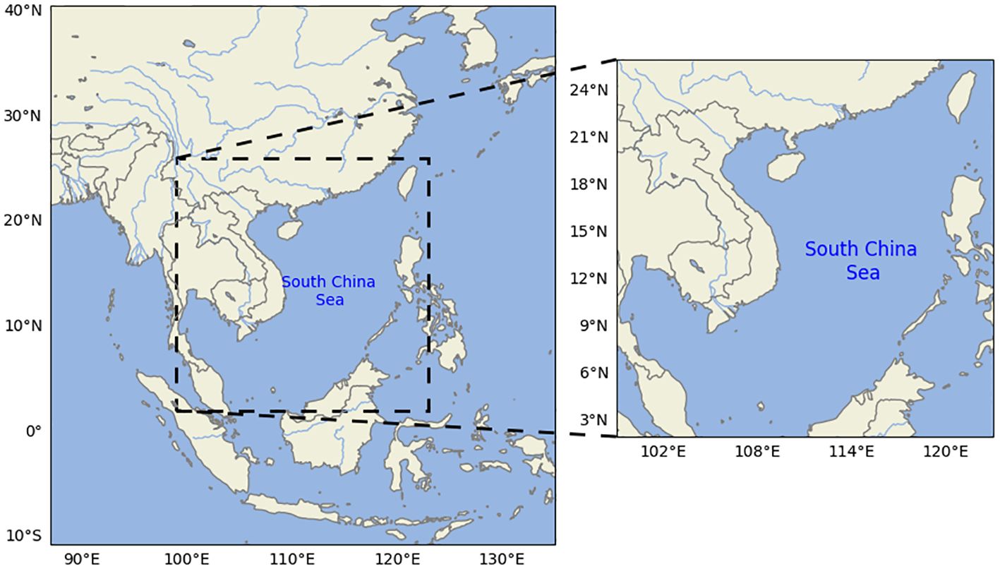
Figure 1 The study area of this paper. It is the South China Sea, specifically located between 2°N-26°N latitude and 99°E-123°E longitude.

2.2 Data

This study utilizes 10m u-wind component(u10), 10m v-wind component(v10), and SWH data from the ERA5 reanalysis dataset. ERA5, produced by the European Centre for Medium-Range Weather Forecasts (ECMWF), represents the fifth generation of atmospheric reanalysis and covers the period from 1950 to the present (Bell et al., 2021). The time range of the three datasets used in this study is from January 1, 2020, to December 31, 2021, with a temporal resolution of 1 hour, totaling 17,544 hours. The spatial resolution varies: the SWH data has a spatial resolution of 0.5° × 0.5°, while the u10 and v10 data have a spatial resolution of 0.25° × 0.25°. Table 1 shows information about the data. These data can be downloaded here (https://cds.climate.copernicus.eu/).

Table 1

Table 1 Data information.This study utilizes 10m U-wind component(U10), 10m V-wind component(V10), and SWH data from the ERA5 reanalysis dataset.

3 Materials and methods

This section presents the methodology used in this paper, the comparative models, and the evaluation metrics.

3.1 Soft attention mechanism

Attentional mechanisms serve as a technique for artificial neural networks to emulate human cognitive attention. By introducing weighted connections, these mechanisms enable the model to focus on crucial aspects of the input data selectively. In order to improve the precision of predictions, this study utilizes a soft attention mechanism. It assists the model in extracting relevant spatiotemporal information from the hidden states. By dynamically weighting the importance of different parts of the input sequence, this attention mechanism facilitates the model’s focus on pertinent details, thereby improving its predictive capabilities.

Figure 2A shows the structure of attention mechanism. It has two inputs: the hidden state of the previous moment and the input data of the current moment. They are summed up after a 2D convolutional layer, then passed through a tanh activation function and 2D convolution to get the attention score, which is then inputted into a softmax function to get the final attention weights. The above process can be represented by Equation 1.

Figure 2

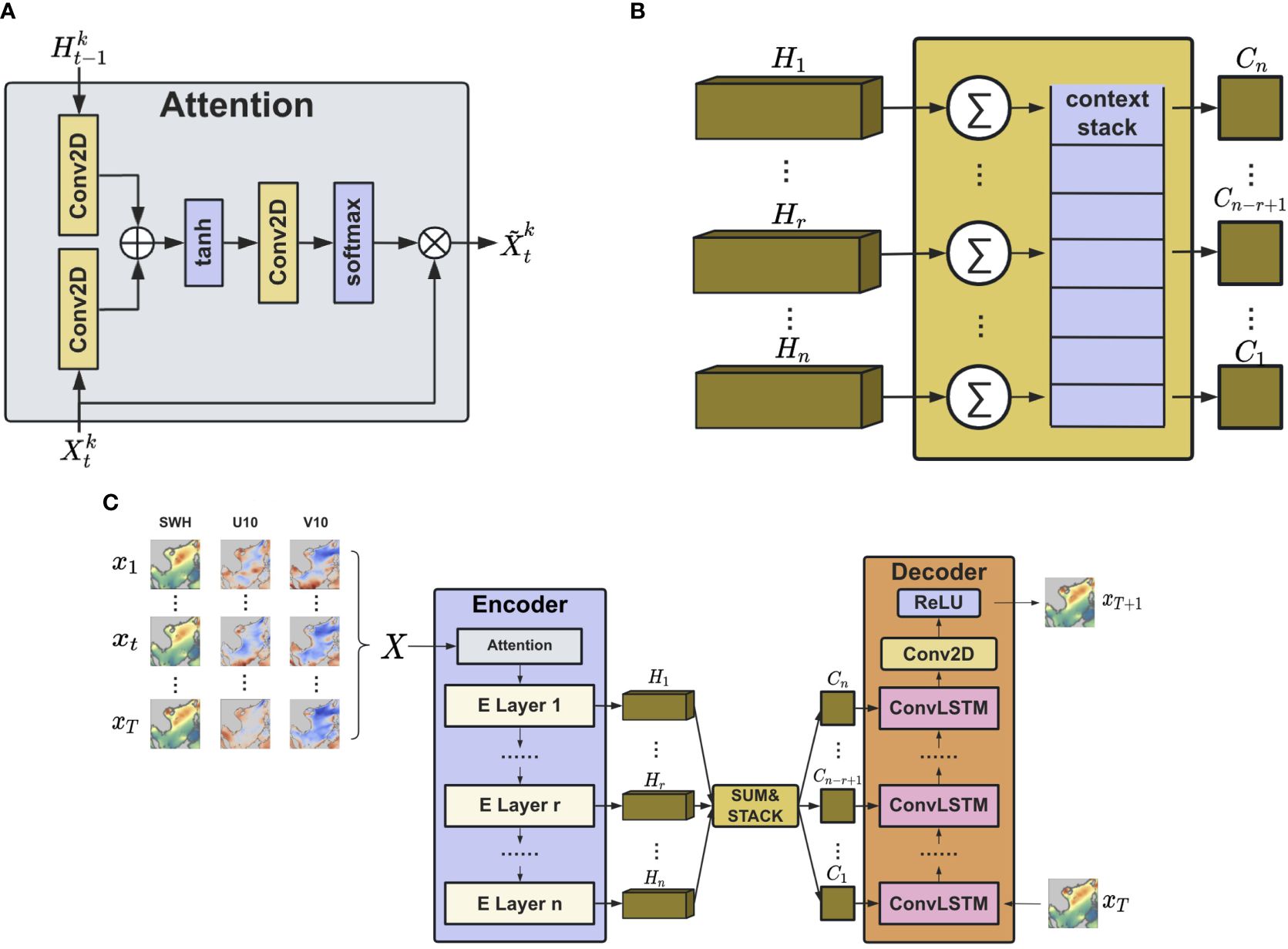
Figure 2 (A) The attention mechanism helps the model extract relevant spatiotemporal information from hidden states by dynamically weighting different parts of the input sequence, thereby improving its predictive capabilities. (B) The introduction of context vector can prevent the loss of valuable information when predicting long-term information. we define a context stack to store these vectors. (C) SAC-ConvLSTM combines the attention mechanism, context vector, and the ConvLSTM model for regional SWH prediction. Its overall structure is an encoder-decoder structure.

$\begin{array}{ll}\begin{array}{c}{A}_t^k=softmax(W*f (W_H*H_{t-1}^k+W_X*X_t^k))\\ {\tilde{X}}_t^k=A_t^k\circ X_t^k\end{array}& (1)\end{array}$

Here, $X_t^k$ is the current input of the kth channel, $H_t^k$ is the previous hidden state of the kth channel, f is the activation function, $W,W_H,W_X$ are all the trainable weight parameters. “°” denotes the Hadamard product. “∗” denotes the convolution operation.

3.2 Context vector

In order to prevent the loss of valuable information when predicting long-term information, this study introduces context vectors and defines a context stack to store these vectors. As shown in Figure 2B, We sum the hidden states of each encoder layer to obtain a context vector and then feed it into the context stack. The context vector of the first layer will be at the bottom of the stack, and subsequent context vectors will be stacked upwards. During the encoding phase, the encoder retrieves vectors from the context stack in sequence and combines them with input data for prediction. The process can be expressed by Equation 2.

$\begin{array}{ll}{C}_{n-r+1}={\displaystyle \sum _{j=1}^m{h}_r^j}& (2)\end{array}$

Here $C_{n-r+1}$ is the context vector for the (n-r+1)th layer of the decoder. $h_r^j$ denotes the jth hidden state of the rth layer of the encoder. m denotes the length of the input sequence.

3.3 Convolutional long and short-term memory

The spatiotemporal relationship between the data is essential in predicting Significant wave height. To effectively capture the spatiotemporal attributes inherent in sequential data, the Convolutional Long Short-Term Memory (ConvLSTM) algorithm draws on the powerful capabilities of Convolutional Neural Networks (CNNs) and Long Short-Term Memory Networks (LSTMs) (Shi et al., 2015). This research employs the ConvLSTM algorithm to forecast SWH in the South China Sea accurately. Its structure of is shown in Figure 3. The formula is as in Equation 3.

Figure 3

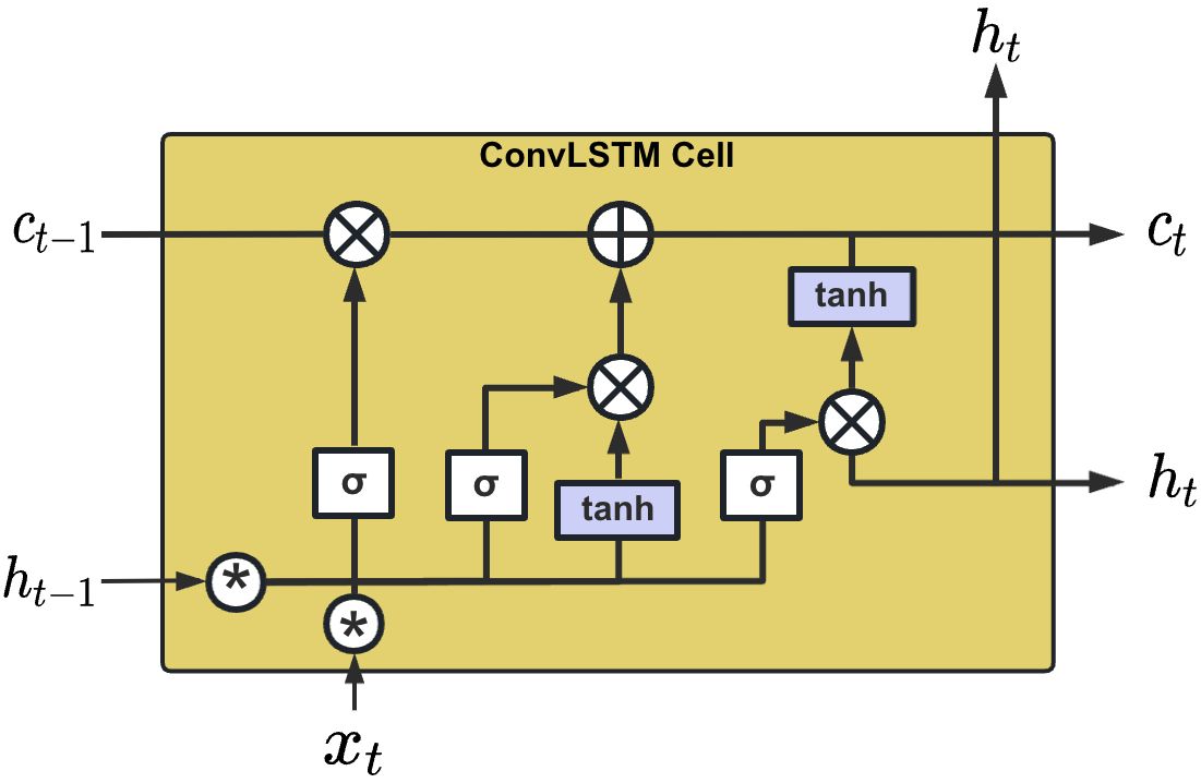
Figure 3 The structure of ConvLSTM. ConvLSTM combines the advantages of CNN and LSTM to effectively capture spatio-temporal dependencies in sequence data.

$\begin{array}{ll}\begin{array}{l}{i}_t=\sigma (W_{xi}\ast X_t+W_{hi}\ast H_{t-1}+W_{ci}\circ C_{t-1}+b_i)\\ {\tilde{X}}_t^k=A_t^k\circ X_t^k\\ f_t=\sigma (W_{xf}\ast X_t+W_{hf}\ast H_{t-1}+W_{cf}\circ C_{t-1}+b_f)\\ C_t=f_t\circ C_{t-1}+i_t\circ \tanh (W_{xc}\ast X_t+W_{hc}\ast H_{t-1}+b_c)\\ o_t=\sigma (W_{xo}\ast X_t+W_{ho}\ast H_{t-1}+W_{co}\circ C_{t-1}+b_o)\\ H_t=O_t\circ \tanh (C_t)\end{array}& (3)\end{array}$

Here $i_t,f_t$ and $o_t$ are the input gate, forget gate and output gate, respectively. X, C and H represent the input, cell state and hidden state, respectively. t and t −1 are current and previous time. W is the learnable weight parameters. b denotes the bias.“σ” represents the sigmoid function.

3.4 SAC-ConvLSTM

Combining the aforementioned attention mechanism, context vector, and ConvLSTM model, this study proposes a model for forecasting effective wave heights in ocean regions, named SAC-ConvLSTM. Its structure is illustrated in Figure 2C.

The model structure mainly consists of an encoder and a decoder. To ensure that the model captures the key features of the input sequence, we apply the soft attention mechanism before the encoder. The encoder primarily encodes the sequence processed through attention, capturing relevant information contained in the sequence. After each layer produces a result, it is transformed into a context vector, which is then added to the context stack. The decoder later retrieves these context vectors and combines them with input data to produce the output.

3.5 Comparative model

In this section, we present the comparative models used in this study: Simple Moving Average (SMA), Long and Short-Term Memory Network (LSTM), Trajectory Gated Recurrent Unit (TrajGRU) and Convolutional Gated Recurrent Unit (ConvGRU).

3.5.1 Simple Moving Average

SMA is a statistical method that looks at long-term trends by smoothing out time-series data. SMA can be used to predict SWH in the ocean. Its formula is shown in Equation 4 (Hansun, 2013).

$\begin{array}{ll}SM{A}_t=\frac{X_{t-1}+X_{t-2}+\dots +X_{t-\mathit{\text{(n}}+\mathrm{1)}}}{n}& (4)\end{array}$

Here $SM{A}_t$ represents the Simple Moving Average at time t, $X_t-i$ is the ocean significant wave height data at time t − i,n is the total length of the input sequence.

3.5.2 Long and Short-Term Memory Network

LSTM architecture significantly improves recurrent neural networks as it tackles the long-term dependency challenge. It accomplishes this through a gating mechanism comprising input, forget, and output gates, along with cell states. These gates regulate the flow of information and forgetting in a highly effective manner. The input gate determines the amount of current input data to retain in the cell state. The forget gate decides how much of the cell state from the previous moment should be preserved. Lastly, the output gate decides how much of the current cell state should be output to the output value. The model is defined as shown in Equation 5 (Hochreiter and Schmidhuber, 1997).

$\begin{array}{ll}\begin{array}{l}{i}_t=\sigma (W_{xi}{X}_t+W_{hi}{H}_{t-1}+b_i)\\ f_t=\sigma (W_{xf}{X}_t+W_{hf}{H}_{t-1}+b_f)\\ o_t=\sigma (W_{xo}{X}_t+W_{ho}{H}_{t-1}+b_o)\\ {ɡ}_t=\tanh (W_{xg}{X}_t+W_{hg}{H}_{t-1}+b_g)\\ C_t=f_t\circ C_{t-1}+i_t\circ g_t\\ h_t=o_t\circ \tanh (C_t)\end{array}& (5)\end{array}$

3.5.3 Convolutional Gated Recurrent Unit

Similar to ConvLSTM, ConvGRU replaces the LSTM units with GRU units. GRU, which stands for Gated Recurrent Unit, can be viewed as a variant of LSTM. It optimizes the cell structure of LSTM neural networks, reducing parameters and accelerating training. GRU simplifies the LSTM architecture by combining the input and forget gates into a single update gate while discarding the memory unit. Whenever there is an input to the ConvGRU, the reset gate will decide whether to clear the previous state, and the update gate will choose how much information to write to the state. ConvGRU is calculated as in Equation 6 (Shi et al., 2017).

$\begin{array}{ll}\begin{array}{c}{Z}_t=\sigma (W_z*X_t+U_z*H_{t-1}+b_z)\\ R_t=\sigma (W_r*X_t+U_r*H_{t-1}+b_r)\\ H_t^{\text{'}}=f(W_h*X_t+R_t\circ (U*H_{t-1})+b_h)\\ H_t=(1-Z_t)\circ H_t^{\text{'}}+Z_t\circ H_{t-1}\end{array}& (6)\end{array}$

Here $Z_t$ and $R_t$ denote the update and reset gate. X and H represent the input and hidden state, respectively. W and U denote the weights and bias. f is the activation function.“°” is the Hadamard product. “σ” is the sigmoid function.

3.5.4 Trajectory Gated Recurrent Unit

The Trajectory Gated Recurrent Unit (TrajGRU) generates the local neighborhood set for each location using the current input and previous state at each timestamp (Shi et al., 2017). It has dynamically determined recurrent connections. TrajGRU improves on the convolution operation in ConvGRU. The convolution operation basically applies a location-invariant filter to the input. i.e., the connection structure and weights are fixed for all the locations. The main formulas of TrajGRU are given as Equation 7.

$\begin{array}{ll}\begin{array}{c}\begin{array}{c}{U}_t,V_t=\gamma (X_t,H_{t-1})\\ Z_t=\sigma \left(W_{xz}\ast X_t+{\displaystyle \sum _{l=1}^L{W}_{hz}^l\ast warp(H_{t-1},U_{t,l},V_{t,l})+b_z}\right)\end{array}\\ R_t=\sigma \left(W_{xr}\ast X_t+{\displaystyle \sum _{l=1}^L{W}_{hr}^l\ast warp(H_{t-1},U_{t,l},V_{t,l})+b}\right)\\ H_t^{\text{'}}=f\left(W_{xh}\ast X_t+R_t\circ \left({\displaystyle \sum _{l=1}^L{W}_{hh}^l\ast warp(H_{t-1},U_{t,l},V_{t,l})}\right)+b_h\right)\\ H_t=(1-Z_t)\circ H_t^{\text{'}}+Z_t\circ H_{t-1}\end{array}& (7)\end{array}$

Where $X_t$ is the input. $Z_t$ and $R_t$ denote the update and reset gate, respectively., $H_t$ and $H_t^{\text{'}}$ are the memory state and new information. $U_t,V_t$ represent the flow fields that store the local connection structure generated by the structure generating network γ. The $warp$ mainly implements local variation so that neighboring points can be randomly selected to capture the motion of the image.

3.6 Evaluation metrics

In this study, we will use mean absolute error (MAE), root mean square error (RMSE), mean square error (MSE), and Pearson correlation coefficient (PCC) to quantitatively assess the predictive effectiveness of the models. They are calculated as expressed in Equations 8–11.

$\begin{array}{ll}MAE=\frac{1}{n}{\displaystyle \sum _{i=1}^n\left|y_{truth}-y_{pred}\right|}& (8)\end{array}$

$\begin{array}{ll}MSE=\frac{1}{n}{\displaystyle \sum _{i=1}^n{(y_{truth}-y_{pred})}^2}& (9)\end{array}$

$\begin{array}{ll}RMSE=\sqrt{MSE}=\sqrt{\frac{1}{n}{{\displaystyle \sum _{i=1}^n(y_{truth}-y_{pred})}}^2}& (10)\end{array}$

$\begin{array}{ll}PCC=\frac{{\displaystyle {\sum }_{i=1}^n(y_{pre{d}_i}-{\overline{y}}_{pred})}(y_{trut{h}_i}-{\overline{y}}_{truth})}{\sqrt{{\displaystyle {\sum }_{i=1}^n{(y_{pre{d}_i}-{\overline{y}}_{pred})}^2}{\displaystyle {\sum }_{i=1}^n{(y_{trut{h}_i}-{\overline{y}}_{truth})}^2}}}& (11)\end{array}$

Where n denotes the total number of predicted SWH, $y_{true}$ is the true value, $y_{pred}$ is the predicted value, ${\overline{y}}_{truth}$ is the mean of the true values, ${\overline{y}}_{pred}$ is the mean of the predicted values.

4 Experiments and results analysis

The software environment for the experiments in this study includes Ubuntu 18.04, Python 3.8, Pytorch 2.1.2, Matplotlib 3.4.2, and NumPy 1.21.1. The hardware environment comprises an i9–13900K processor, 64 GB of RAM, and an NVIDIA GTX 4080 graphics card. We employ an early-stopping mechanism during training with a patience value of 20. The initial learning rate is set to 0.001, and the learning rate is adjusted using ReduceLROnPlateau, with a patience value of 4. The specific experimental parameters are configured as follows in Table 2.

Table 2

Table 2 Parameter setting.

4.1 Input sequence length

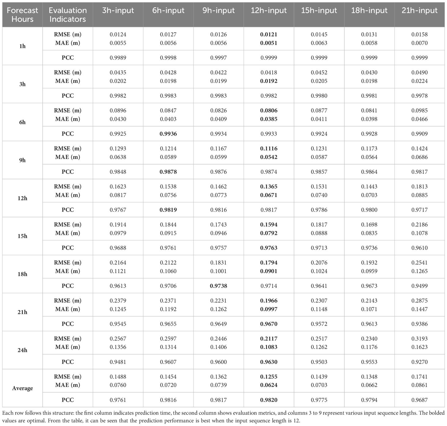
One of the characteristics of spatiotemporal sequence prediction is its ability to capture the spatiotemporal relationship within sequence data. Therefore, the length of the input sequence significantly influences prediction accuracy. This study conducted experiments on the input sequence length of the model to get the best prediction results. Table 3 shows the MAE, RMSE, PCC, and average values predicted by the model for different input sequence lengths. The first row represents the input length, the first column represents the prediction time, and the second represents the evaluation metrics. The bolded values are optimal. From the table, it can be observed that as the sequence length increases, the predictive performance does not necessarily improve. This could be because excessively short input sequences fail to provide sufficient information for the model to capture the features in the data. Conversely, overly long input sequences may contain much redundant information, leading to a decrease in model prediction accuracy. Overall, the best predictive performance is observed when the input sequence length is 12, while it is poorest when the length is 21. Therefore, the input length for the model in this study will be set to 12.

Table 3

Table 3 The evaluation metrics for SWH prediction with different input sequence lengths.

4.2 Model comparison

Figure 4 depicts the evaluation metrics of each model for SWH forecasts for the next 1–24 hours. As can be seen from the four plots, the RMSE, MAE, MSE, and PCC predicted by all models except the LSTM model are close to each other in the first 6 hours of SWH. As the prediction time increases, each model’s RMSE, MAE, and MSE gradually increase, and the PCC decreases. At the same time, the prediction gap of each model starts to increase with prediction as well, especially after 12 hours. Compared to the other models, the SAC-ConvLSTM model has a smoother curve, indicating that the model has the best prediction performance.

Figure 4

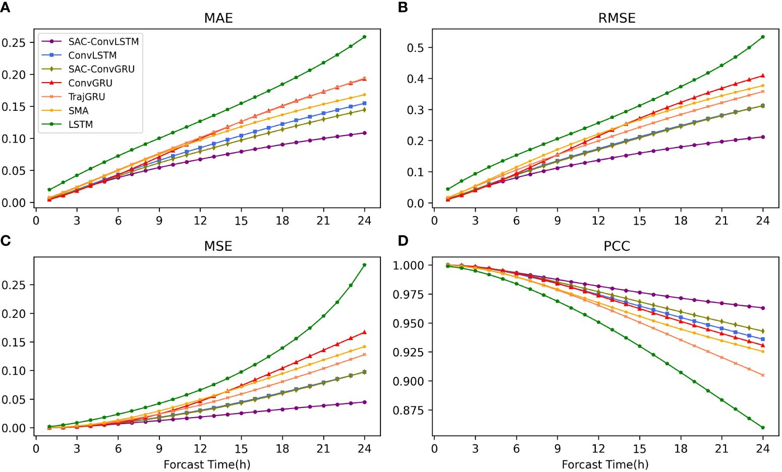
Figure 4 The evaluation metrics of each model for SWH prediction for the next 1-24 hours. (A–D) represent MAE, RMSE, MSE, and PCC, respectively. It can be seen that the prediction performance of the models decreases as the prediction time grows, but the SAC-ConvLSTM model has a smoother decreasing trend compared to the other models. This also indicates that it has the best prediction performance.

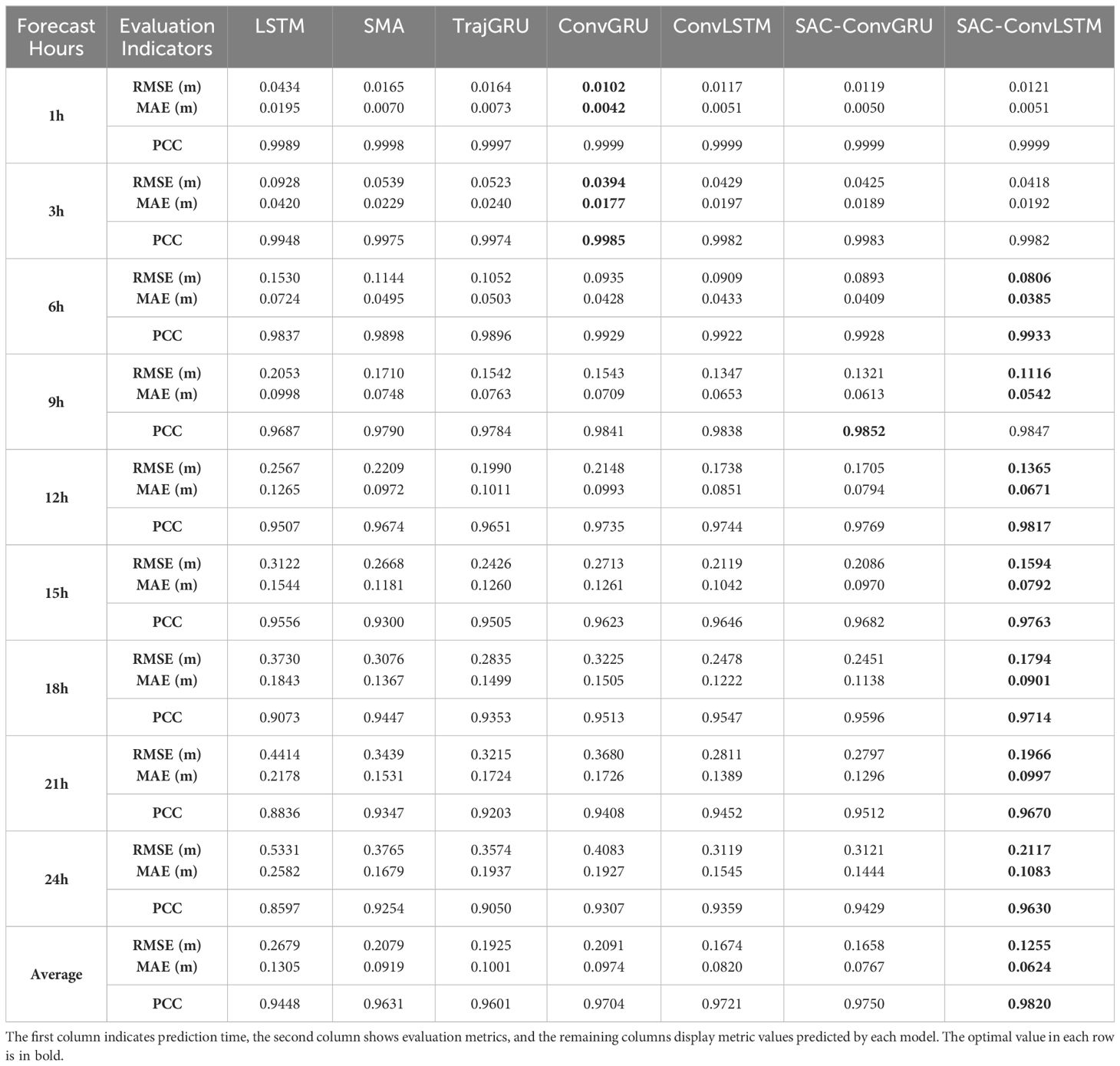
Table 4 shows the RMSE, MAE, and PCC, as well as the mean values of each model for predicting SWH for the next 1–24 hours. The table shows that the SAC-ConvLSTM model is better than the other models for most of the prediction time. In predicting the 24-h SWH, its RMSE, MAE, and PCC were 0.2117m, 0.1083m, and 0.9630, respectively. Compared with other models, the RMSE of SAC-ConvLSTM’s 24-hour average SWH prediction was reduced by 24% 53%, and the MAE was reduced by 18% 52%. Combining the prediction results of SAC-ConvLSTM with ConvLSTM and SAC-ConvGRU with ConvGRU, SA, and Context vector can significantly improve the prediction accuracy of SWH prediction. Compared with no SAC, its 24-hour average RMSE decreased by 25% and 26%, MAE decreased by 24% and 21%, and PCC improved by 1.02% and 0.47%, respectively. In summary, SAC-ConvLSTM has the optimal performance for 24-hour SWH prediction among all the models.

Table 4

Table 4 The evaluation metrics for SWH prediction by different models.

To compare the SWH prediction performance of each model more intuitively, we visualized the prediction results. Figure 5 shows the prediction plots of each model for 1, 3, 6, 9, 12, 15, 18, 21, and 24 hours, respectively. The first row represents the ground truth (ERA5 data), while the subsequent rows display the prediction plots of each model. We observe that the prediction results of each model exhibit minimal differences in the prediction plots of 1, 3, and 6 hours. However, as the prediction horizon increases, especially in the 15–24 hour range, disparities in the prediction results of each model become more apparent. In particular, the SAC-ConvLSTM model performs better in predicting the region with high values in the lower left part of the South China Sea. In contrast, other models demonstrate poorer prediction in this area. This suggests that the proposed model performs well in 24-hour SWH prediction and exhibits strong performance overall.

Figure 5

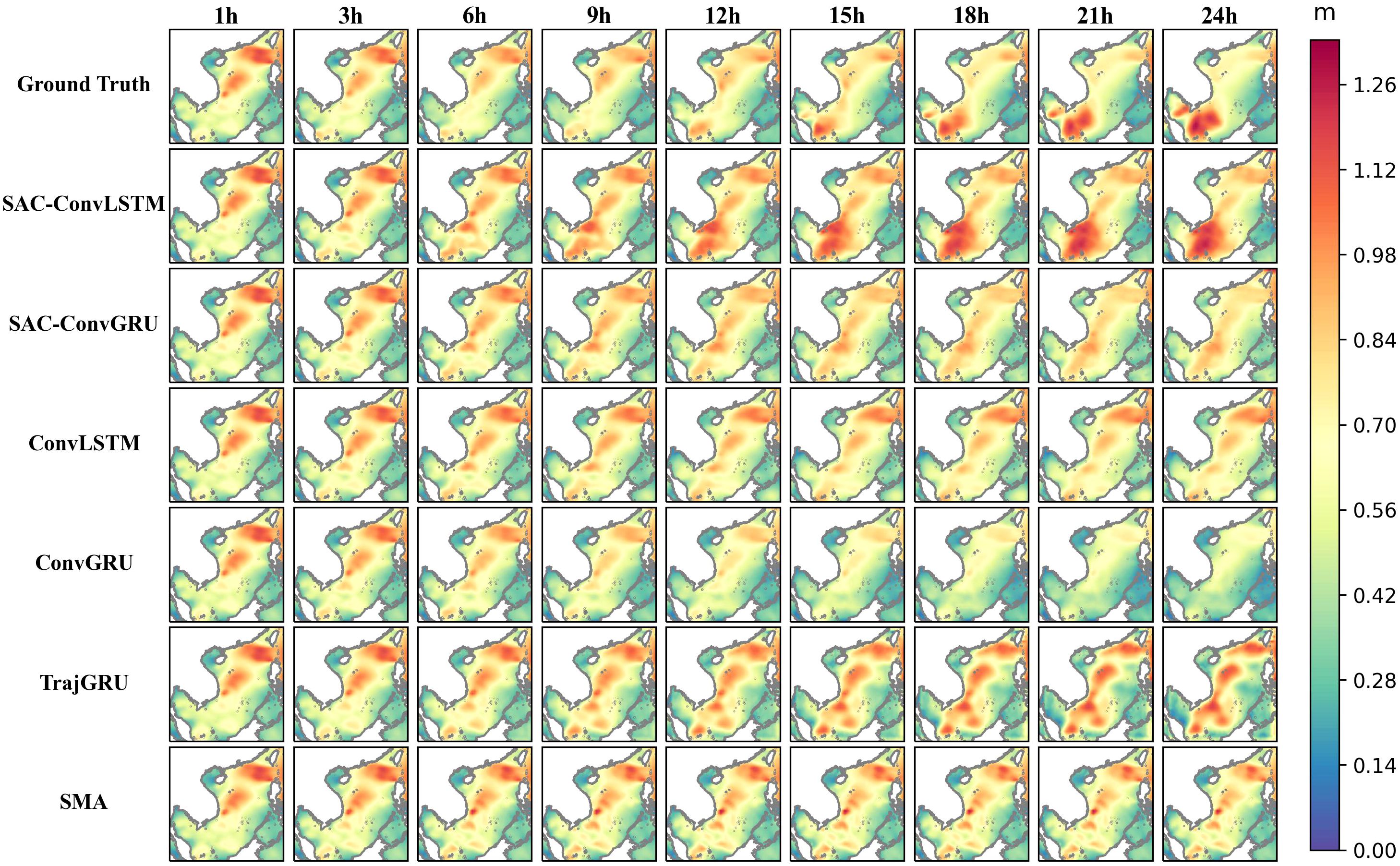
Figure 5 The prediction results of all models for SWH. The first row is the ground truth (ERA5 data). Other rows are the various methods. Each row of 9 images represents the prediction results for 1-24 hours.

4.3 The effect of wind on wave prediction

A close connection exists between sea surface winds and waves in physical oceanography. Generally, the effective wave height is positively correlated with the magnitude of the sea surface winds. In other words, higher sea surface winds result in more giant waves, whereas lower sea surface winds lead to smaller waves. This correlation underscores the influence of wind on wave dynamics and highlights the interdependence of these two oceanic phenomena. Therefore, in order to investigate the effect of sea surface winds on the prediction of significant wave height in the ocean, we set up four scenarios using two models, SAC-ConvLSTM and ConvLSTM, respectively, to carry out the experiments, and their specific settings are shown in Table 5.

Table 5

Table 5 The information of four scenarios.

To better illustrate the impact of wind on SWH prediction, we present comparisons for different models separately. Figure 6 illustrates the results of this experiment. When wind is included as an input, it improves wave prediction when both models are used. As the forecast time increases, the MAE and RMSE with the wind as input compared to single significant wave height (SWH) input have improved by over 20% at 24 hours.

Figure 6

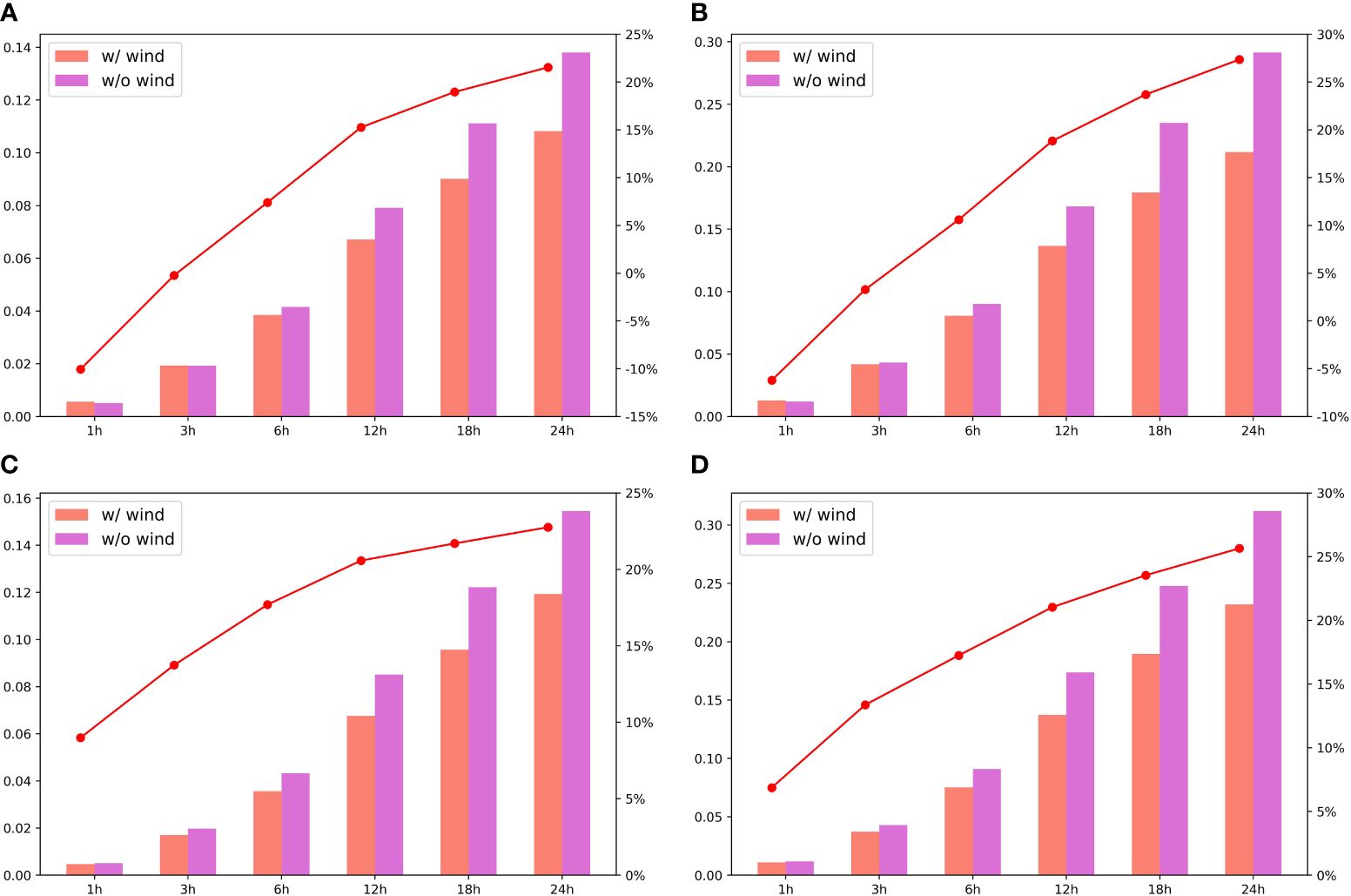
Figure 6 The experimental results on the effect of wind on SWH prediction, (A, B) are the MAE, RMSE, and lift percentages for Scenarios 1 and 2, while (C, D) are for Scenarios 3 and 4. The bar charts show the values and the line charts show the percentage lift.

Figure 7 shows the ground truth and the predictions for the four scenarios. The first row represents the ground truth (ERA5 data), while the remaining four rows represent predictions for each scenario. It can be observed that Scenario 2 and 4 with a single SWH as input do not forecast the high-value region well. As the prediction time increases, its prediction becomes worse. However, after adding wind to the inputs, Scenario 1 and Scenario 3 improved their predictions relative to Scenario 2 and Scenario 4. In particular, Scenario 1, the SAC-ConvLSTM model, with the wind as an input, has been successful in its ability to capture and predict changes in the high-value region.

Figure 7

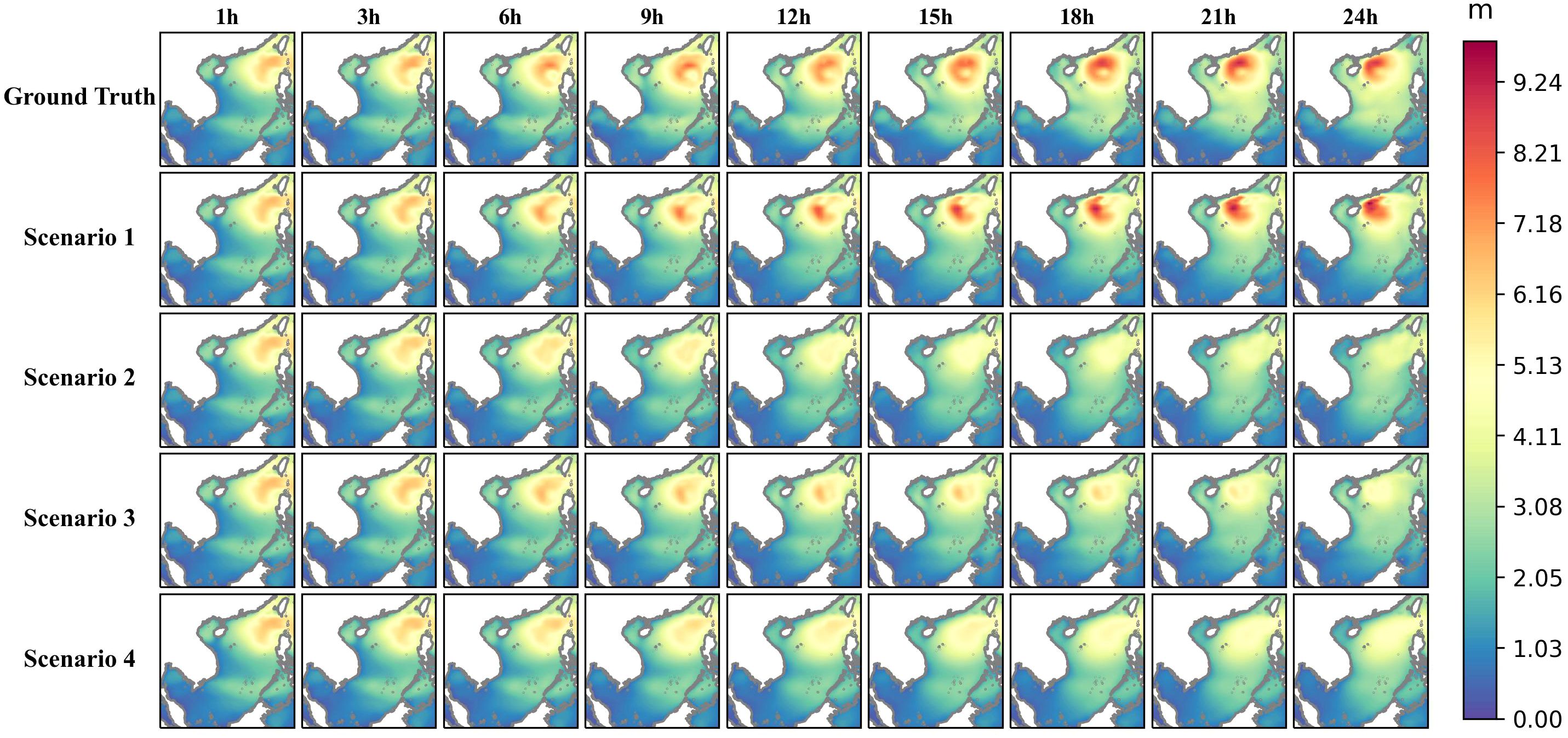
Figure 7 The comparison of 24-hour SWH prediction results under each scenario. The first row represents the ground truth (ERA5 data). Other rows represent the predicted results for each scenario.

4.4 Extreme weather

Due to the monsoon and climatic factors, the South China Sea frequently experiences extreme weather conditions. To evaluate the prediction performance of our model under such conditions, we selected seven instances of extreme weather for experimentation. Table 6 presents the information related to extreme weather events.

Table 6

Table 6 The information on extreme weather events.

Figures 8A-G shows the average of the 24-hour predictions of the present model with ConvLSTM and their errors during seven extreme weather periods. In each graph, the top row displays, from left to right, the ground truth, the present model’s predicted value, and the ConvLSTM model’s predicted value, respectively. Meanwhile, the first graph in the second row illustrates the error between the predicted value and the ground truth of the present model, and the second graph represents the error between the predicted value and the ground truth of the ConvLSTM model. In most cases, the present model outperforms the ConvLSTM model for 24-hour prediction under extreme weather conditions. This advantage is especially significant in nearshore areas. For example, in the coastal area in the northern part of the South China Sea, the prediction result of the ConvLSTM model is on the high side, while in the coastal area in the southern part of the South China Sea, its prediction result is on the low side. In contrast, this is hardly the case for the SAC-ConvLSTM model. It is evident that, in most cases, the 24-hour prediction performance of the present model outperforms that of the ConvLSTM model under extreme weather conditions. This difference is particularly pronounced in the nearshore areas, where the ConvLSTM model tends to overpredict in the northern nearshore region of the South China Sea and underpredict in the southern nearshore region. Conversely, such discrepancies are scarcely observed in the present model’s predictions.

Figure 8

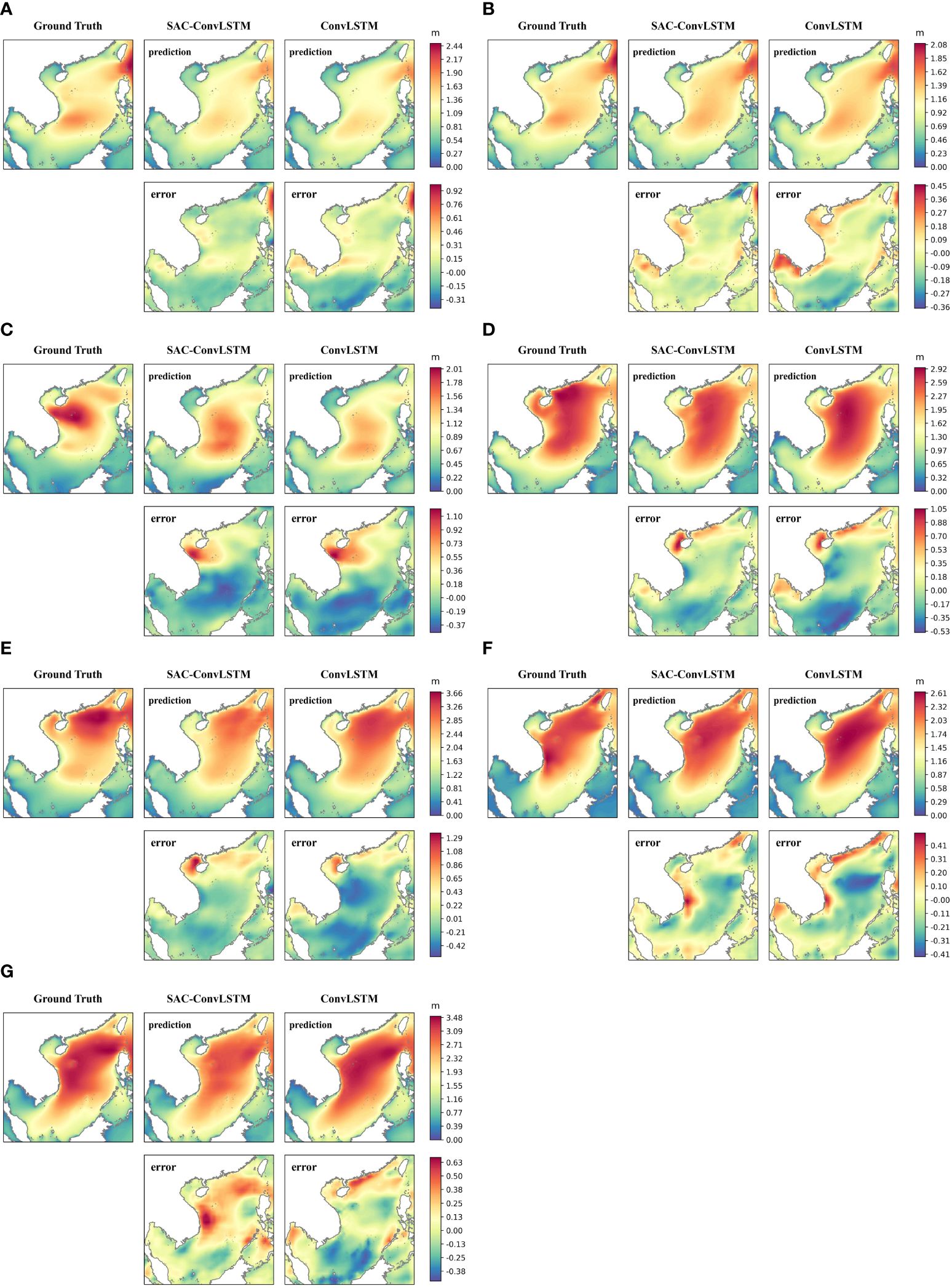
Figure 8 The averages of the 24-hour SWH predictions of the present model with ConvLSTM and their errors during seven extreme weather periods. (A–G) are Conson, Chanthu, Dianmu, Lionrock, Kompasu, the tropical depression, and Rai in sequence. Each subplot shows: first row (left to right) - ground truth (ERA5), SAC-ConvLSTM prediction, ConvLSTM prediction; second row - SAC-ConvLSTM error, ConvLSTM error.

5 Discussion and conclusion

This paper proposes a deep learning model named SAC-ConvLSTM to perform 24-hour prediction with the significant wave height in the South China Sea. Moreover, 17,544 hours of ERA5 reanalysis data from January 1, 2020, to December 31, 2021, are used to train, validate, and test the model. MAE, RMSE, MSE, and PCC are used to quantify the model’s predictive performance. 12 is chosen as the length of the input sequence. The results show that the SAC-ConvLSTM model has the best prediction performance compared to SMA, LSTM, TrajGRU, ConvGRU, and SAC-ConvGRU, with RMSE, MAE, and PCC of 0.2117m, 0.1083m, and 0.9630 at 24-hour prediction, respectively. This paper also investigates the effect of wind on wave prediction, and the results show that the longer the prediction time, the more the wind improves the accuracy of wave prediction, with the RMSE and MAE improving by more than 20% at 24 hours. The SAC-ConvLSTM model also has good prediction performance compared to the ConvLSTM model during extreme weather, especially in coastal areas.

However, in this paper, only wind and SWH are used as inputs, so other physical variables related to wave prediction, such as mean wave period and sea surface air pressure, can also be considered inputs to train the model in future studies. The study area of this paper is limited to the South China Sea, but it can be extended to other sea areas such as the Bohai Sea, Yellow Sea, and East China Sea in the future.

Data availability statement

Publicly available datasets were analyzed in this study. This data can be found here: https://cds.climate.copernicus.eu/.

Author contributions

BH: Software, Writing – original draft, Writing – review & editing, Data curation, Investigation, Visualization. HF: Investigation, Software, Visualization, Writing – original draft, Writing – review & editing, Conceptualization, Formal analysis, Methodology. XL: Funding acquisition, Investigation, Resources, Validation, Visualization, Writing – original draft. TS: Formal analysis, Methodology, Project administration, Supervision, Validation, Writing – review & editing, Conceptualization, Funding acquisition, Resources, Software. ZZ: Data curation, Methodology, Project administration, Supervision, Validation, Writing – review & editing.

Funding

The author(s) declare financial support was received for the research, authorship, and/or publication of this article. This work was jointly supported by the Major Projects of National Natural Science Foundation of China (U20A20105), National Key Research and Development Project of China (2021YFA1000103, 2021YFA1000102), National Natural Science Foundation of China (Grant Nos. 61972416, 62272479, 62202498), Taishan Scholarship (tsqn201812029), Shandong Provincial Natural Science Foundation(ZR2021QF023), Fundamental Research Funds for the Central Universities (21CX06018A), Spanish project PID2019-106960GB-I00, Juan de la Cierva IJC2018-038539-I.

Acknowledgments

In the process of researching and writing this paper, I would like to express my gratitude to everyone who has helped me. Additionally, I would like to extend my appreciation to the European Centre for Medium-Range Weather Forecasts for their contribution of the data sources utilized in this study.

Conflict of interest

The authors declare that the research was conducted in the absence of any commercial or financial relationships that could be construed as a potential conflict of interest.

Publisher’s note

All claims expressed in this article are solely those of the authors and do not necessarily represent those of their affiliated organizations, or those of the publisher, the editors and the reviewers. Any product that may be evaluated in this article, or claim that may be made by its manufacturer, is not guaranteed or endorsed by the publisher.

Footnotes

1. ^ Fusco, F. (2009). Short-term wave forecasting as a univariate time series problem.

References

Adnan R. M., Sadeghifar T., Alizamir M., Azad M. T., Makarynskyy O., Kisi O., et al. (2023). Short-term probabilistic prediction of significant wave height using bayesian model averaging: Case study of chabahar port, Iran. Ocean Eng. 272, 113887. doi: 10.1016/j.oceaneng.2023.113887

CrossRef Full Text | Google Scholar

Agrawal J., Deo M. (2002). On-line wave prediction. Mar. Structures 15, 57–74. doi: 10.1016/S0951-8339(01)00014-4

CrossRef Full Text | Google Scholar

Ali M., Prasad R., Xiang Y., Deo R. C. (2020). Near real-time significant wave height forecasting with hybridized multiple linear regression algorithms. Renewable Sustain. Energy Rev. 132, 110003. doi: 10.1016/j.rser.2020.110003

CrossRef Full Text | Google Scholar

Bell B., Hersbach H., Simmons A., Berrisford P., Dahlgren P., Horanyi,´ A., et al. (2021). The era5 global reanalysis: Preliminary extension to 1950. Q. J. R. Meteorological Soc. 147, 4186–4227. doi: 10.1002/qj.4174

CrossRef Full Text | Google Scholar

Booij N., Ris R. C., Holthuijsen L. H. (1999). A third-generation wave model for coastal regions: 1. model description and validation. J. Geophysical Research: Oceans 104, 7649–7666. doi: 10.1029/98JC02622

CrossRef Full Text | Google Scholar

Cao H., Liu G., Huo J., Gong X., Wang Y., Zhao Z., et al. (2023). Multi factors-predrnn based significant wave height prediction in the bohai, yellow, and east China seas. Front. Mar. Sci. 10, 1197145. doi: 10.3389/fmars.2023.1197145

CrossRef Full Text | Google Scholar

Deo M. C., Jha A., Chaphekar A., Ravikant K. (2001). Neural networks for wave forecasting. Ocean Eng. 28, 889–898. doi: 10.1016/S0029-8018(00)00027-5

CrossRef Full Text | Google Scholar

Ding J., Deng F., Liu Q., Wang J. (2023). Regional forecasting of significant wave height and mean wave period using eof-eemd-scinet hybrid model. Appl. Ocean Res. 136, 103582. doi: 10.1016/j.apor.2023.103582

CrossRef Full Text | Google Scholar

Feng Z., Hu P., Li S., Mo D. (2022). Prediction of significant wave height in offshore China based on the machine learning method. J. Mar. Sci. Eng. 10, 836. doi: 10.3390/jmse10060836

CrossRef Full Text | Google Scholar

Gao R., Li R., Hu M., Suganthan P. N., Yuen K. F. (2023). Dynamic ensemble deep echo state network for significant wave height forecasting. Appl. Energy 329, 120261. doi: 10.1016/j.apenergy.2022.120261

CrossRef Full Text | Google Scholar

Group, The Wamdi. (1988). The WAM model—A third generation ocean wave prediction model. Journal of Physical Oceanography. 18, 1775–1810.

Google Scholar

Gu C., Li H. (2022). Review on deep learning research and applications in wind and wave energy. Energies 15, 1510. doi: 10.3390/en15041510

CrossRef Full Text | Google Scholar

Guo M.-H., Xu T.-X., Liu J.-J., Liu Z.-N., Jiang P.-T., Mu T.-J., et al. (2022). Attention mechanisms in computer vision: A survey. Comput. Visual Media 8, 331–368. doi: 10.1007/s41095-022-0271-y

CrossRef Full Text | Google Scholar

Han L., Ji Q., Jia X., Liu Y., Han G., Lin X. (2022). Significant wave height prediction in the South China Sea based on the convlstm algorithm. J. Mar. Sci. Eng. 10, 1683. doi: 10.3390/jmse10111683

CrossRef Full Text | Google Scholar

Hansun S. (2013). “A new approach of moving average method in time series analysis”, 2013 conference on new media studies (CoNMedia).

Google Scholar

Hao P., Li S., Gao Y. (2023). Significant wave height prediction based on deep learning in the South China Sea. Front. Mar. Sci. 9, 1113788. doi: 10.3389/fmars.2022.1113788

CrossRef Full Text | Google Scholar

Hochreiter S., Schmidhuber J. (1997). Long Short-Term. Neural Computation 9(8), 1735–1780. doi: 10.1162/neco.1997.9.8.1735

PubMed Abstract | CrossRef Full Text | Google Scholar

Jain P., Deo M. (2006). Neural networks in ocean engineering. Ships offshore structures 1, 25–35. doi: 10.1533/saos.2004.0005

CrossRef Full Text | Google Scholar

Jain P., Deo M., Latha G., Rajendran V. (2011). Real time wave forecasting using wind time history and numerical model. Ocean Model. 36, 26–39. doi: 10.1016/j.ocemod.2010.07.006

CrossRef Full Text | Google Scholar

Juan N. P., Valdecantos V. N. (2022). Review of the application of artificial neural networks in ocean engineering. Ocean Eng. 259, 111947. doi: 10.1016/j.oceaneng.2022.111947

CrossRef Full Text | Google Scholar

Komen G. J., Cavaleri L., Donelan M., Hasselmann K., Hasselmann S., Janssen P. A. E. M. (1996). Dynamics and modelling of ocean waves.

Google Scholar

Lee H. S. (2015). Evaluation of WAVEWATCH III performance with wind input and dissipation source terms using wave buoy measurements for October 2006 along the east Korean coast in the East Sea. Ocean Engineering. (Elsevier) 100, 67–82.

Google Scholar

Liang B., Gao H., Shao Z. (2019). Characteristics of global waves based on the third-generation wave model swan. Mar. Structures 64, 35–53. doi: 10.1016/j.marstruc.2018.10.011

CrossRef Full Text | Google Scholar

Lionello P., Günther H., Janssen P. A. (1992). Assimilation of altimeter data in a global third-generation wave model. J. Geophysical Res.: Oceans 97, 14453–14474. doi: 10.1029/92JC01055

CrossRef Full Text | Google Scholar

Liu Y., Huang L., Ma X., Zhang L., Fan J., Jing Y. (2023). A fast, high-precision deep learning model for regional wave prediction. Ocean Eng. 288, 115949. doi: 10.1016/j.oceaneng.2023.115949

CrossRef Full Text | Google Scholar

Lou R., Lv Z., Dang S., Su T., Li X. (2023). Application of machine learning in ocean data. Multimedia Syst. 29, 1815–1824. doi: 10.1007/s00530-020-00733-x

CrossRef Full Text | Google Scholar

Luo Q.-R., Xu H., Bai L.-H. (2022). Prediction of significant wave height in hurricane area of the atlantic ocean using the bi-lstm with attention model. Ocean Eng. 266, 112747. doi: 10.1016/j.oceaneng.2022.112747

CrossRef Full Text | Google Scholar

Mahdavi-Meymand A., Sulisz W. (2023). Application of nested artificial neural network for the prediction of significant wave height. Renewable Energy 209, 157–168. doi: 10.1016/j.renene.2023.03.118

CrossRef Full Text | Google Scholar

Mahjoobi J., Mosabbeb E. A. (2009). Prediction of significant wave height using regressive support vector machines. Ocean Eng. 36, 339–347. doi: 10.1016/j.oceaneng.2009.01.001

CrossRef Full Text | Google Scholar

Malekmohamadi I., Bazargan-Lari M. R., Kerachian R., Nikoo M. R., Fallahnia M. (2011). Evaluating the efficacy of SVMs, BNs, ANNs and ANFIS in wave height prediction. Ocean Engineering. 38, 487–497.

Google Scholar

Meng F., Song T., Xu D., Xie P., Li Y. (2021). Forecasting tropical cyclones wave height using bidirectional gated recurrent unit. Ocean Eng. 234, 108795. doi: 10.1016/j.oceaneng.2021.108795

CrossRef Full Text | Google Scholar

Niu Z., Zhong G., Yu H. (2021). A review on the attention mechanism of deep learning. Neurocomputing 452, 48–62. doi: 10.1016/j.neucom.2021.03.091

CrossRef Full Text | Google Scholar

Pokhrel P., Ioup E., Hoque M. T., Simeonov J., Abdelguerfi M. (2020). Random forest classifier based prediction of rogue waves on deep oceans. arXiv preprint arXiv:2003.06431. doi: 10.48550/arXiv.2003.06431

CrossRef Full Text | Google Scholar

Reikard G., Rogers W. E. (2011). Forecasting ocean waves: Comparing a physics-based model with statistical models. Coast. Eng. 58, 409–416. doi: 10.1016/j.coastaleng.2010.12.001

CrossRef Full Text | Google Scholar

Ris R., Holthuijsen L., Booij N. (1999). A third-generation wave model for coastal regions: 2. verification. J. Geophysical Res.: Oceans 104, 7667–7681. doi: 10.1029/1998JC900123

CrossRef Full Text | Google Scholar

Shao W., Sheng Y., Li H., Shi J., Ji Q., Tan W., et al. (2018). Analysis of wave distribution simulated by wavewatch-iii model in typhoons passing beibu gulf, China. Atmosphere 9, 265. doi: 10.3390/atmos9070265

CrossRef Full Text | Google Scholar

Shi X., Chen Z., Wang H., Yeung D.-Y., Wong W.-K., Woo W.-c. (2015). Convolutional lstm network: A machine learning approach for precipitation nowcasting. Adv. Neural Inf. Process. Syst. 28.

Google Scholar

Shi X., Gao Z., Lausen L., Wang H., Yeung D.-Y., Wong W.-k., et al. (2017). Deep learning for precipitation nowcasting: A benchmark and a new model. Adv. Neural Inf. Process. Syst. 30.

Google Scholar

Shi W., Hu J. (2023). Spatiotemporal variation of anticyclonic eddies in the South China Sea during 1993–2019. Remote Sens. 15, 4720. doi: 10.3390/rs15194720

CrossRef Full Text | Google Scholar

Shi J., Su T., Li X., Wang F., Cui J., Liu Z., et al. (2023). A machine-learning approach based on attention mechanism for significant wave height forecasting. J. Mar. Sci. Eng. 11, 1821. doi: 10.3390/jmse11091821

CrossRef Full Text | Google Scholar

Soares C. G., Ferreira A., Cunha C. (1996). Linear models of the time series of significant wave height on the southwest coast of Portugal. Coast. Eng. 29, 149–167. doi: 10.1016/S0378-3839(96)00022-1

CrossRef Full Text | Google Scholar

Song T., Han R., Meng F., Wang J., Wei W., Peng S. (2022). A significant wave height prediction method based on deep learning combining the correlation between wind and wind waves. Front. Mar. Sci. 9, 983007. doi: 10.3389/fmars.2022.983007

CrossRef Full Text | Google Scholar

Song T., Pang C., Hou B., Xu G., Xue J., Sun H., et al. (2023a). A review of artificial intelligence in marine science. Front. Earth Sci. 11, 1090185. doi: 10.3389/feart.2023.1090185

CrossRef Full Text | Google Scholar

Song T., Wang J., Huo J., Wei W., Han R., Xu D., et al. (2023b). Prediction of significant wave height based on eemd and deep learning. Front. Mar. Sci. 10, 1089357. doi: 10.3389/fmars.2023.1089357

CrossRef Full Text | Google Scholar

Soydaner D. (2022). Attention mechanism in neural networks: where it comes and where it goes. Neural Computing Appl. 34, 13371–13385. doi: 10.1007/s00521-022-07366-3

CrossRef Full Text | Google Scholar

Tolman H. L. (2009). User manual and system documentation of WAVEWATCH III TM version 3.14. Technical note, MMAB contribution. 276.

Google Scholar

Umesh P. A., Behera M. R. (2021). On the improvements in nearshore wave height predictions using nested SWAN-SWASH modelling in the eastern coastal waters of India. Ocean Engineering. 236, 109550.

Google Scholar

VS, Enigo F. (2020). “Forecasting significant wave height using rnn-lstm models,” in 2020 4th International Conference on Intelligent Computing and Control Systems (ICICCS). 1141–1146 (IEEE).

Google Scholar

Wan W., Zhang J., Dai L., Liang H., Yang T., Liu B., et al. (2022a). A new snow depth data set over northern China derived using GNSS interferometric reflectometry from a continuously operating network (GSnow-CHINA v1.0, 2013–2022). 14 (8), 3549–3571. doi: 10.5194/essd-14-3549-2022

CrossRef Full Text | Google Scholar

Wan W., Zhao L., Zhang J., Liang H., Guo Z., Liu B., et al. (2022b). “Toward terrain effects on GNSS interferometric reflectometry snow depth retrievals: Geometries, modeling, and applications” in IEEE Transactions on Geoscience and Remote Sensing (IEEE).

Google Scholar

Wang H., Lei Z., Zhang X., Zhou B., Peng J. (2019). A review of deep learning for renewable energy forecasting. Energy Conversion Manage. 198, 111799. doi: 10.1016/j.enconman.2019.111799

CrossRef Full Text | Google Scholar

Wang Z., Li S., Dong S., Wu K., Yu H., Wang L., et al. (2018). Extreme wave climate variability in South China Sea. Int. J. Appl. Earth observation geoinformation 73, 586–594. doi: 10.1016/j.jag.2018.04.009

CrossRef Full Text | Google Scholar

Yang T., Wan W., Wang J., Liu B., Sun Z. (2022). A physics-based algorithm to couple CYGNSS surface reflectivity and SMAP brightness temperature estimates for accurate soil moisture retrieval. (IEEE) 60. doi: 10.1109/TGRS.2022.3156959

CrossRef Full Text | Google Scholar

Yang Y., Han L., Qiu C., Zhao Y. (2024). A short-term wave energy forecasting model using two-layer decomposition and lstm-attention. Ocean Eng. 299, 117279. doi: 10.1016/j.oceaneng.2024.117279

CrossRef Full Text | Google Scholar

Yevnin Y., Chorev S., Dukan I., Toledo Y. (2023). Short-term wave forecasts using gated recurrent unit model. Ocean Eng. 268, 113389. doi: 10.1016/j.oceaneng.2022.113389

CrossRef Full Text | Google Scholar

Yu S., Ma J. (2021). Deep learning for geophysics: Current and future trends. Rev. Geophysics 59, e2021RG000742. doi: 10.1029/2021RG000742

CrossRef Full Text | Google Scholar

Zhang X., Dai H. (2019). Significant wave height prediction with the crbm-dbn model. J. Atmospheric Oceanic Technol. 36, 333–351. doi: 10.1175/JTECH-D-18-0141.1

CrossRef Full Text | Google Scholar

Zhou S., Xie W., Lu Y., Wang Y., Zhou Y., Hui N., et al. (2021). Convlstm-based wave forecasts in the south and east China seas. Front. Mar. Sci. 8, 680079. doi: 10.3389/fmars.2021.680079

CrossRef Full Text | Google Scholar