Subantarctic pCO2 estimated from a biogeochemical float: comparison with moored observations reinforces the importance of spatial and temporal variability

Understanding the size and future changes of natural ocean carbon sinks is critical for the projection of atmospheric CO₂ levels. The magnitude of the Southern Ocean carbon flux has varied significantly over past decades but mechanisms behind this variability are still under debate. While high accuracy observations, e.g. from ships and moored platforms, are important to improve models they are limited through space and time. Observations from autonomous platforms with emerging biogeochemical capabilities, e.g. profiling floats, provide greater spatial and temporal coverage. However, the absolute accuracy of CO₂ partial pressure (pCO₂) derived from float pH sensors is not well constrained. Here we capitalize on data collected for over a year by a biogeochemical Argo float near the Southern Ocean Time Series observatory to evaluate the accuracy of pCO₂ estimates from floats beyond the initial in water comparisons at deployment. A latitudinal gradient of increasing pCO₂ southward and spatial variability contributed to observed discrepancies. Comparisons between float estimated pCO₂ and mooring observations were therefore restricted by temperature and potential density criteria (~ 7 µatm difference) and distance (1° latitude and longitude, ~ 11 µatm difference). By utilizing high quality moored and shipboard underway pCO₂ observations, and estimates from CTD casts, we therefore found that over a year, differences in pCO₂ between platforms were within tolerable uncertainties. Continued validation efforts, using measurements with known and sufficient accuracy, are vital in the continued assessment of float-based pCO₂ estimates, especially in a highly dynamic region such as the subantarctic zone of the Southern Ocean.

1 Introduction

With the unabated continuation of anthropogenic carbon emissions, understanding the magnitude and variability of natural carbon sinks is of critical importance for the projection of atmospheric CO₂ levels (Crisp et al., 2022). While the global oceans sequester approximately 25% of total CO₂ emissions every year (Sabine et al., 2004; Gruber et al., 2019; Friedlingstein et al., 2022), the Southern Ocean plays a disproportionately important role in this uptake, with some estimates as high as 50% over the past 125 years (Froehlicher et al., 2015; Le Quéré et al., 2018). In the Southern Ocean south of 35˚S, deep waters rich in dissolved inorganic carbon (DIC) and macronutrients upwell to the surface (Lumpkin and Speer, 2007; Marshall and Speer, 2012), stimulating both a natural release of CO₂ into the atmosphere through air-sea exchange, and an uptake of carbon through enhanced primary productivity (Gruber et al., 2009). The net magnitude of the carbon flux has varied significantly over the past decades (Landschützer et al., 2015; Lovenduski et al., 2015; Ritter et al., 2017; Keppler and Landschützer, 2019). Additionally, the strength in the different mechanisms driving this variability remains under debate, with each being influenced by a number of factors and external forcing, including changing wind patterns and upwelling intensities as well as changes in temperature, ocean circulation, and primary productivity (Gruber et al., 2019; McKinley et al., 2020; Wright et al., 2022).

High-quality carbon system observations are important to help improve models and track efforts to reduce anthropogenic carbon emissions. The highest quality CO₂ partial pressure (pCO₂) observations come from direct ship-based measurements that are calibrated in situ with CO₂ reference gases (≤ 0.5% µatm uncertainty). Similar methods are also used on Uncrewed Surface Vehicles (USVs), sailboats (Landschützer et al., 2023) and surface buoys (0.5% µatm uncertainty). Seawater pCO₂ calculated from discrete CTD water sample DIC and total alkalinity (TA) have slightly lower quality (~ 3% uncertainty). However, all aforementioned high-accuracy observations are limited in time and space, and are particularly scarce for the winter season in the Southern Ocean (Bakker et al., 2016). Observations from moored platforms can provide high accuracy data year-round but are limited spatially (Sutton et al., 2014a). Observations from autonomous platforms, such as USVs (Sabine et al., 2020; Sutton et al., 2021) or profiling floats (Gray et al., 2018; Sutton et al., 2021), provide greater spatial and temporal coverage. However, the accuracy of pCO₂ derived from pH sensors on biogeochemical (BGC) Argo floats, is not well constrained. The uncertainty assessment described in Williams et al. (2017) suggests a relative uncertainty in float-based pCO₂ of 2.7%, yet direct validation was limited to underway ship data taken at the time of float deployment. Assessments spanning the lifetime of a float are often made by comparing float-based pH data at depth to climatologies rather than continuous in-situ measurements over extended periods of time (Maurer et al., 2021). Comparisons between float based pCO₂ estimates and high accuracy observations beyond the time of deployment are limited by the rare overlap between float locations and shipboard or moored observations, such as floats passing by Time Series sites, e.g. the Drake Passage (Fay et al., 2018).

The Southern Ocean Time Series (SOTS), a part of Australia’s Integrated Marine Observing System (IMOS), provides high accuracy, direct pCO₂ observations from annually serviced Southern Ocean Flux Station (SOFS) moorings in the Indian sector of the subantarctic Zone (SAZ) southwest of Tasmania, (~47˚S, 142˚E, Figure 1). The SAZ is an important region of the Southern Ocean, where deep winter mixing to >400m (Rintoul and Trull, 2001) replenishes surface nutrients and, via the formation of Subantarctic Mode Water, supplies the subsurface southern hemisphere subtropical gyre with nutrients and oxygen (Sarmiento et al., 2004; Rintoul, 2006; Helm et al., 2011). This subduction of surface waters and the anthropogenic carbon they have sequestered, is a key process in the removal of anthropogenic carbon from the atmosphere for timescales that are meaningful in the context of human-induced climate change and mitigation (Langlais et al., 2017).

FIGURE 1

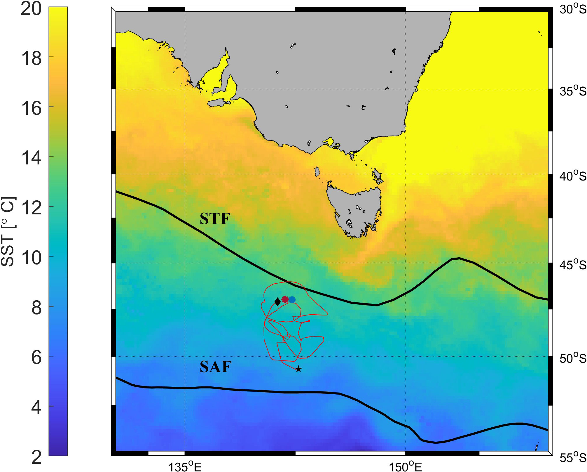
Figure 1 SOFS mooring (red * SOFS-9 deployed 31 August 2020, blue dot SOFS-10 deployed 20 April 2021) locations and BGC Argo float track (red line). The black diamond marks the deployment position of the float, the black star marks the last profile included in this study. Climatological mean frontal positions (Orsi et al., 1995) are indicated by the thick black lines, Subtropical Front (STF), Subantarctic Front (SAF). The background colormap shows SST (illustrated for January 2021) as estimated from satellite remote sensing (Ocean Productivity [oregonstate.edu)].

During the Southern Ocean Large Areal Carbon Export (SOLACE) voyage in 2020 (Ellwood et al., 2021) a BGC Argo float, equipped with a pH sensor (Sea-Bird Scientific SeaFET), was deployed within 40km of the SOTS site. For over a year this float drifted within an area between -46 to -51˚S and 140 to 145˚E (Figure 1), providing the unique opportunity to repeatedly compare high-accuracy in-situ mooring pCO₂ measurements with pCO₂ derived from float pH sensor data.

We will first compare float pH data and derived parameters such as TA and pCO₂ to other platforms, investigate sources of uncertainty and then discuss reasons for any disagreement between platforms.

2 Materials and methods

2.1 BGC Argo float data

BGC Argo float 5906623 was deployed in December 2020 during SOLACE voyage IN2020_V08 on the RV Investigator (https://mnf.csiro.au/en/Voyages/IN2020_V08). Due to the science objectives of this voyage the float was programmed with a non-standard sampling schedule at the start of its mission. This meant that for the first 5 months, deep cycles (to ~2000m) were interspersed with a set of shallow profiles (to 500m and 12h later to 1000m) every 2 days. This reduced the deep profile sampling frequency from the usual 10 days to between 11 and 15 days, with no deep profiles between 3 Feb 2021 and 4 March 2021.

A similar sampling schedule was re-instated in October 2021 to April 2022, with 12-hourly shallow profile sampling interspersed between deep profiles and only one deep profile between 21 October 2021 and 16 December 2021.

For float pCO₂ and air-sea flux calculations we used the delayed mode quality-controlled (QC) data (Argo variable PH_IN_SITU_ADJUSTED, pH_adj) as available from the Argo Global Data Assembly Center (GDAC). Delayed-mode quality control (DMQC) adjustment of float pH was performed at the Australian BGC Argo facility and followed Maurer et al. (2021) using reference estimates calculated from LIPHRv2 equation 7 at 1500m depth. Although there were discrete timeframes for which data at this depth was not available, using an alternate reference depth throughout these periods was not advised due to the greater uncertainty in reference estimates at shallower depth (Carter et al., 2018). Additionally, the longest period for which profiles did not reach QC depth was 32 days, with each period bounded on either side by deep profiles, providing anchors for DMQC assessment. Furthermore, erratic sensor drift during short time frames would be uncharacteristic of pH sensor behavior, so use of deep profiles at the frequency available was deemed sufficient in the DMQC process.

For float TA estimates (TA^PF, where ^PF stands for profiling float and is added to all float related parameters) we used the Locally Interpolated Alkalinity Regression (LIARv2) as described in Carter et al. (2018), which uses adjusted values of temperature, salinity (psal) and dissolved oxygen to estimate total alkalinity. Quality control of these parameters followed currently available best practice as outlined in Maurer et al. (2021). If pCO₂ is calculated from pH and TA, it differs from results based on DIC and TA samples and direct pCO₂ measurements. This is due to a difference between pH measured spectrophotometrically and pH calculated from DIC and TA (Carter et al., 2013; Williams et al., 2017). Therefore, before profiling float-based pCO₂ estimates (pCO₂^PF) can be compared to mooring observations, a bias correction was applied to each profile, as per Williams et al. (2017):

$\begin{array}{ll}p{H}^{adj corr} = p{H}_{adj} -\mathbf{0.034529} * p{H}_{1500m, 25˚C, 0dbar} + \mathbf{0.26709}& (1)\end{array}$

Where pH_{1500m, 25˚C, 0dbar} is the pH_adj at 1500m (the standard QC reference depth), adjusted to 25˚C and 0dbar. Note that application of this bias correction is in line with the current operational procedure for calculating pCO₂ from floats with SOCCOM and GO-BGC arrays (Riser et al., 2023).

The Matlab script CO2SYSv3.1.1 (Lewis and Wallace, 1998; van Heuven et al., 2011; Sharp et al., 2021) was used to calculate pCO₂^PF from float measured pH^{adj corr} and float estimated TA^PF, with dissociation constants of carbonate by Lueker et al. (2000), of fluoride from Perez and Fraga (1987), of sulphate from Dickson (1990) and the boron to salinity ratio by Lee et al. (2010). Silicate and phosphate concentration was taken from WOA18 annual averages as 2.5 µmol kg^-1 and 0.9 µmol kg^-1, respectively. NH₄ was set to 2 µmol kg^-1 and H₂S to 0 µmol kg^-1. Orr et al. (2018) found combined uncertainties in carbon system parameter estimates to be largely driven by uncertainties in dissociation constants. We therefore tried the most commonly used K₁ and K₂ constants by Lueker et al. (2000), as well as more recently refined constants by Schockman and Byrne (2021), which are experimentally determined with spectrophotometric methods and evaluated with shipboard and laboratory data.

For air-sea flux calculations (FCO₂^PF) we averaged the top 20m of each profile (Gray et al., 2018).

Air-sea fluxes were calculated as follows:

$\begin{array}{ll}FC{O}_2=k \alpha \Delta pC{O}_2& (2)\end{array}$

where k is the gas transfer velocity, scaled according to Fay et al. (2021) to account for the fact that we use ERA5 windspeeds, α is the coefficient of CO₂ solubility according to Weiss (1974) and ΔpCO₂ is the gradient between seawater pCO₂ and atmospheric pCO₂ such that negative FCO₂ indicates CO₂ uptake by the ocean and positive FCO₂ indicates outgassing.

Atmospheric pCO₂ data (pCO₂^PF_air) for the float location and profile times were calculated from mole fractions of CO₂ in dry air (xCO₂) from the CSIRO Oceans and Atmosphere and the Australian Bureau of Meteorology Kennaook/Cape Grim Baseline Air Pollution Station in Tasmania, Australia (https://capegrim.csiro.au/). The monthly data were interpolated on daily timesteps using piecewise cubic Hermite polynomials (Gray et al., 2018). Hourly windspeed and mean sea level pressure data from the ERA5 reanalysis product (0.25˚ gridded data, Hersbach et al., 2018) were subset to the nearest space coordinate of each float profile and interpolated on minute timesteps to the time of the float profile using piecewise cubic Hermite polynomials. Float seawater temperature and salinity together with ERA5 mean sea level pressure were used to calculate atmospheric pCO₂ from atmospheric xCO₂ following the method of Zeebe and Wolf-Gladrow (2001). For annual flux (FCO₂^PF) calculations, pCO₂^PF data were interpolated on daily timesteps using piecewise cubic Hermite polynomials (Gray et al., 2018) and then integrated for the calendar year 2021. Where more than one profile existed per day, the results were averaged for daily fluxes.

2.2 SOFS mooring sensor data and quality control

The SOFS mooring is recovered, and a new mooring deployed once a year from research voyages on RV Investigator, and mooring named sequentially (for more details refer to annual reports Wynn-Edwards et al., 2019; Wynn-Edwards et al., 2022). This study covers data from SOFS-9 (deployed 31 August 2020, recovered 25 April 2021) and SOFS-10 (deployed 20 April 2021, recovered 13 May 2022). Mooring seawater and atmospheric pCO₂ (from here on called pCO₂^M and pCO₂^M_air, respectively, where ^M stands for mooring and is added to all mooring related parameters) were measured by a Moored Autonomous pCO₂ System (MAPCO2) mounted on the surface buoy with an estimated uncertainty of< ± 2 µatm for seawater and< ± 1 µatm for air (Sutton et al., 2014a; Sutton et al., 2019, Table 1). The system uses an equilibration-based method and measures xCO₂ with a nondispersive infrared gas analyzer (LI-COR LI-820), which is calibrated prior to each measurement with a CO₂ reference gas standard (Sutton et al., 2014a). Seawater temperature and salinity were measured at 1m and 30m by Sea-Bird Electronics SBE37 MicroCAT sensors and quality-controlled following (Jansen et al., 2020; Jansen et al., 2023). Salinity and temperature data were gridded to UTC hour by averaging all values of equal depth within 30 minutes of the hour (Jansen et al., 2022). Hourly windspeed data were measured by a Woods Hole Oceanographic Institution ASIMET Sonic Wind Module (Schulz et al., 2012) and paired with the nearest (<10min) three-hourly pCO₂ measurements. Data gaps in the windspeed record of less than 6 hours were interpolated on hourly timesteps using piecewise cubic Hermite polynomials. Data gaps of more than 6 hours were filled with ERA5 hourly data on single levels (Hersbach et al., 2018). The ERA5 wind speed product was chosen due to its high temporal (hourly) and spatial resolution (0.25˚ x 0.25˚) and the availability of data for the time period of interest. For the calendar year 2021, the time period for which we calculated air-sea fluxes, the mean difference between mooring and ERA5 windspeeds was 0.27 ms^-1 (± 1.09).

TABLE 1

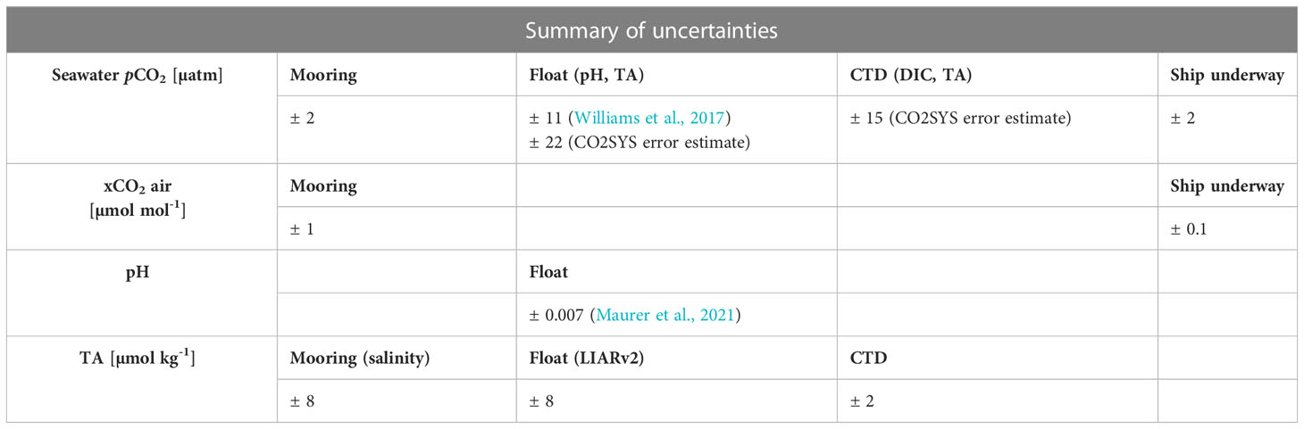
Table 1 Summary of float, mooring, ship underway system and CTD cast bottle measurement and combined uncertainties.

Air-sea fluxes were calculated per equation (2) and mooring air-sea fluxes are from here on called FCO₂^M. For annual flux calculations, daily averaged fluxes were integrated for the calendar year of 2021.

In late April 2021, there was a four day overlap in measurements between SOFS-9 and SOFS-10 sensors, while both moorings were in the water between recovery and deployment (Figure S1). Measurements of pCO₂^M and calculated FCO₂^M of SOFS-9 and SOFS-10 were averaged for this period.

The SOFS moorings are S-tether designs that allow their surface floats to move in large ‘watch circles’. When referring to the mooring location in this manuscript, we refer to the GPS tracked location of the surface buoy, as opposed to the anchor location of the mooring.

2.3 Voyage data and mooring water samples

During the time period of the two moorings discussed here, five research voyages on RV Investigator visited and/or passed the SOTS site (for more information refer to Table S1). RV Investigator is fitted with an automated underway pCO₂ measurement system with an accuracy of ± 2 µatm (Pierrot et al., 2009, Table 1). These data (pCO₂^UW) were used for comparison with pCO₂^M measurements.

During the SOLACE and mooring deployment and recovery voyages DIC and TA samples from CTD casts were collected and analyzed coulometrically and with an (open cell) potentiometric titration, respectively, following standard procedures (Dickson et al., 2007). Regular collection of TA samples during SOTS voyages allowed for the establishment of a robust relationship between TA and salinity at the SOTS site. This linear relationship was derived from samples collected in the upper 100m between 2010 and 2019 and has an error associated with the fit of ~ 8 µmol kg^-1 (Shadwick et al., 2020, Table 1).

$\begin{array}{ll}T{A}^M (\mu mol k{g}^{-1})=39.23*salinity+937.3& (3)\end{array}$

The SOFS mooring surface float houses a modified McLane Remote Access Sampler (RAS), which collects discrete seawater samples at regular intervals. These samples are analyzed for TA^RAS onshore once recovered. Details on quality assurance and QC of these RAS data are published in Shadwick et al. (2020). CTD DIC and TA sample results were used to calculate seawater pH (pH^CTD) with CO2SYS v3.1.1, as described for float data. The calculation of pH from DIC and TA samples introduces an uncertainty that could be avoided in future work if pH was measured directly.

RAS, CTD and mooring TA data were used for comparison to the float estimates of TA^PF. The pCO₂^CTD from CTD samples were calculated with CO2SYSv3.1.1 (Lewis and Wallace, 1998; van Heuven et al., 2011; Sharp et al., 2021) with dissociation constants and nutrient concentrations as outlined for float calculations.

2.4 pCO₂ and air sea flux comparisons between float and mooring

For the most stringent comparison between mooring observations and float estimates, we subsampled the higher resolution mooring data with the following thresholds:

- mooring observations within two days of float profiles

- mooring temperature measurements at 1m and 30m both within 0.3˚C of float temperature measurements averaged over the top 20m

- mooring potential density (sigma theta0) at 1m and 30m both within 0.03 kg m^-3 of float potential density (sigma theta0) averaged over the top 20m

These temperature and potential density thresholds are indicative of well mixed water masses at SOTS (Weeding and Trull, 2014; Shadwick et al., 2015; Jansen et al., 2020; Jansen et al., 2023) and comparable to thresholds used widely for the definition of mixed layer depth (de Boyer Montégut et al., 2004); they are used here to limit the comparison to water masses of similar physical properties. For an overall average seawater pCO₂ of 383 µatm (combining mooring and float data), this temperature difference of 0.3°C would equate to a 5 µatm pCO₂ difference (Takahashi et al., 1993).

For the comparison between pCO₂^M and pCO₂^UW we used the same temperature and potential density criteria but averaged underway data 3h either side of mooring observations and restricted voyage data to within 1° latitude and longitude of mooring location.

To assess the potential influence of distance between mooring and float on the difference in the pCO₂ data (when restricted to temperature and potential density thresholds) we used a model II regression. This reflects the fact that both variables are not controlled and that there is no a priori assumption that there is a dependent variable. Model II regression calculations were performed with the Matlab script lsqfitgm.m (Edward T Peltzer, MBARI, https://www.mbari.org/products/research-software/matlab-scripts-linear-regressions/).

3 Results

In the following sections we compare the individual parameters (pH, TA, etc.) between all available platforms in the area before addressing the main question of pCO₂^PF accuracy. This will put the uncertainties of float estimates and differences between pCO₂^M and pCO₂^PF into context. We will provide uncertainty estimates where available and list these and the results of all comparisons for easier reference in Table 2.

TABLE 2

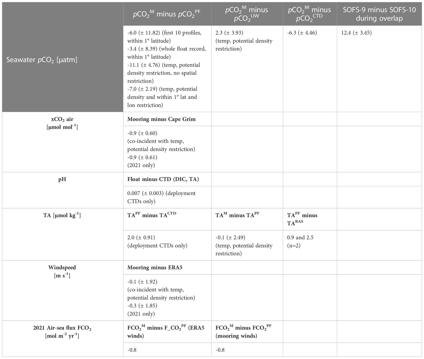
Table 2 Summary of average parameter comparisons between float, mooring, ship underway system and CTD cast bottle samples. Also listed are measurement and combined uncertainties.

3.1 Float pH vs pH calculated from DIC and TA samples

Two CTD casts within 24h of the first three float profiles indicate that pH^{adj corr} compares well to pH^CTD calculated from discrete water samples of DIC and TA collected from the CTD rosette (Figures S2, S4; Table 3). Only float profile data within 5m of each Niskin bottle sample depth were used in the comparison.

TABLE 3

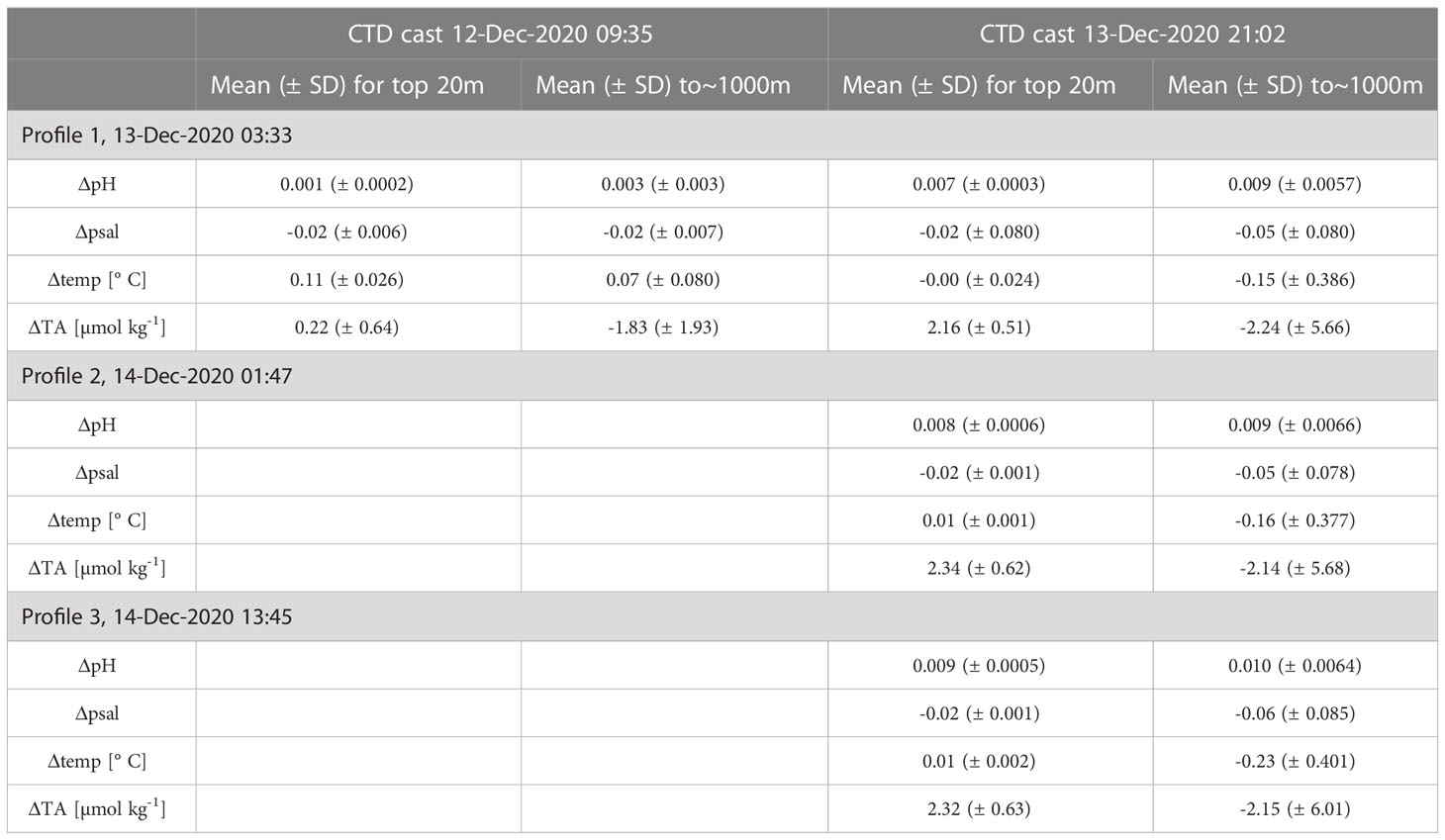
Table 3 pH^{adj corr}, salinity (psal), temperature and TA^PF comparisons to CTD bottle data.

The average difference between pH^{adj corr} of the first profile (13 Dec) and pH^CTD (12 Dec) in the upper 20m was 0.001 (± 0.0002). The average difference over the full depth of the CTD cast, ~ 1000m, was 0.003 (± 0.003). The CTD cast occurred within ~6km of the first float profile. In doing the same comparison between the first profile and a CTD a day later (13 Dec), the mean difference in pH for the top 20m was 0.007 (± 0.0003) and 0.009 (± 0.006) for all samples down to ~ 1000m. The distance between the second cast and the float profile was about 7km (Figures S2, S3; Table 3).

The second and third float profiles occurred on 14 December, ~ roughly 12 hours apart. We compared these two float profiles to CTD data from 13 December, as described above. For the second float profile the mean difference in pH for the top 20m was 0.008 (± 0.0006) and 0.009 (± 0.007) for all samples down to ~ 850m, with a distance of ~13km between float and CTD cast. For the third profile the mean difference in pH for the top 20m was 0.009 (± 0.0005) and 0.010 (± 0.006) for all samples down to ~ 850m and a distance of ~ 18km (Figures S4, S5; Table 3).

3.2 Float TA comparisons

Since computing pCO₂ from float pH measurements requires a second carbon system parameter, i.e. TA, we also compared LIARv2 estimates of TA^PF with TA^CTD from the two CTD casts within 24h of the first three float profiles. We again compared CTD bottle data to float profile data within 5m of each Niskin bottle sample depth. The average difference in TA^PF between the first float profile (13 Dec) minus TA^CTD (12 December) was 0.22 (± 0.64) µmol kg^-1 for the top 20m and -1.83 (± 1.93) µmol kg^-1 for the entire cast to about 1000m. The CTD cast occurred within ~6km of the first float profile. In doing the same comparison between the first profile and CTD cast from 13^th December, the mean difference in TA was 2.16 (± 0.51) µmol kg^-1 for the top 20m and -2.24 (± 5.66) µmol kg^-1 for all samples down to ~ 1000m. The distance between the second cast and the float profile was about 7km (Table 3).

The second and third float profiles occurred on the 14^th of December, roughly 12 hours apart. We compared these two float profiles to CTD data from the 13 December, as described above. For the second float profile the mean difference in TA was 2.34 (± 0.62) µmol kg^-1 for the top 20m and -2.14 (± 5.68) µmol kg^-1 for all samples down to ~ 850m, with a distance of ~13km between float and CTD cast. For the third profile the mean difference in TA was 2.32 (± 0.63) µmol kg^-1 for the top 20m and -2.15 (± 6.01) µmol kg^-1 for all samples down to ~ 850m and a distance of ~ 18km between float and CTD cast (Table 3).

Sharp et al. (2021) included error estimates in their updated CO2SYS Matlab script based on the error propagation analysis by Orr et al. (2018), which calculated TA^PF associated uncertainty of about 8 µatm kg^-1 (0.36%, Table 1). The uncertainty of TA^CTD and TA^RAS is typically ± 2μmol kg^-1 (95% confidence interval, Shadwick et al., 2020, Table 1).

We also compared TA^PF with TA^M estimates and applied the same rules as outlined in the Methods section to limit mooring salinity data (1m and 30m sensors) and TA^M estimates for our comparison. Overall, the difference between TA^M and TA^PF was 0.11 ( ± 2.49) µmol kg^-1 (Table 2), with a maximum difference of ~ 4 µmol kg^-1. Only two RAS samples fell within the restrictions for this comparison (23/6/2021 and 1/7/2021) and the difference between TA^RAS samples and average TA^PF estimates of the top 20m was 2.46 and 0.93 µmol kg^-1, respectively.

3.3 Mooring SOFS-9 pCO₂ vs SOFS-10 pCO₂

In late April 2021, there was a four day overlap between SOFS-9 and SOFS-10 with the moorings about 35km apart (Figures S1, S6). The overlapping seawater temperature sensor data show that the two moorings were exposed to different water masses in the top ~350m, with a temperature difference of about 4˚C and a salinity difference of 0.83. While SOFS-10 was in warmer waters than SOFS-9, it recorded on average seawater pCO₂ of about 12.35 µatm (± 3.45) lower than SOFS-9 (Figure S6), indicating that the difference in pCO₂ was not due to temperature effects but likely due to different water masses, likely warmer, saltier subtropical water, with lower DIC (and thus lower pCO₂; e.g. Pardo et al., 2019), observed by SOFS-10.

3.4 Comparisons between float pCO₂ and mooring, CTD and underway pCO₂

The mean difference between pCO₂^M minus pCO₂^CTD was -6.33 µatm (± 4.46, n=5 CTD samples, Table 2). The CTD casts for this comparison were within<70km of the mooring. We also compared pCO₂^M with pCO₂^UW measurements with the same temperature and potential density criteria as described for pCO₂ and air sea flux. The mean difference between pCO₂^M with pCO₂^UW across the five voyages was 2.29 µatm (± 3.93) with a range of -8.03 µatm to 17.94 µatm (mostly within 60km, with some observations up to ~120km apart, Table 2). Comparisons between the mooring pCO₂ MAPCO2 sensor and the ship underway pCO₂ system in the lab have shown the two systems to be within 2 µatm of each other under ideal conditions (pers. comm. Craig Neill).

Figure 2 shows that between Dec 2020 and May 2021, there were times of close agreement between pCO₂^M and pCO₂^PF, but also times of significant difference. The mean combined uncertainty for pCO₂^PF estimates based on the error propagation routine of the CO2SYS package (Sharp et al., 2021) is 22 µatm (5.6%) for all observations considered here. This assumes a temperature uncertainty of 0.002°C, psal uncertainty of 0.01 (Gray et al., 2018), and no assigned error for nutrients and errors associated with dissociation constants after Orr et al. (2018). Alternatively, if we are to apply a general uncertainty estimate of 2.7% for pCO₂^PF as outlined in Williams et al. (2017), which is based on a top-down uncertainty analysis of float pCO₂ estimates as compared to shipboard underway measurements, this reduces the magnitude of uncertainty to an average of 11 µatm throughout the period of interest. For pCO₂^PF, both error estimate approaches are displayed in Figure 2 as uncertainty envelopes. The pCO₂^M fall within the bounds of uncertainty for pCO₂^PF for the majority of the study period, except for ~90 days in Jan to May 2022 and ~12 days in May 2022 for which they deviated beyond the uncertainty envelopes. Over the entire study period the float drifted in an area of up to ~ 4° Latitude and ~ 3° Longitude from the mooring location (Figure 1). This equates to distances of up to ~ 414km, although over 83% of profiles were within 300km of the mooring. If we restrict the comparison to only the first 10 profiles, within 1˚ latitude from the mooring and use average pCO₂^M 6 hours either side of the float profile, then pCO₂^PF estimates were 6.04 µtam (± 11.82) higher than the average of pCO₂^M. If we extend this to the whole float record and compare mooring data within 6h of the float profiles when both are within 1° latitude, the difference in pCO₂^M minus pCO₂^PF was -3.4 µatm (± 8.39).

FIGURE 2

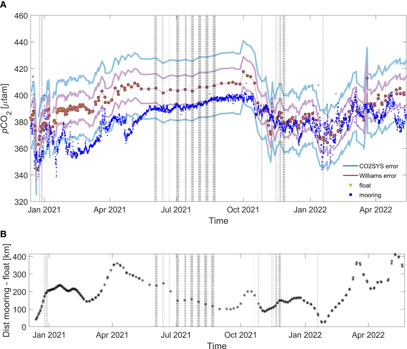
Figure 2 (A) pCO₂^M (dark blue), pCO₂^PF (orange circles) and CO2SYS error propagation (light blue lines) and Williams et al. (2017) (purple lines) error estimates for pCO₂^PF. (B) Distance mooring minus float [km]. Grey shading indicates points that met the temperature and density criteria detailed in the Methods section (in-situ temp within 0.3˚C and potential density within 0.03 kg m^-3 at dates within 2 days).

A recent uncertainty propagation estimate for the marine carbon dioxide system by Orr et al. (2018) showed that dissociation constants K₁ and K₂ contribute the most to the combined standard uncertainty. Therefore we also calculated pCO₂^PF with those recently presented by Schockman and Byrne (2021) which are experimentally determined with spectrophotometric methods and evaluated with shipboard and laboratory data. The pCO₂^PF using the K₁ and K₂ constants by Schockman and Byrne (2021) are ~4 µatm higher than those calculated using constants by Lueker et al. (2000), increasing the gap between pCO₂^M and pCO₂^PF further. To remain consistent with other float-based pCO₂ estimates available in this region and used within other studies (Johnson et al., 2017; Gray et al., 2018; Johnson et al., 2022), for the remainder of this work, we therefore focus on calculations based on constants by Lueker et al. (2000) but note the size of the uncertainty introduced by the different choices in K₁ and K₂ constants. We also note that the application of the Williams et al. (2017) bias correction reduces pCO₂^PF estimates by ~5.9 µatm (± 0.29) over the entire float record, or in other words, without the application of said bias correction the gap between pCO₂^M and pCO₂^PF would be larger.

The comparison between the overlapping SOFS-9 and SOFS-10 at close proximity (~35km) shows that limiting comparisons by distance alone may not be enough. We therefore used temperature and potential density as criteria for comparable water masses. Of the 242 float profiles that occurred during the time covered in this study, only 27 profiles passed the temperature and potential density criteria outlined in the Methods section, highlighting the great spatial variability in seawater properties in this region. Considering only the subset of data that passed these criteria, pCO₂^PF was always higher than pCO₂^M (overall mean difference of -11.06 µatm ± 4.76, Table S2). This was most noticeable for the winter period of 2021 (grey shading Figure 2A). Application of the Takahashi temperature correction (Takahashi et al., 1993) before comparing pCO₂^PF to pCO₂^M for this subset of data makes little difference to the average discrepancy (– 11.17 µatm ± 7.74). Diurnal variations in pCO₂ could contribute to the discrepancy between pCO₂^PF and pCO₂^M comparisons when averaging pCO₂^M either side of float profile times. A comparison with mooring observations 2 days either side of the float profile averages this diurnal signal and therefore has an overall small effect on the comparisons. We also calculated the overall mean difference between pCO₂^M and pCO₂^PF estimate with the same temperature and potential density criteria, but 6 hour (-10.48 µatm ± 3.95) and 3h (-9.92 µatm ± 4.04) either side of the float profile and note that this does not make a statistically distinguishable difference.

To investigate the influence of distance between the mooring and float on the pCO₂ differences under the most stringent comparison conditions (temperature and potential density), we calculated a Model II regression between the difference in pCO₂ and the distance in km between mooring and float for those data only (Figure 3). Mooring pCO₂^M that met the temperature, potential density and time criteria (outlined in the Methods) were averaged before subtracting pCO₂^PF. Float profiles included in this regression were south and north of the mooring locations (Figure 4), yet the differences between pCO₂^M and pCO₂^PF were all negative, unlike the differences between pCO₂^M and pCO₂^UW described above, which were both negative and positive.

FIGURE 3

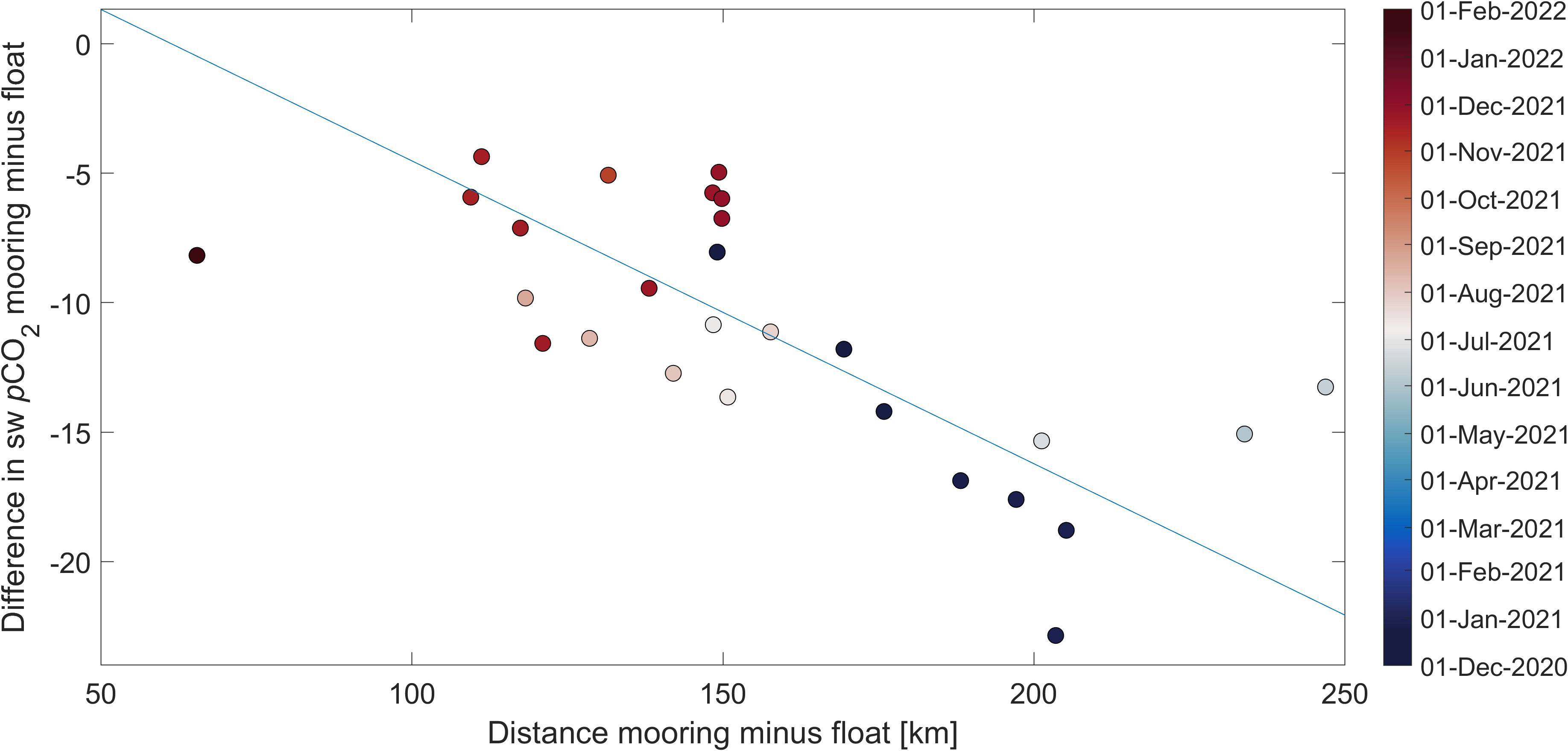
Figure 3 Model II regression for distance between mooring and float (km) and difference in pCO₂^M minus pCO₂^PF (µatm) for data that met the most stringent criteria for being in comparable water masses (see Methods). Slope = - 0.12 ( ± 0.02), y-intercept = 7.17 ( ± 2.99), r² = -0.69, noting that for a Model II regression the correlation coefficient is a measure of the linearity of the data and not how well the line fits the data.

FIGURE 4

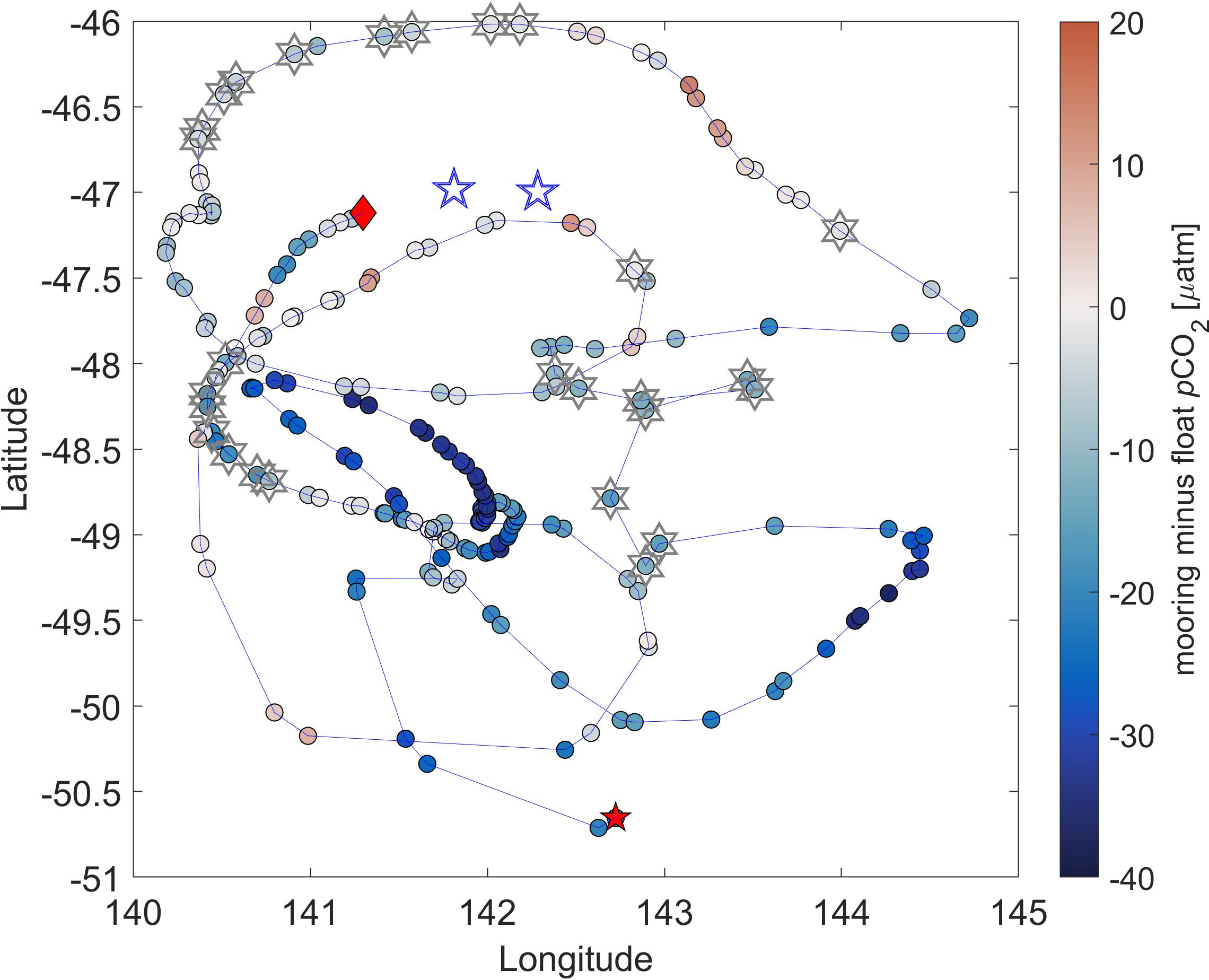
Figure 4 Float track with overlaid difference in pCO₂ (mooring observations within 2 days of float profiles minus float estimates in µatm, not distance corrected). Mooring locations are indicated by the blue star symbols, the start of the float track is indicated by a red diamond, the final profile included in this study is marked by a red star. Float profiles that met the temperature and potential density criteria are marked by superimposed grey hexagrams.

There is a clear signal that the farther away the float was from the mooring, the larger the difference in pCO₂. While the float moved east and west around the mooring, it predominantly moved south, with only one short excursion to the north (Figure 4). Only 10 profiles (November 2021) met the temperature and potential density criteria and were within 1° latitude and 1° longitude of the moorings. The average difference in pCO₂ under those conditions was -7.01 µatm (± 2.19). For these profiles (unlike the other comparisons) the float measured higher temperatures in the top 20m compared to the mooring sensors at 1m and 30m, and therefore applying the temperature correction to pCO₂^PF reduces the discrepancy to -3.27 µatm (± 2.57).

To investigate whether there were any co-varying properties along with distance, we overlaid float dissolved oxygen, chlorophyll (Chl a), mixed layer depth, nitrate concentration and windspeeds at the location of the float profiles (not shown). However, none of these parameters correlated with the distance to the mooring. There was also no correlation between these parameters and the difference in seawater pCO₂ between mooring and float. Figure 4 shows the float track in relation to the mooring locations colored with the ΔpCO₂. To illustrate the difference in pCO₂ for all float profiles, we averaged pCO₂^M within 2d of float profiles, but not taking into account temperature and potential density differences (Figure 4). This highlights that the greatest differences in pCO₂ are seen in profiles that occurred south of the mooring, which occurred during autumn months. In Figure 4 we also marked those profiles that additionally met the temperature and potential density criteria with grey hexagons, which shows that the profiles with the overall largest (negative) difference between pCO₂^M and pCO₂^PF did not meet temperature and density criteria.

If the majority of the difference in mooring and float pCO₂ was attributable to distance, then the two results could be brought in line via the above regression. We therefore applied the slope and intercept to all pCO₂^PF data, as per equation (4):

$\begin{array}{ll}regressed float pC{O}_{2 }= d_{m-f}*(-0.12)+7.17+pC{O}_2{}_{}^{PF}& (4)\end{array}$

Where d_m-f is the distance (km) between mooring and float. This brings pCO₂^PF closer in line with pCO₂^M for parts of the time period discussed here, particularly during the autumn/winter period of 2021 (Figure 5B). The intention of this was not to “correct” pCO₂^PF estimates but to test the theory that some of the difference in pCO₂ is based on a true (predominantly latitudinal) distance gradient.

FIGURE 5

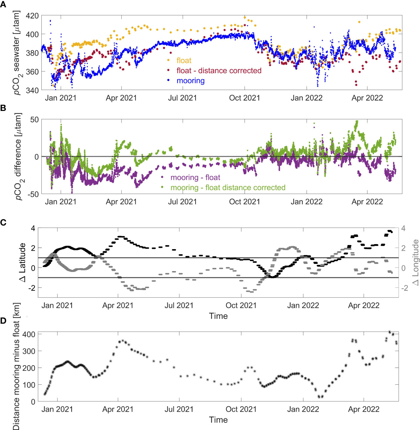
Figure 5 (A) pCO₂^M (blue) compared to pCO₂^PF for the top 20m (orange) and after application of the distance regression (dark red). (B) Difference in pCO₂ mooring minus float, for pCO₂^PF (purple) and distance corrected float pCO₂ (light green). For the comparisons in (A, B) all mooring data/mooring minus float data within 2 days of float profiles were plotted. (C) ΔLatitude and ΔLongitude mooring minus float profiles within 2 days of profiles; grey horizontal lines demark ± 1˚ Latitude/Longitude. (D) Distance mooring minus float [km].

3.5 Float vs mooring air-sea flux estimates and associated input parameters

The annual FCO₂^M for the calendar year 2021, without limiting the data otherwise, was -1.68 (± 0.004) mol m^-2 yr^-1 compared to FCO₂^PF -0.89 (± 0.003) mol m^-2 yr^-1 (Figures 6; Figure S8). Most notable are short periods of outgassing seen in the float estimates during austral autumn 2021 (April and May), when the mooring estimates show significant CO₂ uptake instead. This was also the time period of the largest difference in seawater temperature and salinity (Figure 6), when a warmer, saltier water mass that extended to ~ 350m was recorded by SOFS-10 for about a month (Figure S6). Both mooring and float agree, however, on periods of outgassing in austral spring 2021 (Sept and Oct).

FIGURE 6

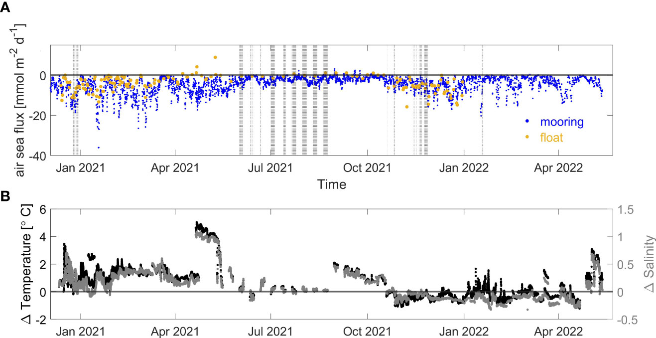
Figure 6 (A) Mooring (blue) and float (orange) air-sea fluxes (mmol m^-2 d^-1). (B) Mooring 1m temperature/salinity minus average top 20m float temperature/salinity (± 2 days). Grey shading indicates points that met the temperature and density criteria detailed in the Methods section (in-situ temp within 0.3˚C and potential density within 0.03 kg m^-3 at dates within 2 days).

Since squared windspeed factors into air-sea flux calculations we also calculated air-sea fluxes for the float with windspeed observations from the mooring instead of ERA5 windspeeds. For this we used the average windspeed mooring data 3h either side of the float profile time (Figure S8) and equation 2, but with the same scaling factor for the gas transfer coefficient. Mooring windspeed is not assumed to be more accurate than ERA5 winds for the location of the float profile (a comparison between ERA5 winds and moorings winds is shown in Figure S7), rather this calculation is to visualize the effect of choosing different windspeed products on air-sea flux calculations. The mean difference between mooring windspeed minus ERA5 windspeed at the float locations for 2021 was -0.27 (± 1.79) m s^-1, with a range of 0.02 to 5.47 m s^-1 and no bias over time. Using mooring windspeed for the float calculations resulted in a near identical annual flux of -0.88 (± 0.003) mol m^-2 yr^-1. To exemplify the impact of pCO₂^PF uncertainties as compared to the impact of the choice of windspeed, we calculated FCO₂^PF with a Monte Carlo approach (1000 simulations) using a mean pCO₂ uncertainty of - 11.2 µatm (± 7.7), - 7 µatm (± 2.2) and – 3.3 µatm (± 2.6) for the calendar year 2021, which resulted in an air-sea flux of -1.92 mol m^-2 yr^-1 (± 0.004 for ERA5 winds, vs -1.89 mol m^-2 yr^-1 ± 0.004 for mooring windspeeds), - 1.54 mol m^-2 yr^-1 (± 0.004 ERA5, -1.51 mol m^-2 yr^-1 ± 0.004 mooring windspeed) and – 1.20 mol m^-2 yr^-1 (± 0.003 ERA5, - 1.18 mol m^-2 yr^-1 ± 0.003 mooring windspeed), respectively; indicating that the uncertainty in pCO₂^PF has a far great impact on air-sea flux estimates than the choice of windspeed product.

4 Discussion

The aim of this work was to evaluate the accuracy of pCO₂^PF estimates beyond the initial in water comparisons with CTD samples at the time of deployment. For this we drew on direct pCO₂ observations from two moorings, as well as shipboard underway systems, and estimates from discrete CTD samples, and the proximity of a BGC Argo float to the SOTS mooring site for more than a year.

4.1 Comparisons close in space

The spatial variability in this region of the Southern Ocean is well known and makes direct comparison of drifting float measurements and fixed-mooring observations difficult. A comparison based purely on time is not appropriate for periods when the float was up to ~360km away and/or “up- or downstream” of the mooring site. Ideally, only measurements in the same water mass would be used. Therefore, we started by comparing observations between platforms when they were close in time and space first, e.g. CTD casts shortly after the deployment of the float.

The initial comparison between CTD samples and float measurements showed that the float pH sensor was calibrated and functioning correctly at the time of deployment. Extending the comparison to the first 10 profiles, which were within 1˚ latitude from the mooring, pCO₂^PF estimates were about 6.0 µtam (± 11.82) higher than mooring observations within 6h of each profile. This agrees with previous reports (using various methods) of a bias in float pCO₂ estimates of about 4 – 8 µatm higher (Gray et al., 2018; Williams et al., 2018; Bushinsky et al., 2019; Long et al., 2021; Wu and Qi, 2022). It is also important to note that Maurer et al. (2021) stated that float pH measurements adjusted according to the method described in their paper (and applied in this study) are accurate to approximately 0.007 (based on validation efforts which compared adjusted float pH to shipboard data taken alongside deployment). This also matches our comparison between float pH^{adj corr} and pH^CTD estimates at the time of deployment. An uncertainty of 0.007 pH units roughly equates to 7 µatm pCO₂, which is only ~ 1 µatm higher than the magnitude of the difference between mooring and the first 10 float profiles close in space reported in this study. Gray et al. (2018) (based on Williams, 2017), estimated pCO₂^PF uncertainty to be in the order of 2.9%, which equates to 11 µatm for the entire observation period presented here. Combined uncertainties after Orr et al. (2018) were about twice as large (~ 22 µatm, 5.6% relative uncertainty, Table 1). Therefore, we emphasize that comparing pCO₂^PF to pCO₂^M close in space and time yields differences that are well within the limits of stated pH sensor capabilities and pCO₂ estimate uncertainties. This was also true when we compared the whole float record (over a year) to mooring data, while applying the latitude and time restrictions (see below).

4.2 Comparisons in comparable water masses

It is not clear how much of the observed difference in pCO₂ over the course of the year can be attributed directly to uncertainty in float estimates. As from the overlapping mooring observations, pCO₂ can be significantly different if water masses with genuinely different characteristics are encountered. We therefore used temperature and potential density as criteria for when mooring and float were in comparable water masses. The difference between pCO₂^M and pCO₂^PF when only looking at data restricted with this water mass criteria was around 11 µatm (Table 2), which is within stated uncertainties. Mean uncertainty estimates of TA^PF were about 8 µmol kg^-1, which is larger than the 5 µmol kg^-1 reported by Williams et al. (2018). Comparison between TA^PF, TA^M and CTD samples were well within these uncertainties. A relative uncertainty in TA of 0.4% (based on the LIARv2 TA) would translate to a relative uncertainty of 0.4% in pCO₂ (Dickson and Riley, 1978). Thus, the difference in pCO₂^PF is not predominantly due to uncertainties in TA^PF, but could be attributed to uncertainties in seawater carbonate system thermodynamics as well as uncertainties in the adjusted float pH measurements, which would also include any uncertainty in measured dissolved oxygen concentration used to adjust the pH and used for LIARv2 estimates of TA (Johnson et al., 2016; Johnson et al., 2017; Williams et al., 2017; Gray et al., 2018). Orr et al. (2018) found combined uncertainties in carbon system parameter estimates to be largely driven by uncertainties in dissociation constants. We therefore tried the most commonly used K₁ K₂ constants by Lueker et al. (2000), as well as more recently refined constants by Schockman and Byrne (2021). The pCO₂ ^PF estimates were about 4 µatm higher when using constants by Schockman and Byrne (2021) and therefore increased rather than reduce the difference between pCO₂^M and pCO₂^PF.

The comparison of pCO₂^M and pCO₂^PF when restricted to temperature and potential density criteria revealed a relationship of increasing difference in pCO₂ with increasing distance between mooring and float. While application of a calculated distance regression reduced the gap between pCO₂^PF and pCO₂^M, there were times when the opposite was true, particularly during the autumn of 2022 (Figure 5A, in late March 2022), when the float drifted up to ~ 400km away from the mooring yet the distance corrected float pCO₂ disagreed more with pCO₂^M than with the uncorrected pCO₂^PF. This indicates that distance-associated variability is not the only factor contributing to the observed difference between pCO₂^PF and pCO₂^M.

4.3 The importance of spatial and temporal variability

For most of the study period, mooring seawater temperature in the top 30m was higher than float averages for the top 20m. Thus, the expected change in pCO₂ (Takahashi et al., 1993) for the difference in seawater temperature would not explain the disagreement, but in fact emphasize it (note the above mentioned exception for the November 2021 period). A latitudinal gradient in seawater pCO₂ in this part of the SAZ has recently been shown from ship-based repeat measurements along a transect from Tasmania to Antarctica (Brandon et al., 2022). Data presented by Brandon et al. (2022) show a southward increase in seawater pCO₂ of up to 25 µatm for the latitudinal range between mooring and float encountered in the study period. They attributed this gradient in part to an increasing influence of subtropical waters in the SOTS region of the SAZ. Temperature profiles from both mooring and float for the time period where their pCO₂ data disagree the most (February to October 2021) also indicate that there were water masses coming past the moorings that were not encountered by the float (e.g. May 2021, Figure 7). As discussed above, the difference in pCO₂ between SOFS-9 and SOFS-10 when they encountered different water masses, was ~12 µatm, highlighting the importance of such events for surface pCO₂ variability.

FIGURE 7

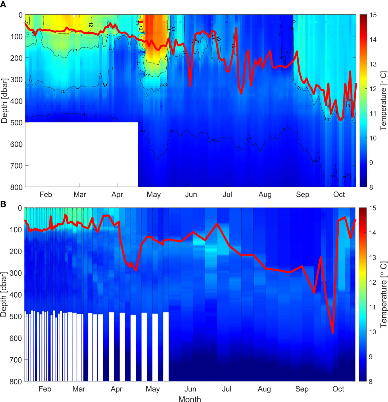
Figure 7 (A) Mooring and (B) float (MLD in red, 0.3°C absolute difference to 10m reference depth) temperature contours for the period of largest disagreement in pCO₂.

Bushinsky et al. (2019) used high-resolution ocean biogeochemical models to investigate the underlying cause of the differences between float and ship-based estimates and found that some of the difference can be explained by spatial and temporal sampling differences. This has more recently been confirmed, particularly for the SAZ, by Djeutchouang et al. (2022). By comparing the surface pCO₂ of a high-resolution coupled physical and biogeochemical model with reconstructed pCO₂ after sampling the model in time and space the way a BGC float and ship would, they show that reducing the uncertainty in the reconstructed pCO₂ depended on how well the spatial and meridional gradients and the temporal, seasonal and intra-seasonal pCO₂ variability was resolved. High temporal sampling resolution (ideally at least daily) and a meridional gradient resolving sampling strategy were best equipped to achieve that (Djeutchouang et al., 2022). In other words, a moored observation platform with high frequency sampling, resolves the seasonal and intra-seasonal variability well, and also captures mesoscale variability but it does not resolve the meridional gradient, which is particularly important in the SAZ and could explain the discrepancies between pCO₂^M and pCO₂^PFas the float drifted away.

Between 10 and 25% of the uncertainty in float based carbon flux estimate was previously attributed to the low temporal resolution of 10-day cycling which may frequently miss short-lived but significant changes in mixed-layer depth due to storms and wind-stress and the associated changes in up-welling of carbon-rich deep waters and this was found to be particularly true for the SAZ (Monteiro et al., 2015; Nicholson et al., 2022). In our study, positive float-based air-sea fluxes (i.e. outgassing) between April and June 2021 - and to a lesser degree in September 2021 – suggest that the float measured regional events which the mooring did not, and that these outgassing events may be possibly genuine oceanographic features.

The 3 – hourly resolution mooring observations show how variable seawater surface pCO₂ is in this region of the SAZ (Figures 5, 6), with subtropical water masses reaching the site intermittently. If we limit the comparison of the whole pCO₂^PF data to mooring data within 2d either side of float profiles, 0.3°C temperature and 0.03 kg m^-3 potential density restriction and a latitudinal and longitudinal difference of less than 1˚, we find a mean difference in seawater pCO₂ of -7.0 (± 2.19) µatm, indicating again a generally higher pCO₂ estimate from the float, but well within stated pCO₂ uncertainty estimates. Based on the comparison with previous findings and the potentially large uncertainty of pCO₂^PF, we find that the difference between pCO₂^PF and pCO₂^M observed in this study appears to be a combination of a potential small positive bias in pCO₂^PF estimates, a zonal gradient in seawater surface pCO₂ in this sector of the SAZ, and relatively fine scale spatial and temporal variability.

5 Conclusion

Understanding and observing the Southern Ocean carbon uptake is of great interest in the face of continued rise in anthropogenic carbon emissions. Due to the dynamic and complex nature of the processes that govern the uptake and outgassing of carbon in this region, sufficient temporal and spatial coverage in carbon system measurements is vital. Autonomous platforms such as BGC Argo profiling floats address an important gap in carbon system observations in the Southern Ocean and have greatly expanded spatial and temporal coverage. And, while spatiotemporal coverage may be limited from a single float, through the continued expansion of the BGC Argo array a cohesive dataset is emerging which is already providing key information on biogeochemical cycling on seasonal and even diel timescales (Johnson and Bif, 2021; Johnson et al., 2022; Stoer and Fennel, 2022). However, the absolute accuracy of pCO₂ estimates from pH measurements on these floats is still under debate, with a number of factors contributing to overall uncertainties. To address this question, we capitalized on the opportunity of a year of float profiles in the vicinity of the long-term Southern Ocean Time Series observatory. Comparing measurements from a drifting float with those from two fixed-point mooring sensors, we found pCO₂^PF estimates to be ~ 11 µatm higher than pCO₂^M, when only comparing measurements within strict temperature and density criteria. Further limiting the comparison between pCO₂^PF and pCO₂^M to a spatial limit of 1° latitude and 1° longitude resulted in a difference of ~ 3-7 µatm. Both these differences are well within float-based pCO₂ estimate uncertainties with the observed positive bias contributing significantly to this uncertainty. Therefore, the differences in pCO₂ estimates of the drifting BGC Argo float and pCO₂ observations from two fixed-moorings over the course of a year are a combination of pCO₂ estimate uncertainties and spatial and temporal variability within this region of the SAZ. Continued validation efforts, using measurements with known and sufficient accuracy, are vital in the continued assessment of pCO₂^PF, especially in a highly dynamic region such as the SAZ, and our findings need to be validated in other areas of the global oceans. This work reinforces that, even when considering observational uncertainty, the Indian Ocean sector of the subantarctic zone is a carbon sink on an annual basis, but with a latitudinal gradient that may encompass areas of outgassing over the winter season.

Data availability statement

The datasets presented in this study can be found in online repositories. The names of the repository/repositories and accession number(s) can be found below: SOFS mooring sensor and water sample data is available from the Australian Ocean Data Network (AODN) https://portal.aodn.org.au/. SOFS mooring pCO₂^M and pCO₂^M_air data is accessible from the Ocean Carbon and Acidification Data System (OCADS). (Sutton et al., 2014b). from https://www.ncei.noaa.gov/access/ocean-carbon-data-system/oceans/Moorings/SOFS.html. Argo float data is available from the Argo Global Data Assembly Center (GDAC). Data were last downloaded on 21/10/2022 (Argo, 2000). Voyage CTD water sample data is available from SOTS annual sample reports, available from https://catalogue-imos.aodn.org.au/geonetwork/srv/eng/catalog.search#/metadata/afc166ce-6b34-44d9-b64c-8bb10fd43a07 Voyage underway pCO₂UW data is accessible from the IMOS Ships of Opportunity (SOOP) thredds server: https://thredds.aodn.org.au/thredds/catalog/IMOS/SOOP/SOOP-CO2/VLMJ_Investigator/catalog.html Cape Grim atmospheric xCO2 data was downloaded from https://www.csiro.au/en/research/natural-environment/atmosphere/Latest-greenhouse-gas-data. ERA5 windspeed and mean sea level pressure data was accessed from Copernicus Climate Change Service (C3S) Climate Data Store, (Hersbach et al., 2018) (ERA5 hourly data on single levels from 1940 to present). World Ocean Atlas nutrient data was downloaded from https://www.ncei.noaa.gov/thredds-ocean/catalog/ncei/woa/phosphate/all/1.00/catalog.html, (Boyer et al., 2018).

Author contributions

Conceptualization: CW-E, ES. Data acquisition and QC: ES, PJ, CS, CW-E, AS, TM. Methodology: CW-E, CS, TM. Writing—original draft preparation: CW-E. Writing—review and editing: all authors. All authors have read and agreed to the published version of the manuscript.

Funding

This project received funding from the Australian Government as part of the Antarctic Science Collaboration Initiative program. The air-sea CO₂ moored observations are supported by NOAA’s Pacific Marine Environmental Laboratory. This is PMEL contribution 5514.

Acknowledgments

Operated by a consortium of institutions as an unincorporated joint venture, with the University of Tasmania as Lead Agent. We acknowledge support from the University of Tasmania (UTAS), Australian Antarctic Program Partnership (AAPP), Bureau of Meteorology (BoM), Marine National Facility (MNF). SOTS is a member of the OceanSITES global network of time series observatories (www.OceanSITES.org). Thanks to Tom Trull for providing helpful comments that improved an earlier version of the manuscript. The BGC-Argo data used for this analysis were downloaded on 21/10/2022, http://doi.org/10.17882/42182#96550. These data were collected and made freely available by the International Argo Program and the national programs that contribute to it. (https://argo.ucsd.edu, https://www.ocean-ops.org). The Argo Program is part of the Global Ocean Observing System (Argo, 2000). Argo (2000). Argo float data and metadata from Global Data Assembly Centre (Argo GDAC). SEANOE. https://doi.org/10.17882/42182. We used the Matlab package cmocean for figure colormaps (Thyng et al., 2016).

Conflict of interest

The authors declare that the research was conducted in the absence of any commercial or financial relationships that could be construed as a potential conflict of interest.

Publisher’s note

All claims expressed in this article are solely those of the authors and do not necessarily represent those of their affiliated organizations, or those of the publisher, the editors and the reviewers. Any product that may be evaluated in this article, or claim that may be made by its manufacturer, is not guaranteed or endorsed by the publisher.

Supplementary material

The Supplementary Material for this article can be found online at: https://www.frontiersin.org/articles/10.3389/fmars.2023.1231953/full#supplementary-material

References

Argo (2000). Argo Float Data and Metadata from Global Data Assembly Centre (Argo GDAC: SEANOE).

Google Scholar

Bakker D. C., Pfeil B., Landa C., Metzl N., O'Brien K., Olsen A., et al. (2016). A multi-decade record of high-quality fCO₂ data in version 3 of the Surface Ocean CO₂ Atlas (SOCAT). Earth System Sci. Data 8 (2), 383–413. doi: 10.5194/essd-8-383-2016

CrossRef Full Text | Google Scholar

Boyer T. P., Garcia H. E., Locarnini R. A., Zweng M. M., Mishonov A. V., Reagan J. R., et al. (2018) World Ocean Atlas 2018. Available at: https://www.ncei.noaa.gov/archive/accession/NCEI-WOA18 (Accessed 03/02/2022).

Google Scholar

Brandon M., Goyet C., Touratier F., Lefèvre N., Kestenare E., Morrow R. (2022). Spatial and temporal variability of the physical, carbonate and CO₂ properties in the Southern Ocean surface waters during austral summer, (2005-2019). Deep Sea Res. Part I: Oceanographic Res. Papers 187, 103836. doi: 10.1016/j.dsr.2022.103836

CrossRef Full Text | Google Scholar

Bushinsky S. M., Landschützer P., Rödenbeck C., Gray A. R., Baker D., Mazloff M. R., et al. (2019). Reassessing Southern Ocean air-sea CO₂ flux estimates with the addition of biogeochemical float observations. Global Biogeochemical Cycles 33 (11), 1370–1388. doi: 10.1029/2019GB006176

PubMed Abstract | CrossRef Full Text | Google Scholar

Carter B., Feely R., Williams N., Dickson A., Fong M., Takeshita Y. (2018). Updated methods for global locally interpolated estimation of alkalinity, pH, and nitrate. Limnology Oceanography: Methods 16 (2), 119–131. doi: 10.1002/lom3.10232

CrossRef Full Text | Google Scholar

Carter B., Radich J., Doyle H., Dickson A. (2013). An automated system for spectrophotometric seawater pH measurements. Limnology Oceanography: Methods 11 (1), 16–27. doi: 10.4319/lom.2013.11.16

CrossRef Full Text | Google Scholar

Crisp D., Dolman H., Tanhua T., McKinley G. A., Hauck J., Bastos A., et al. (2022). How well do we understand the land-ocean-atmosphere carbon cycle? Rev. Geophysics 60 (2), e2021RG000736. doi: 10.1029/2021RG000736

CrossRef Full Text | Google Scholar

de Boyer Montégut C., Madec G., Fischer A. S., Lazar A., Iudicone D. (2004). Mixed layer depth over the global ocean: An examination of profile data and a profile-based climatology. J. Geophysical Research: Oceans 109 (C12), 1–20. doi: 10.1029/2004JC002378

CrossRef Full Text | Google Scholar

Dickson A. G. (1990). Thermodynamics of the dissociation of boric acid in synthetic seawater from 273.15 to 318.15 K. Deep Sea Res. Part A. Oceanographic Res. Papers 37 (5), 755–766. doi: 10.1016/0198-0149(90)90004-F

CrossRef Full Text | Google Scholar

Dickson A., Riley J. (1978). The effect of analytical error on the evaluation of the components of the aquatic carbon-dioxide system. Mar. Chem. 6 (1), 77–85. doi: 10.1016/0304-4203(78)90008-7

CrossRef Full Text | Google Scholar

Dickson A. G., Sabine C. L., Christian J. R. (2007). Guide to Best Practices for Ocean CO₂ Measurements (Sidney, Canada: PICES Special Publication 3, North Pacific Marine Science Organization).

Google Scholar

Djeutchouang L. M., Chang N., Gregor L., Vichi M., Monteiro P. (2022). The sensitivity of pCO₂ reconstructions to sampling scales across a Southern Ocean sub-domain: a semi-idealized ocean sampling simulation approach. Biogeosciences 19 (17), 4171–4195. doi: 10.5194/bg-19-4171-2022

CrossRef Full Text | Google Scholar

Ellwood M., Trull W. T., Antoine D., Kloser R., Masque P. (2021) MNF Voyage Summary - IN2020_V08. Available at: https://www.marine.csiro.au/data/reporting/get_file.cfm?eov_pub_id=1585.

Google Scholar

Fay A. R., Gregor L., Landschützer P., McKinley G. A., Gruber N., Gehlen M., et al. (2021). SeaFlux: harmonization of air–sea CO₂ fluxes from surface pCO₂ data products using a standardized approach. Earth Syst. Sci. Data 13 (10), 4693–4710. doi: 10.5194/essd-13-4693-2021

CrossRef Full Text | Google Scholar

Fay A. R., Lovenduski N. S., McKinley G. A., Munro D. R., Sweeney C., Gray A. R., et al. (2018). Utilizing the Drake Passage Time-series to understand variability and change in subpolar Southern Ocean pCO₂. Biogeosciences 15 (12), 3841–3855. doi: 10.5194/bg-15-3841-2018

CrossRef Full Text | Google Scholar

Friedlingstein P., Jones M. W., O'Sullivan M., Andrew R. M., Bakker D. C., Hauck J., et al. (2022). Global carbon budget 2021. Earth System Sci. Data 14 (4), 1917–2005. doi: 10.5194/essd-14-1917-2022

CrossRef Full Text | Google Scholar

Froehlicher T. L., Sarmiento J. L., Paynter D. J., Dunne J. P., Krasting J. P., Winton M. (2015). Dominance of the Southern Ocean in anthropogenic carbon and heat uptake in CMIP5 models. J. Climate 28 (2), 862–886. doi: 10.1175/JCLI-D-14-00117.1

CrossRef Full Text | Google Scholar

Gray A. R., Johnson K. S., Bushinsky S. M., Riser S. C., Russell J. L., Talley L. D., et al. (2018). Autonomous biogeochemical floats detect significant carbon dioxide outgassing in the high-latitude Southern Ocean. Geophysical Res. Lett. 45, 9049–9057. doi: 10.1029/2018GL078013

CrossRef Full Text | Google Scholar

Gruber N., Clement D., Carter B. R., Feely R. A., Van Heuven S., Hoppema M., et al. (2019). The oceanic sink for anthropogenic CO₂ from 1994 to 2007. Science 363 (6432), 1193–1199. doi: 10.1126/science.aau5153

PubMed Abstract | CrossRef Full Text | Google Scholar

Gruber N., Gloor M., Mikaloff Fletcher S. E., Doney S. C., Dutkiewicz S., Follows M. J., et al. (2009). Oceanic sources, sinks, and transport of atmospheric CO₂. Global Biogeochemical Cycles 23 (1), 1–21. doi: 10.1029/2008GB003349

CrossRef Full Text | Google Scholar

Helm K. P., Bindoff N. L., Church J. A. (2011). Observed decreases in oxygen content of the global ocean. Geophysical Res. Lett. 38, L23602. doi: 10.1029/2011GL049513

CrossRef Full Text | Google Scholar

Hersbach H., Bell B., Berrisford P., Biavati G., Horányi A., Muñoz Sabater J., et al. (2018). ERA5 hourly data on single levels from 1979 to present. Copernicus climate change service (c3s) climate data store (cds) 10(10.24381). doi: 10.24381/cds.adbb2d47 Accessed on 27/09/2022.

CrossRef Full Text | Google Scholar

Jansen P., Shadwick E. H., Trull T. W. (2022). Southern Ocean Time Series (SOTS): Multi-year Gridded Product Version 1.1 (Australia: CSIRO). doi: 10.26198/gfgr-fq47

CrossRef Full Text | Google Scholar

Jansen P., Weeding B., Shadwick E. H., Trull T. W. (2020). Southern Ocean Time Series (SOTS) Quality Assessment and Control Report Temperature Records Version 1.0 (Australia: CSIRO). doi: 10.26198/gfgr-fq47

CrossRef Full Text | Google Scholar

Jansen P., Wynn-Edwards C. A., Shadwick E. H., Trull T. W. (2023). Southern Ocean Time Series (SOTS) Quality Assessment and Control Report Oxygen Records 2009-2021. Version 1.0 (Australia: CSIRO). doi: 10.26198/1te4-jq81

CrossRef Full Text | Google Scholar

Johnson K. S., Bif M. B. (2021). Constraint on net primary productivity of the global ocean by Argo oxygen measurements. Nat. Geosci. 14 (10), 769–774. doi: 10.1038/s41561-021-00807-z

CrossRef Full Text | Google Scholar

Johnson K. S., Jannasch H. W., Coletti L. J., Elrod V. A., Martz T. R., Takeshita Y., et al. (2016). Deep-Sea DuraFET: A pressure tolerant pH sensor designed for global sensor networks. Analytical Chem. 88 (6), 3249–3256. doi: 10.1021/acs.analchem.5b04653

CrossRef Full Text | Google Scholar

Johnson K. S., Mazloff M. R., Bif M. B., Takeshita Y., Jannasch H. W., Maurer T. L., et al. (2022). Carbon to nitrogen uptake ratios observed across the Southern Ocean by the SOCCOM profiling float array. J. Geophysical Research: Oceans 127 (9), e2022JC018859. doi: 10.1029/2022JC018859

CrossRef Full Text | Google Scholar

Johnson K. S., Plant J. N., Coletti L. J., Jannasch H. W., Sakamoto C. M., Riser S. C., et al. (2017). Biogeochemical sensor performance in the SOCCOM profiling float array. J. Geophysical Research: Oceans 122 (8), 6416–6436. doi: 10.1002/2017JC012838

CrossRef Full Text | Google Scholar

Keppler L., Landschützer P. (2019). Regional wind variability modulates the Southern Ocean carbon sink. Sci. Rep. 9 (1), 1–10. doi: 10.1038/s41598-019-43826-y

PubMed Abstract | CrossRef Full Text | Google Scholar

Landschützer P., Gruber N., Haumann F. A., Rödenbeck C., Bakker D. C., Van Heuven S., et al. (2015). The reinvigoration of the Southern Ocean carbon sink. Science 349 (6253), 1221–1224. doi: 10.1126/science.aab2620

PubMed Abstract | CrossRef Full Text | Google Scholar

Landschützer P., Tanhua T., Behncke J., Keppler L. (2023). Sailing through the southern seas of air–sea CO₂ flux uncertainty. Philos. Trans. R. Soc. A 381 (2249), 20220064. doi: 10.1098/rsta.2022.0064

CrossRef Full Text | Google Scholar

Langlais C., Lenton A., Matear R., Monselesan D., Legresy B., Cougnon E., et al. (2017). Stationary Rossby waves dominate subduction of anthropogenic carbon in the Southern Ocean. Sci. Rep. 7 (1), 17076. doi: 10.1038/s41598-017-17292-3

PubMed Abstract | CrossRef Full Text | Google Scholar

Lee K., Kim T.-W., Byrne R. H., Millero F. J., Feely R. A., Liu Y.-M. (2010). The universal ratio of boron to chlorinity for the North Pacific and North Atlantic Oceans. Geochimica Cosmochimica Acta 74 (6), 1801–1811. doi: 10.1016/j.gca.2009.12.027

CrossRef Full Text | Google Scholar

Le Quéré C., Andrew R. M., Friedlingstein P., Sitch S., Hauck J., Pongratz J., et al. (2018). Global carbon budget 2018. Earth System Sci. Data 10 (4), 2141–2194. doi: 10.5194/essd-10-2141-2018

CrossRef Full Text | Google Scholar

Lewis E., Wallace D. W. R. (1998). Program Developed for CO2 System Calculations. ORNL/CDIAC-105 (Oak Ridge National Laboratory, Oak Ridge, TN: Carbon Dioxide Information Analysis Center).

Google Scholar

Long M. C., Stephens B. B., McKain K., Sweeney C., Keeling R. F., Kort E. A., et al. (2021). Strong Southern Ocean carbon uptake evident in airborne observations. Science 374 (6572), 1275–1280. doi: 10.1126/science.abi4355

PubMed Abstract | CrossRef Full Text | Google Scholar

Lovenduski N. S., Fay A. R., McKinley G. A. (2015). Observing multidecadal trends in Southern Ocean CO₂ uptake: What can we learn from an ocean model? Global Biogeochemical Cycles 29 (4), 416–426. doi: 10.1002/2014GB004933

CrossRef Full Text | Google Scholar

Lueker T. J., Dickson A. G., Keeling C. D. (2000). Ocean pCO₂ calculated from dissolved inorganic carbon, alkalinity, and equations for K1 and K2: validation based on laboratory measurements of CO₂ in gas and seawater at equilibrium. Mar. Chem. 70 (1-3), 105–119. doi: 10.1016/S0304-4203(00)00022-0

CrossRef Full Text | Google Scholar

Lumpkin R., Speer K. (2007). Global ocean meridional overturning. J. Phys. Oceanography 37 (10), 2550–2562. doi: 10.1175/JPO3130.1

CrossRef Full Text | Google Scholar

Marshall J., Speer K. (2012). Closure of the meridional overturning circulation through Southern Ocean upwelling. Nat. Geosci. 5 (3), 171–180. doi: 10.1038/ngeo1391

CrossRef Full Text | Google Scholar

Maurer T. L., Plant J. N., Johnson K. S. (2021). Delayed-mode quality control of oxygen, nitrate, and pH data on SOCCOM biogeochemical profiling floats. Front. Mar. Sci. 8, 1118. doi: 10.3389/fmars.2021.683207

CrossRef Full Text | Google Scholar

McKinley G. A., Fay A. R., Eddebbar Y. A., Gloege L., Lovenduski N. S. (2020). External forcing explains recent decadal variability of the ocean carbon sink. Agu Adv. 1 (2), e2019AV000149. doi: 10.1029/2019AV000149

CrossRef Full Text | Google Scholar

Monteiro P. M., Gregor L., Lévy M., Maenner S., Sabine C. L., Swart S. (2015). Intraseasonal variability linked to sampling alias in air-sea CO₂ fluxes in the Southern Ocean. Geophysical Res. Lett. 42 (20), 8507–8514. doi: 10.1002/2015GL066009

CrossRef Full Text | Google Scholar

Nicholson S.-A., Whitt D. B., Fer I., du Plessis M. D., Lebéhot A. D., Swart S., et al. (2022). Storms drive outgassing of CO₂ in the subpolar Southern Ocean. Nat. Commun. 13 (1), 158. doi: 10.1038/s41467-021-27780-w

PubMed Abstract | CrossRef Full Text | Google Scholar

Orr J. C., Epitalon J.-M., Dickson A. G., Gattuso J.-P. (2018). Routine uncertainty propagation for the marine carbon dioxide system. Mar. Chem. 207, 84–107. doi: 10.1016/j.marchem.2018.10.006

CrossRef Full Text | Google Scholar

Orsi A. H., Whitworth T. III, Nowlin W. D. Jr (1995). On the meridional extent and fronts of the Antarctic Circumpolar Current. Deep Sea Res. Part I: Oceanographic Res. Papers 42 (5), 641–673. doi: 10.1016/0967-0637(95)00021-W

CrossRef Full Text | Google Scholar

Pardo P. C., Tilbrook B., van Ooijen E., Passmore A., Neill C., Jansen P., et al. (2019). Surface ocean carbon dioxide variability in South Pacific boundary currents and Subantarctic waters. Sci. Rep. 9 (1), 1–12. doi: 10.1038/s41598-019-44109-2

PubMed Abstract | CrossRef Full Text | Google Scholar

Perez F. F., Fraga F. (1987). Association constant of fluoride and hydrogen ions in seawater. Mar. Chem. 21 (2), 161–168. doi: 10.1016/0304-4203(87)90036-3

CrossRef Full Text | Google Scholar

Pierrot D., Neill C., Sullivan K., Castle R., Wanninkhof R., Lüger H., et al. (2009). Recommendations for autonomous underway pCO₂ measuring systems and data-reduction routines. Deep Sea Res. Part II: Topical Stud. Oceanography 56 (8-10), 512–522. doi: 10.1016/j.dsr2.2008.12.005

CrossRef Full Text | Google Scholar

Rintoul S. (2006). The global influence of the Southern Ocean circulation. Proc. 8 ICSHMO. 8, 24–28.

Google Scholar

Rintoul S. R., Trull T. W. (2001). Seasonal evolution of the mixed layer in the Subantarctic Zone South of Australia. J. Geophysical Research: Oceans 106 (C12), 31447–31462. doi: 10.31029/32000jc000329

CrossRef Full Text | Google Scholar

Riser S. C., Talley L. D., Wijffels S. E., Nichols P. D., Purkey S., Takeshita Y., et al. (2023). SOCCOM and GO-BGC float data - Snapshot 2023-04-26. In the Southern Ocean Carbon and Climate Observations and Modeling (SOCCOM) and Global Ocean Biogeochemistry (GO-BGC) Biogeochemical-Argo Float Data Archive. UC San Diego Library Digital Collections. doi: 10.6075/J0SB45XQ

CrossRef Full Text | Google Scholar

Ritter R., Landschützer P., Gruber N., Fay A., Iida Y., Jones S., et al. (2017). Observation-based trends of the Southern Ocean carbon sink. Geophysical Res. Lett. 44 (24), 12,339–312,348. doi: 10.1002/2017GL074837

CrossRef Full Text | Google Scholar

Sabine C. L., Feely R. A., Gruber N., Key R. M., Lee K., Bullister J. L., et al. (2004). The oceanic sink for anthropogenic CO₂. Science 305, 367–371. doi: 10.1126/science.1097403

PubMed Abstract | CrossRef Full Text | Google Scholar

Sabine C., Sutton A., McCabe K., Lawrence-Slavas N., Alin S., Feely R., et al. (2020). Evaluation of a new carbon dioxide system for autonomous surface vehicles. J. Atmospheric Oceanic Technol. 37 (8), 1305–1317. doi: 10.1175/JTECH-D-20-0010.1

CrossRef Full Text | Google Scholar

Sarmiento J. L., Gruber N., Brzezinski M., Dunne J. (2004). High-latitude controls of thermocline nutrients and low latitude biological productivity. Nature 427 (6969), 56–60.

PubMed Abstract | Google Scholar

Schockman K. M., Byrne R. H. (2021). Spectrophotometric determination of the bicarbonate dissociation constant in seawater. Geochimica Cosmochimica Acta 300, 231–245. doi: 10.1016/j.gca.2021.02.008

CrossRef Full Text | Google Scholar

Schulz E., Josey S., Verein R. (2012). First air-sea flux mooring measurements in the Southern Ocean. Geophysical Res. Lett. 39 (16), 1–8. doi: 10.1029/2012GL052290

CrossRef Full Text | Google Scholar

Shadwick E. H., Davies D. M., Jansen P., Trull T. W. (2020). Southern Ocean Time Series (SOTS) Quality Assessment and Control Report Remote Access Sampler: Total Alkalinity and Total Dissolved Inorganic Carbon Analysis 2009-2018 (Australia: CSIRO). doi: 10.26198/5f3f23c8b51d6

CrossRef Full Text | Google Scholar

Shadwick E. H., Trull T. W., Tilbrook B., Sutton A. J., Schulz E., Sabine C. L. (2015). Seasonality of biologcial and physical controls on surface ocean CO₂ from hourly observations at the Southern Ocean Time Series site south of Australia. Global Biogeochemical Cycles 29, 1–16. doi: 10.1002/2014GB004906

CrossRef Full Text | Google Scholar

Sharp J. D., Pierrot D., Humphreys M. P., Humphreys M. P., Epitalon J.-M., Orr J. C., et al. (2021). CO2SYSv3 for MATLAB (Version v3.2.0) (Zenodo).

Google Scholar

Stoer A. C., Fennel K. (2022). Estimating ocean net primary productivity from daily cycles of carbon biomass measured by profiling floats. Limnology Oceanography Letters. 8, 368–375. doi: 10.1002/lol2.10295

CrossRef Full Text | Google Scholar

Sutton A. J., Feely R. A., Maenner-Jones S., Musielwicz S., Osborne J., Dietrich C., et al. (2019). Autonomous seawater pCO₂ and pH time series from 40 surface buoys and the emergence of anthropogenic trends. Earth System Sci. Data 421, 421–439. doi: 10.5194/essd-11-421-2019

CrossRef Full Text | Google Scholar

Sutton A. J., Sabine C. L., Maenner-Jones S., Lawrence-Slavas N., Meinig C., Feely R., et al. (2014a). A high-frequency atmospheric and seawater pCO₂ data set from 14 open-ocean sites using a moored autonomous system. Earth Syst. Sci. Data 6 (2), 353–366. doi: 10.5194/essd-6-353-2014

CrossRef Full Text | Google Scholar

Sutton A. J., Sabine C. L., Trull W. T., Dietrich C., Maenner Jones S., Musielewicz S., et al. (2014b) High-resolution Ocean and atmosphere pCO₂ time-series Measurements from Mooring SOFS_142E_46S in the Indian Ocean (Accessed 30/01/2023).

Google Scholar

Sutton A. J., Williams N. L., Tilbrook B. (2021). Constraining Southern Ocean CO₂ flux uncertainty using uncrewed surface vehicle observations. Geophysical Res. Lett. 48 (3), e2020GL091748. doi: 10.1029/2020GL091748

CrossRef Full Text | Google Scholar

Takahashi T., Olafsson J., Goddard J. G., Chipman D. W., Sutherland S. (1993). Seasonal variation of CO₂ and nutrients in the high-latitude surface oceans: A comparative study. Global Biogeochemical Cycles 7 (4), 843–878. doi: 10.1029/93GB02263

CrossRef Full Text | Google Scholar

Thyng K. M., Greene C. A., Hetland R. D., Zimmerle H. M., DiMarco S. F. (2016). True colors of oceanography: Guidelines for effective and accurate colormap selection. Oceanography 29 (3), 9–13. doi: 10.5670/oceanog.2016.66

CrossRef Full Text | Google Scholar

van Heuven S., Pierrot D., Rae J. W. B., Lewis E., Wallace D. W. R. (2011). MATLAB Program Developed for CO₂ System Calculations (Oak Ridge National Laboratory, Oak Ridge, TN: ORNL/CDIAC-105b. Carbon Dioxide Information Analysis Center).

Google Scholar

Weeding B., Trull T. W. (2014). Hourly oxygen and total gas tension measurements at the Southern Ocean Time Series site reveal winter ventilation and spring net community production. J. Geophysical Research: Oceans 119, 348–358. doi: 10.1002/2013JC009302

CrossRef Full Text | Google Scholar

Weiss R. F. (1974). Carbon dioxide in water and seawater: the solubility of a non-ideal gas. Mar. Chem. 2 (3), 203–215. doi: 10.1016/0304-4203(74)90015-2

CrossRef Full Text | Google Scholar

Williams N., Juranek L., Feely R., Johnson K., Sarmiento J. L., Talley L., et al. (2017). Calculating surface ocean pCO₂ from biogeochemical Argo floats equipped with pH: An uncertainty analysis. Global Biogeochemical Cycles 31 (3), 591–604. doi: 10.1002/2016GB005541

CrossRef Full Text | Google Scholar

Williams N., Juranek L., Feely R., Russell J., Johnson K., Hales B. (2018). Assessment of the carbonate chemistry seasonal cycles in the Southern Ocean from persistent observational platforms. J. Geophysical Research: Oceans 123 (7), 4833–4852. doi: 10.1029/2017JC012917

CrossRef Full Text | Google Scholar

Wright R. M., Le Quéré C., Mayot N., Olsen A., Bakker D. (2022). Fingerprint of Climate Change on Southern Ocean carbon storage (Authorea Preprints).

Google Scholar

Wu Y., Qi D. (2022). Inconsistency between ship-and Argo float-based p CO₂ at the intense upwelling region of the Drake Passage, Southern Ocean. Front. Mar. Sci. 9. doi: 10.3389/fmars.2022.1002398

PubMed Abstract | CrossRef Full Text | Google Scholar

Wynn-Edwards C. A., Davies D., Jansen P., Bray S. G., Eriksen R., Trull T. W. (2019). Southern Ocean Time Series (SOTS Annual Reports: 2012/2013. Report 2. Samples. CSIRO) (CSIRO, Hobart Australia).

Google Scholar

Wynn-Edwards C. A., Davies D., Jansen P., Trull T. W., Shadwick E. H. (2022). Southern Ocean Time Series (CSIRO, Australia: SOTS Annual Reports). doi: 10.26198/wsf3-9r77

CrossRef Full Text | Google Scholar

Zeebe R. E., Wolf-Gladrow D. (2001). CO₂ in seawater: equilibrium, kinetics, isotopes (Amsterdam: Gulf Professional Publishing).

Google Scholar