Parameterization modeling for wind drift factor in oil spill drift trajectory simulation based on machine learning

Marine oil spill simulations typically employ the oil particle method to calculate particle trajectories, considering various factors such as wind, current, and turbulence. The wind drift factor (WDF), a random element determining the proportion of wind’s effect on oil particles, is often empirically set as a constant in traditional oil spill models, introducing limitations. This study proposes a support vector regression-based parameterization modeling (SVR-PM) for the WDF. Using extensive buoy data and ocean hydrodynamic reanalysis data, we trained an SVR model to compute the WDF in real-time based on real-time wind speed. The SVR-PM was integrated into an oil spill model to enhance the computation of the wind-induced velocity term. We validated the model using satellite images of two significant oil spills, resulting in an excellent average agreement. The SVR-PM’s advantage lies in enhancing the accuracy of wind-induced velocity term in oil spill simulations and demonstrating strong adaptability and generalizability over time and space. This advancement holds significant implications for maritime departments and emergency disaster response units.

1 Introduction

As one of the most critical fossil energy sources for humanity, oil underpins nearly all aspects of economic and human activities. Much of the oil development and transportation process occurs at sea, such as through offshore drilling rigs and ocean tankers, which are the primary means of oil transportation. The increase in offshore activities associated with oil raises the potential for pollution from offshore oil spills. Marine oil spill pollution poses a significant threat to the marine environment, marine life, marine transportation, and sthe livelihoods of coastal residents. In recent decades, major oil spills have occurred in China’s offshore areas: the 7.16 oil spill in Dalian Xingang in 2010 (Guo et al., 2016), the 19–3 oil spill in Penglai in June 2011 (Deng et al., 2013; Xu et al., 2013), the 11.22 oil pipeline explosion in Qingdao Huangdao in November 2013 (Liu et al., 2022), and the oil spill from the oil tanker Sanchi in January 2018 (Pan et al., 2020; Pan et al., 2021). These large and small oil spill incidents have caused severe and far-reaching impacts consecutively. Therefore, accurately simulating the behavior of offshore oil spills can assist relevant departments in developing emergency response measures and plans, minimizing the impact and loss in the immediate aftermath of the disaster.

The behavior of marine oil spills and their fate are highly complex. Related research has emerged since the 1970s (Fay, 1971). Generally, it can be divided into several stages, such as transport, spread, dispersion, and weathering. This paper mainly focus on the transport process. Since the introduction of the oil particle concept (Johansen, 1982; Elliott, 1986), it has become the primary research and modeling approach in the field of numerical simulation related to marine oil spills (Spaulding, 1988; Spaulding, 2017). Specifically, the transport process focuses on the drifting of oil particles under the combined influence of the marine and atmospheric environment (ASCE, 1996), including wind, currents, and waves.

This study focuses on the motion of wind-induced oil particles during the transport process in numerical simulations of marine oil spills. The transport of crude oil at sea is subject to the combined effect of several integrated factors in the marine atmospheric environment. Dominicis et al. (2016) and Elliott (1986) first applied the random walk method to describe the motion of oil particles in the water column. Since then, the Lagrangian approach to simulate the oil particle transport process has become the scheme used in most numerical models of oil spills (Reed et al., 1999; Al-Rabeh et al., 2000; Lehr et al., 2002; Wang et al., 2008; Wang and Shen, 2010a, Wang and Shen, 2010b). In these models, the factors influencing the oil particle transport process include sea surface winds and currents, wave, and turbulence effects. The role of waves, currents, and turbulence in the ocean dynamics environment (Tamura et al., 2012; De Dominicis et al., 2013a; De Dominicis et al., 2013b; Guo et al., 2014) have been studied in detail. On the other hand, the wind at the sea surface produces a shear force on the oil particles on the sea surface, which distorts the motion of the oil particles. The effect of wind on oil particles is generally considered to be achieved by adding a fraction of the wind speed to the flow velocity at the sea surface. To obtain this wind speed component, it is necessary to multiply the original wind speed by a factor, which is called the wind coefficient or wind drift factor.

The effect of sea surface winds on oil particles belongs to a subcategory of sea surface winds on offshore passive drift processes. In the field of maritime search and rescue, most of the parameterization models of wind drift coefficients are corrected or established by conducting field experiments of offshore passive drift. For example, Zhu et al. (2019) and Tu et al. (2021) have successively studied the passive drift process of fishing boats and overboard individuals under the influence of wind, waves, and currents. By releasing test targets at sea and recording the drift trajectory over a period, the drift patterns under general conditions can be studied, along with the corresponding marine environmental field data. Consequently, the WDF corresponding to a class of objects under specific marine environmental conditions can be obtained. However, in the study of oil spill models, it is not possible to obtain the WDF corresponding to the oil particles under the influence of wind through actual sea experiments. Existing research has investigated the effects of wind on oil spills. Kim et al. (2014) explored the influence of WDFs on oil spill behavior under potent tidal conditions. Chen et al. (2007) simulated oil slick movement under the impact of tides, wind, and waves. Marques et al. (2017) constructed a numerical model for oil spills, studying various factors influencing coastal circulation and oil spills. Notably, they concluded that winds and currents account for more than 90% of oil transportation. Mohan et al. (2014) established a hydrodynamic model and simulated an oil spill over 48 h for each month/season, considering prevalent current and monthly mean wind conditions. As per ASCE (1996) and French-McCay (2004), the behavior and fate of spilled oil are directly linked to the direction and intensity of the winds. Winds play a crucial role in the drift of the oil slick. Generally, the wind-induced velocity term in the oil spill model is empirically determined or depends on the magnitude of the WDF. For instance, De Dominicis et al. (2013a) and De Dominicis et al. (2013b) set the WDF to 0%–3%. Bozkurtoğlu (2017), in their oil spill trajectory modeling for contingency planning, set the WDF to 3%, as per Stolzenbach et al. (1977). Meanwhile, Reed et al. (1994) and Carson et al. (2013) kept the WDF below 6%. In fact, the wind variation on the sea surface varies significantly in different time periods, so determining the appropriate WDF is crucial for simulating the oil spill behavior process. Most current models (French-McCay, 2004; Chen et al., 2007; Wang and Shen, 2010b; Xu et al., 2015; Spaulding, 2017) treat the WDF as a constant or just ignore it, which has some limitations in simulating complex oil spill behavior processes.

Machine learning is a complex statistical modeling technique that requires high computational power and large amounts of data for support. It can extract desired features from large datasets using intricate models and is often employed to solve regression or classification problems. In this study, we propose a new parameterization model for WDFs in oil spill simulations using support vector regression (SVR) (Smola and Schölkopf, 2004), a model based on machine learning techniques. SVR is a machine learning algorithm that is a regression form of support vector machine (SVM) (Hearst et al., 1998). Compared to traditional regression algorithms, SVR is more suitable for problems with non-linear relationships, high-dimensional feature spaces, and noise interference. SVR maps data into a high-dimensional feature space, uses kernel functions to measure the similarity between data points, and employs support vectors to fit the non-linear relationships of the data. During training, SVR optimizes model parameters by minimizing prediction error and model complexity, and it utilizes cross-validation methods to select the optimal model. SVR has many advantages, such as strong generalization ability and noise resistance. In practical applications, SVR is widely used in financial prediction, environmental prediction, image processing, medical diagnosis, and other fields. To address the limitation of setting the wind drift coefficient as a constant in traditional numerical simulations, we use a large amount of drifter data and ocean environment reanalysis data to train an SVR-based parameterization model (SVR-PM), making the WDF a dependent variable corresponding to the wind speed. This approach improves the accuracy of the numerical oil spill model while addressing the shortcomings of traditional models.

The structure of this paper is as follows. Section 2 describes the overview of the numerical oil spill model selected for the study, numerical methods, governing equations, boundary conditions, and the structure of the SVR model. Section 3 presents the data sources, experimental parameters, experimental framework, and structure used in the study. Sections 4 and 5 use satellite observation images of two high-impact oil spills that occurred off China—the Penglai 19-3 oil spill in June 2011 and the Sanchi oil tanker spill in January 2018—to compare the experimental results of the model proposed in this paper, verifying the accuracy of the model and further comparing the parameterization model of this paper with other models to provide the final conclusions.

2 Methodology

The problem of WDF in the oil spill simulation, which is the concern of this study, only deals with the behavior process and fate of oil particles on the sea surface. In general, this part of the simulation can be divided into the advection-diffusion module (ADM) and the weathering module. As indicated in Chen et al. (2015), a three-dimensional underwater oil spill model was chosen to make these simulations. The specific numerical methods and governing equations are formulated as follows.

2.1 Advection-diffusion module

In the ADM, the Lagrangian particle tracking method (random walk) is utilized to simulate the trajectory of oil (Al-Rabeh et al., 1989; Wang et al., 2008; Yapa et al., 2012). The basic governing equation is:

$\begin{array}{ll}\frac{\partial C}{\partial t}+\overrightarrow{V}·\nabla C=\nabla ·\left(\overrightarrow{K}·\nabla C\right)+\sum _{i=1}^m{S}_i& (1)\end{array}$

where $C$ is the oil concentration (mass fraction of oil content) in water column, $\overrightarrow{V}$ is the advection velocity vector, $\nabla$ is the gradient operator, $\overrightarrow{K}=(K_x,K_y,K_z)$ is the turbulent diffusion tensor in water, and $K_x,K_y,K_z$ are diffusion coefficients in $x,y,$ and $z$, respectively. In our model, the movement of oil particle is calculated by (Wang et al., 2022):

$\begin{array}{ll}\begin{array}{l}\frac{d\overrightarrow{S}}{dt}={\overrightarrow{U}}_C+{\overrightarrow{U}}_{diff}+{\overrightarrow{U}}_W, at the surface\hfill \\ \frac{d\overrightarrow{S}}{dt}={\overrightarrow{U}}_C+{\overrightarrow{U}}_{diff}+{\omega }_b\overrightarrow{k}, underwater\hfill \end{array}& (2)\end{array}$

where $\overrightarrow{S}=(x,y,z)$ is the displacement of oil particle, and $x, y$, and $z$ are Cartesian coordinates. ${\overrightarrow{U}}_C$ is the velocity due to the effect of the ocean current, which is equal to the sea surface velocity of ocean current. ${\overrightarrow{U}}_{d}iff$ is the diffusion velocity of the oil particle due to the turbulent diffusion process. ${\overrightarrow{U}}_W$ is the wind-induced velocity of oil particle. ${\omega }_b$ is the buoyancy velocity of oil particle and is calculated through the oil droplet size using the methods in (Yapa et al., 1999). 120 $\overrightarrow{k}$ is the unit vector in the vertical direction.

The ${\overrightarrow{U}}_{diff}$is the diffusion velocity due to turbulent diffusion process, which can be formulated by the random walk method as:

$\begin{array}{ll}{\overrightarrow{U}}_{diff}=(u_{diff},v_{diff},w_{diff})=\sqrt{\frac{6}{\Delta t}}(R_x\sqrt{K_x},R_y\sqrt{K_y},R_z\sqrt{K_z})& (3)\end{array}$

where $u_{diff},v_{diff}, \text{and} w_{diff}$ are the components of the diffusion velocity in the $x,y,$ and $z$directions, respectively. $R_x, R_y,\text{ and} R_z$ are independent and uniformly distributed random numbers ranging from −1 to 1. $K_x, K_y,\text{ and} K_z$ are the components of dispersion coefficients in x, y, and z directions, which can be calculated as described by Cao et al. (2021).

The ${\overrightarrow{U}}_W$ term in Eq. 2 can be calculated as follows:

$\begin{array}{ll}{\overrightarrow{U}}_W=(u_{wind},v_{wind})=\alpha *\left[\begin{array}{cc}cos\beta & sin\beta \\ -sin\beta & cos\beta \end{array}\right]\left[\begin{array}{c}{u}_{10}\\ v_{10}\end{array}\right]& (4)\end{array}$

where $u_{wind}$ and $v_{wind}$ are the components of the oil drift velocity at the surface due to the wind in x and y directions. $u_{10}$and $v_{10}$ are the components of the wind velocity at 10 m above sea surface in x and y directions. $\alpha$ is the target to be parameterized in this study. The detail determination of $\alpha$ will be discussed later. $\beta$ is the wind deviation angle, which is $40-8\sqrt[4]{u_{10}^2+v_{10}^2}$ when wind velocity $\sqrt{u_{10}^2+v_{10}^2}$ is <25 m/s, or 0 otherwise (Wang et al., 2008; Wang and Shen, 2010b).

2.2 Oil weathering module

When the spilled oil is transported through the water column or on the sea, the oil displacement and property will be impacted by some weathering process: dissolution, evaporation, emulsification, etc. Details of the different stages of weathering module can be found in Li et al. (2018) and Chen et al. (2015) and will not be repeated here.

2.3 Support vector regression model

SVM, proposed by Vapnik (1999), is a powerful methodology for solving non-linear classification, function estimation, and regression problems. Numerous studies have documented the details about SVM (Chen et al., 2009; Li et al., 2012; Chen et al., 2016). Assuming the training dataset is $x_k,y_k, k=1,2,\dots ,N$, where $x_k\in R^d$ is the $k$th input pattern, and $d$denotes the dimension of the input space. $y_k$ is the corresponding class label, which is a binary variable, either 1 or −1, while in regression problems, $y_k$ indicates the output feature value. $x_k$ is the input vector to the SVM model for classification or regression. In our model, the $x_k$ is the processed wind speed U and V components; $y_k$ is WDF calculated by the input wind speed, which can be seen as the output of the regression model. The process and sources of training dataset will be discussed in the next part.

When the training dataset is prepared, the feature space is introduced by a function, which maps the input space to the high dimensional feature space, i.e., $\varphi :R^m\to F$ such that the non-linear function under approximation in the input space becomes a linear function in the feature space. Consider a linear function in the input space:

$\begin{array}{ll}f(x)=\langle w,x\rangle +b& (5)\end{array}$

where $w$is the function coefficient vector, $b$ is a real constant, and $·,·$ denotes the dot product on the input space. To estimate a function $f$within a finite accuracy:

$\begin{array}{ll}f-\widehat{f}\le \pm ϵ& (6)\end{array}$

where $\widehat{f}$is the estimate of $f$ and $ϵ$ is a real constant that is from $N$samples $D_N={\{z_i,y_i\}}_{i=1}^N$. A loss function known as an $ϵ-$insensitive function, as defined in Eq. 10 can be used to evaluate the robustness of SVR.

$\begin{array}{ll}\mid \zeta {\mid }_{⋲}=\{\begin{array}{ll}0,\hfill & \text{if}\left|\zeta \right|<ϵ,\hfill \\ \left|\zeta \right|-ϵ,\hfill & \text{otherwise}\hfill \end{array}& (7)\end{array}$

It allows errors to occur within the interval $[+ϵ,-ϵ]$, but no errors are allowed outside this interval. The $ϵ-$ insensitive function corresponds with a probability distribution of the noise, as follows:

$\begin{array}{ll}P(\zeta )=\frac{1}{2(1+ϵ)}exp(-\left|{\zeta }_{ϵ}\right|),\zeta =(y-f(x))& (8)\end{array}$

The cost function penalizes the large values of $w$ by using $\Vert w{\Vert }^2$ so that the estimated function $\widehat{f}$is a smooth function. The cost function of SVR is

$\begin{array}{ll}\begin{array}{l}\text{minimize}\hspace{1em}\frac{1}{2}\Vert w{\Vert }^2\\ \text{subject to}\hspace{1em}\{\begin{array}{l}{y}_i-\langle w,z_i\rangle -b\le ϵ,\hfill \\ \langle w,z_i\rangle +b-y_i\le ϵ.\hfill \end{array}\end{array}& (9)\end{array}$

This constrained optimization problem can be solved through the Lagrange technique:

$\begin{array}{ll}\begin{array}{l}{L}_p=\frac{1}{2}\Vert w{\Vert }^2-\sum _{i=1}^N{\alpha }_i(ϵ-y_i+\langle w_i,z_i\rangle +b)\hfill \\ -\sum _{i=1}^N{\alpha }_i^{*}(ϵ+y_i-\langle w_i,z_i\rangle -b)\hfill \end{array}& (10)\end{array}$

where ${\alpha }_i,{\alpha }_i^{*}$ are Lagrange parameters. Eq. 11 is known as the primary objective function. The corresponding dual objective is

$\begin{array}{ll}\text{maximize}-ϵ\sum _{i=1}^N({\alpha }_i+{\alpha }_i^{*})+\sum _{i=1}^N{y}_i({\alpha }_i-{\alpha }_i^{*})-\frac{1}{2}\sum _{i,j=1}^N({\alpha }_i-{\alpha }_i^{*})({\alpha }_j-{\alpha }_j^{*})\langle z_i,z_j\rangle & (11)\end{array}$

$\begin{array}{ll}\text{subject to}\{\begin{array}{l}\sum _{i=1}^N({\alpha }_i-{\alpha }_j^{*})=0.\hfill \\ {\alpha }_i,{\alpha }_i^{*}\hfill \end{array}& (12)\end{array}$

Eq. 12 represents a standard constrained quadratic problem. The solution of the dual objective function is equal to the solution of the primary objective function. For non-linear cases, the dot product $\langle z_i,z_j\rangle$ in Eq. 12 becomes a kernel $\langle \varphi (z_i),\varphi {(z_j)\rangle }_F=K(z_i,z_j)$. The prediction is achieved by:

$\begin{array}{ll}\widehat{y}=\widehat{f}(x)=\sum _{i=1}^N({\alpha }_i-{\alpha }_i^{*})K(x,z_i)& (13)\end{array}$

where $K(x,z_i)$ is known as a kernel function, defined as the radial basis function (also known as Gaussian kernel function) (Casdagli, 1989). The equation of RBF $\widehat{f}:R^d\to R$ has the form:

$\begin{array}{ll}\widehat{f}(x)=\sum _{i=1}^N{c}_i\varphi (\Vert x-z_i\Vert )+\sum _{i=1}^{\widehat{k}}{\mu }_i{p}_i(x)& (14)\end{array}$

where $p_i:R^N\to R$ is a basis of the space of polynomial function of degree at most $k$. $\widehat{k}\text{ and }k$are constant. Eq. 14 should satisfy the following constraint:

$\begin{array}{ll}\sum _{i=1}^N{c}_i{p}_j(z_i)=0forj=1,2,\dots ,\widehat{k}& (15)\end{array}$

The most common RBF $\varphi (·)$ are defined as:

$\begin{array}{ll}{\varphi }_1(\Vert r\Vert )=exp(\frac{-r^2}{{\beta }^2}),{\varphi }_2(\Vert r\Vert )=r^{2}log(r)& (16)\end{array}$

where $\beta$ is constant. Let $A_{ij}=\varphi (\Vert z_i-z_j\Vert )$ and $z_i^j$ is the $i$ the component of $z_j$. In the case $k=1$ and $\widehat{k}=d$, the coefficients are obtained by solving:

$\begin{array}{ll}\left(\begin{array}{c}{y}_1(21)\\ y_2(22)\\ ⋮(23)\\ y_N(24)\\ 0(25)\\ 0(26)\\ ⋮(27)\\ 0(28)\end{array}\right)=\left(\begin{array}{cccccccc}{A}_{11}& A_{12}& \dots & A_{1N}& 1& z_1^1& \dots & z_d^1\\ A_{21}& A_{22}& \dots & A_{2N}& 1& z_1^2& \dots & z_d^2\\ ⋮& ⋮& \dots & ⋮& ⋮& ⋮& \dots & ⋮\\ A_{N1}& A_{N2}& \dots & A_{NN}& 1& z_1^N& \dots & z_d^N\\ 1& 1& \dots & 1& 0& 0& \dots & 0\\ z_1^1& z_1^2& \dots & z_1^N& 0& 0& \dots & 0\\ ⋮& ⋮& \dots & ⋮& ⋮& ⋮& \dots & ⋮\\ z_d^1& z_d^2& \dots & z_d^N& 0& 0& \dots & 0\end{array}\right)\left(\begin{array}{c}{c}_1\\ c_2\\ ⋮\\ c_N\\ {\mu }_0\\ {\mu }_1\\ ⋮\\ {\mu }_d\end{array}\right)& (17)\end{array}$

The whole process of SVR using RBF kernel function can be summarized as follows: for each $x$ belonging to the testing set, a cross-validation method is performed to select data from the training set. The selected training examples $D_N={\{z_i,y_i\}}_{i=1}^N$ are then used to obtain the SVR function 13 by solving Eq. 12. The prediction of $x$ is calculated by substituting $x$ into Eq. 13 (Lau and Wu, 2008).

2.4 Parameterization modeling for WDF

In this study, we utilized an SVM-based regression model SVR-PM for parameterization modeling of the WDF. The overall technical route is illustrated as Figure 1.

FIGURE 1

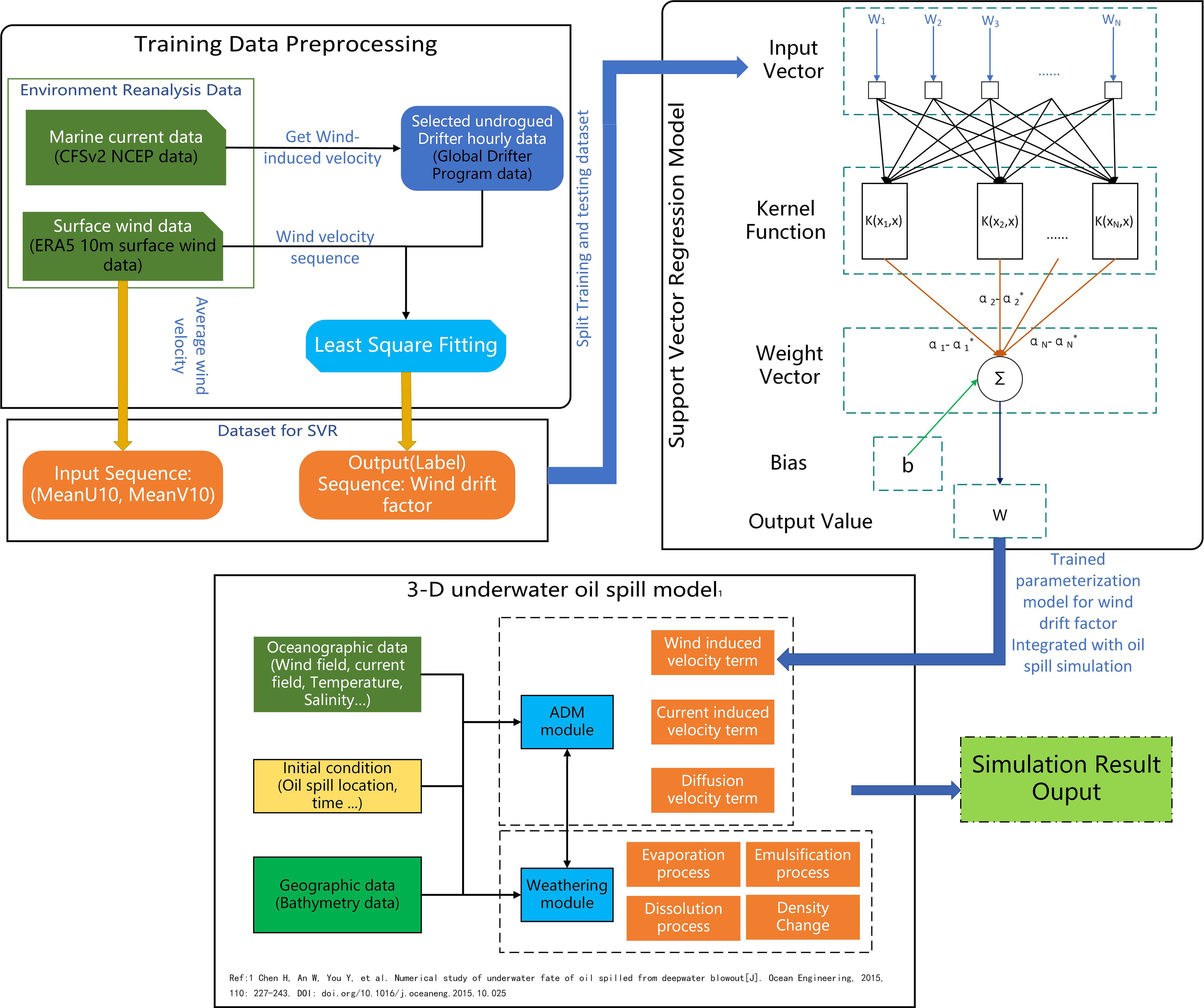
Figure 1 Overall technical route of parameterization modeling.

The whole parameterization modeling consisted of the parts of pre-processing, SVR model, and oil spill simulation model. The basic idea of the model is to integrate the pre-trained SVR-PM into the ADM module of the oil spill simulation. At each time step of oil spill simulation, before calculating the wind-induced speed of oil particles, sea surface wind speed read from background environmental field at this location at this time is input to the SVR-PM, and the WDF corresponding to the current wind speed is obtained in real time and applied to the calculation of wind speed. The details of the SVR-PM are described below.

2.4.1 Preprocessing

Buoy drift at sea results from the combined effects of multiple factors including wind, waves, currents, and turbulence. Nonetheless, in this study, due to their lesser impacts, the influences of waves and turbulence are not considered, focusing instead on wind and current effects on buoys. It is crucial to note that the drift characteristics of buoys and oil particles may differ significantly. The actual drifting process of oil particles is not easily captured, and only the overall drifting and convergence of oil films can be discerned through various observation methods. Consequently, the modeling of the oil spill drift process must rely on other types of drift data. Buoy data, with its large amount, long drift time, and wide spatial and temporal distribution, becomes a preferable choice. It can serve as an approximation of the oil particle transport model.

The entire data preprocessing part consists of the following steps.

2.4.1.1 Filtering undrogued buoy data

This is vital for studying the wind-induced velocity component. For the drifting process of buoys at sea, the primary dynamic elements originate from the currents and sea surface wind. We aim to study the mechanism of wind effect on the buoy, and the role of a drogue is to filter out the wind action and capture the current magnitude. Hence, the initial step of data preprocessing involves selecting undrogued drifter data.

2.4.1.2 Obtaining the buoy’s wind-induced speed

As noted earlier, the buoy’s drift results from the combined effect of wind and currents. The WDF primarily illustrates the relationship between the original wind speed and the wind-induced velocity. Therefore, the wind-induced speed can be attained though this equation:

$\begin{array}{ll}\begin{array}{l}{U}_{ind}=U_{ori}-U_{current}\hfill \\ V_{ind}=V_{ori}-V_{current}\hfill \end{array}& (18)\end{array}$

where $U_{ind} \text{and} V_{ind}$ are the wind-induced velocity of drifters in $U$ and $V$ directions; $U_{ori}\text{ and }{V}_{ori}$ are the original speed of drifters on the sea; $U_{current} \text{and} V_{current}$ are the sea current velocity corresponding to the original speed at each position at each moment.

2.4.1.3 Calculating the drifter’s WDF

Once the sequence of wind-induced velocity and original wind speed has been obtained, the WDF in Eq. 4 can be calculated using following formula:

$\begin{array}{ll}f(W,\alpha ,\beta )=\alpha ·A·W, W=(U_{wind},V_{wind}),A=\left(\begin{array}{cc}cos\beta & sin\beta \\ -sin\beta & cos\beta \end{array}\right)& (19)\end{array}$

$\begin{array}{ll}\text{minimize} {(f(W,\alpha ,\beta )-U)}^2,U=(U_{ind},V_{ind})& (20)\end{array}$

where $U_{wind}\text{ and }{V}_{wind}$ are the sea surface wind speed components in $U$ and $V$ directions, and $U_{ind}\text{ and }{V}_{ind}$ are the wind-induced velocity in U and V directions. Using the least square fitting towards Eq. 20 through inputting a sequence of wind-induced velocity and wind speed can get the value of WDF.

2.4.2 Training and integrating with oil spill model

Since calculating the WDF requires a series of wind speed values and the corresponding wind-induced velocity values to complete the fitting process using mathematical methods, it is impossible to train the SVR model with the wind speed series data as the input and the corresponding WDF as the output of the training set. This is because, in the final oil spill model, the only input that can be provided at each time step for calculating the wind-induced velocity is background environmental field wind velocity at current time step for both U and V values. To resolve this conflict, the series of wind speed values used for the fitting process are averaged to obtain mean wind velocity, denoted as MeanU10 and MeanV10, which represent the average wind speed at a 10-m height above sea level in the U and V directions, respectively, as input data for the training process of the SVR-PM. The corresponding WDF α obtained by least squares fitting serves as the corresponding output (label data). After this preprocessing, one buoy corresponds to one sample containing the average U and V wind speed values, MeanU10 and MeanV 10, and the corresponding WDFs. Numerous buoy sample data are collected and split into training and test datasets for the training and cross-validation process of the SVR model, ultimately yielding the complete SVR-PM.

Upon completing the training, the model is integrated with the ADM module of the oil spill simulation. The SVR-PM accepts the wind velocity as input, then predicts the corresponding WDF value before calculating the wind-induced velocity term at each time step. Finally, the predicted WDF values and the U and V wind speed components are used in Eq. 4 to complete calculation of the wind induced speed term of each oil particle.

3 Experiment

In this section, the details of data used in preprocess part, model training, and oil spill simulation will be introduced. In addition, the configuration of the simulation will be discussed.

3.1 Data preparation

In the preprocessing part, the data to be used include buoy data, sea surface reanalysis wind data, and ocean hydrodynamic data.

3.1.1 Buoy data preprocess

The buoy data are from satellite-tracked surface drifting buoys (drifters) of the NOAA Global Drifter Program. In our study, the velocity and position of buoy were used, which can be found in Elipot et al. (2016, 2022). The processing of raw buoy data unfolds in several stages: outlier processing, selection of undrogued data, temporal segmentation, and wind-induced speed calculation. The raw data selected for this study encompass a total of 4,515 buoys situated within the spatial range of the global oceans spanning the decade from 2010 to 2020. Initially, the raw data are subjected to outlier removal. While all buoys are initially equipped with drogues to record sea surface currents, drogues may be lost due to various reasons. The variable “drogue_lost_date” is recorded in the dataset. Thus, we need to filter the data to include only those buoys that continue to drift for a specific period of time (100 h) after the drogue is lost. The loss of the drogue causes the buoy to drift under the combined influence of wind and current, making it an ideal subject for our experiment. After filtering, 4,176 buoys remain, their drifting periods varying from a few days to several weeks or even years. The next step involves temporal segmentation. As we consider the buoy data to approximate the trajectory of oil particles during the generation of training data, the raw buoy data must initially undergo preprocessing and partitioning into time series of equal length. Given that the initial period of oil spill distribution and behavioral process is of most interest in most oil spill simulations, we select 480 h as the basis for segmentation. By partitioning the data into 480-h segments, the 4,176 datasets are subdivided into a number of fixed-length buoy velocity sequences.

According to the Section 2.4.1, the pre-processing procedure of the subsequent section is completed, and the data are cleaned and aggregated to obtain the wind-induced velocity and original wind speed sequences of the buoys, with a total of 11,135 sample data. Figure 2 shows the starting positions of all drifters. The distribution is very wide, basically covering all the oceans of the world. The broad spatial and temporal distribution of the data is the essence of the parameterization modeling in this study.

FIGURE 2

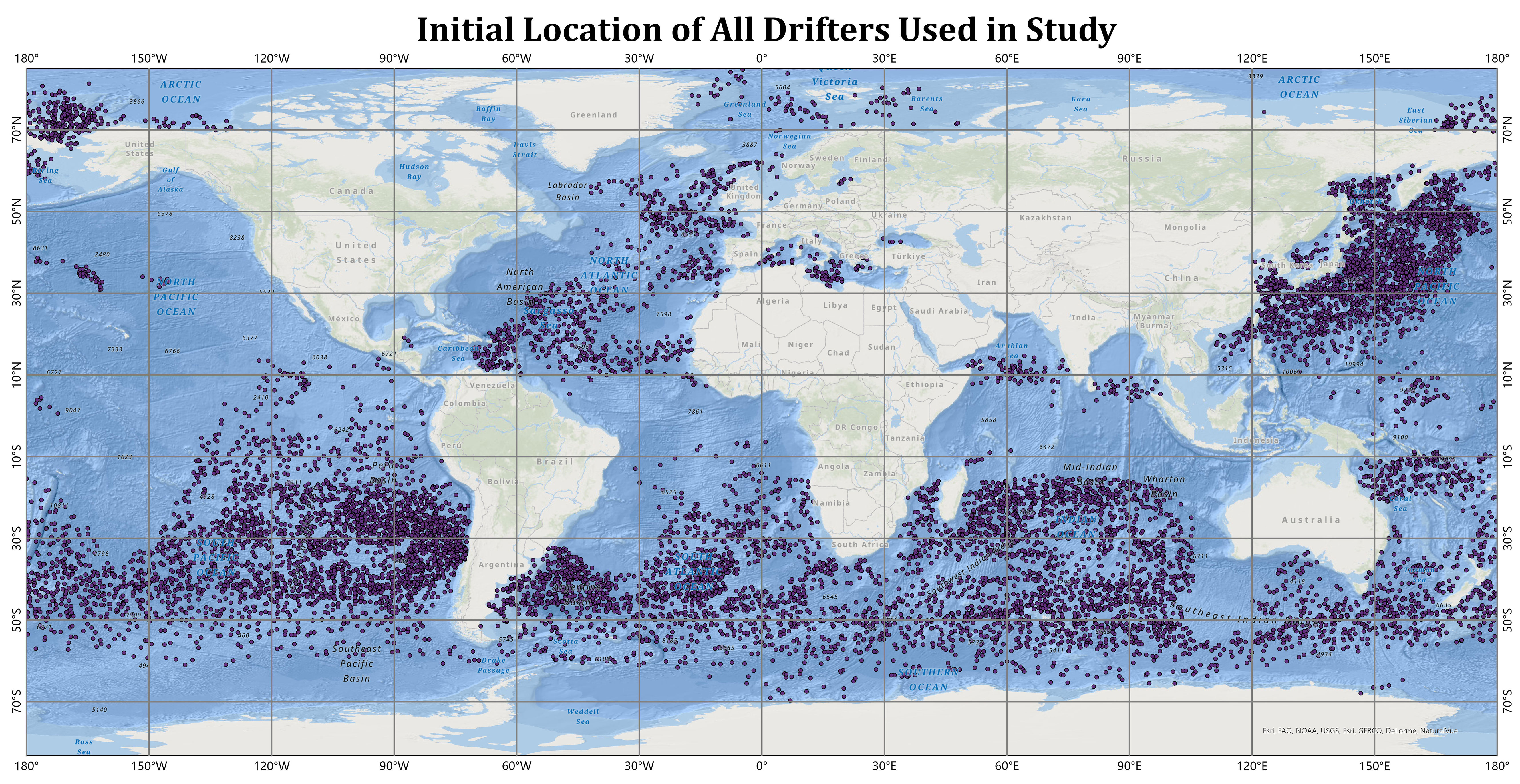
Figure 2 Initial location of all drifters used in this study.

3.1.2 Marine hydrodynamic data

The marine environmental reanalysis data used in this study are divided into two parts: one is the wind and current field data used in combination with buoy data to process and train the SVR-PM; another is the wind, current, and temperature and salt field data used to drive the oil spill simulations. For the segmented buoy data, the environmental field data used to calculate the wind-driven velocity terms and the corresponding WDFs are derived from the ECMWF ERA5 (Hersbach et al., 2023) dataset and the NOAA NCEP (CFSv2) (Saha et al., 2014) dataset. The ERA5 dataset, encompassing hourly data of u and v wind speed variables at 10 m above the sea surface, was utilized. This dataset has a spatial resolution of 0.25° and a spatial and temporal extent that aligns with the range covered by the buoy data, totaling about 750 GB. From the NCEP dataset, we selected hourly data of u and v velocity variables at the sea surface. This dataset has a spatial resolution of 0.5° and a spatiotemporal range consistent with that covered by the buoy data, amounting to approximately 170 GB. After the data processing was completed, bilinear interpolation was used on the wind and current field data to determine the current and wind velocities at each buoy location. The dataset for training the model was obtained by processing according to the scheme outlined in Section 2.4.1.

3.2 Configuration of oil spill model

In order to verify the performance of the SVR-PM, two significant oil spill events in China sea were chosen to make simulation by the proposed model. In addition, satellite remote sensing is a significant method for observing the distribution and fate oil spilled on the sea surface. Several satellite images were obtained to make verification of the proposed model. The details of the configuration and background hydrodynamic data are described in Table 1.

TABLE 1

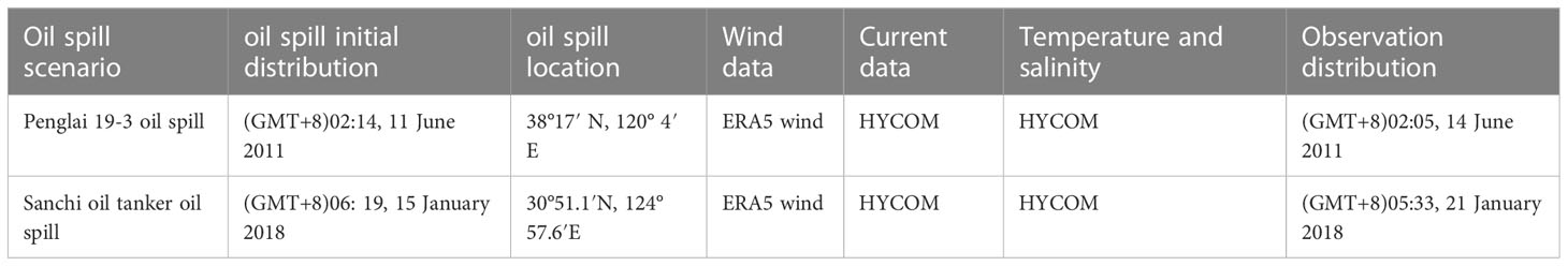
Table 1 Configuration of oil spill scenario.

The wind field data are from the ERA5 wind reanalysis data (Hersbach et al., 2023). In addition, the current, temperature, and salinity data are from HYCOM (https://hycom.org). The dataset used is the output of Global Ocean Forecasting System(GOFS) version 3.1 on the GLBv0.08 grid, which is 0.08° resolution between 40°S and 40°N, poleward of these latitudes. The forecast model run produce the forecast up to 5 days ahead with 3 h frequency, which is stored under GLBv0.08/expt 93.0/uv3z datasets.

Satellite observation is a very essential approach to monitor marine oil spill pollution. There are many types of satellite observations, and the more common means in the marine field is to use SAR satellite observation images to compare with numerical simulation results to verify the accuracy of the model or to study the behavior mechanism of the oil spill (Cheng et al., 2011; Cheng et al., 2014; Xu et al., 2015). On 4 June 2011, oil spill incidents occurred at the Penglai 19-3 oilfield’s Platform B in the Bohai Sea, China, which is operated by the China National Offshore Oil Field, located at 38.3° N, 120.08° E (Xu et al., 2013). These incidents led to the spillage of approximately 700 barrels of oil and 2,500 barrels of mineral oil-based drilling mud onto the seabed. Satellite image observation data from 02:14:57 on 11 June 2011 and 02:05:02 on 14 June 2011 were utilized to validate the model. Used image originated from the Synthetic Aperture Radar (SAR) image from ENVISAT Advanced SAR with wide swath and VV polarization (Xu et al., 2013). A simulation integrating the SVR-PM was conducted from 02:00, 11 June to 02:00, 14 June, lasting 72 h. The primary aim of the proposed modeling focused on the trajectory of surface oil particles affected by wind. The oil slick distribution at 02:00 on 11 June was selected as the initial conditions for the Penglai 19-3 case, and the distribution at 02:00 on 14 June served as the verification distribution, as show in Figure 3.

FIGURE 3

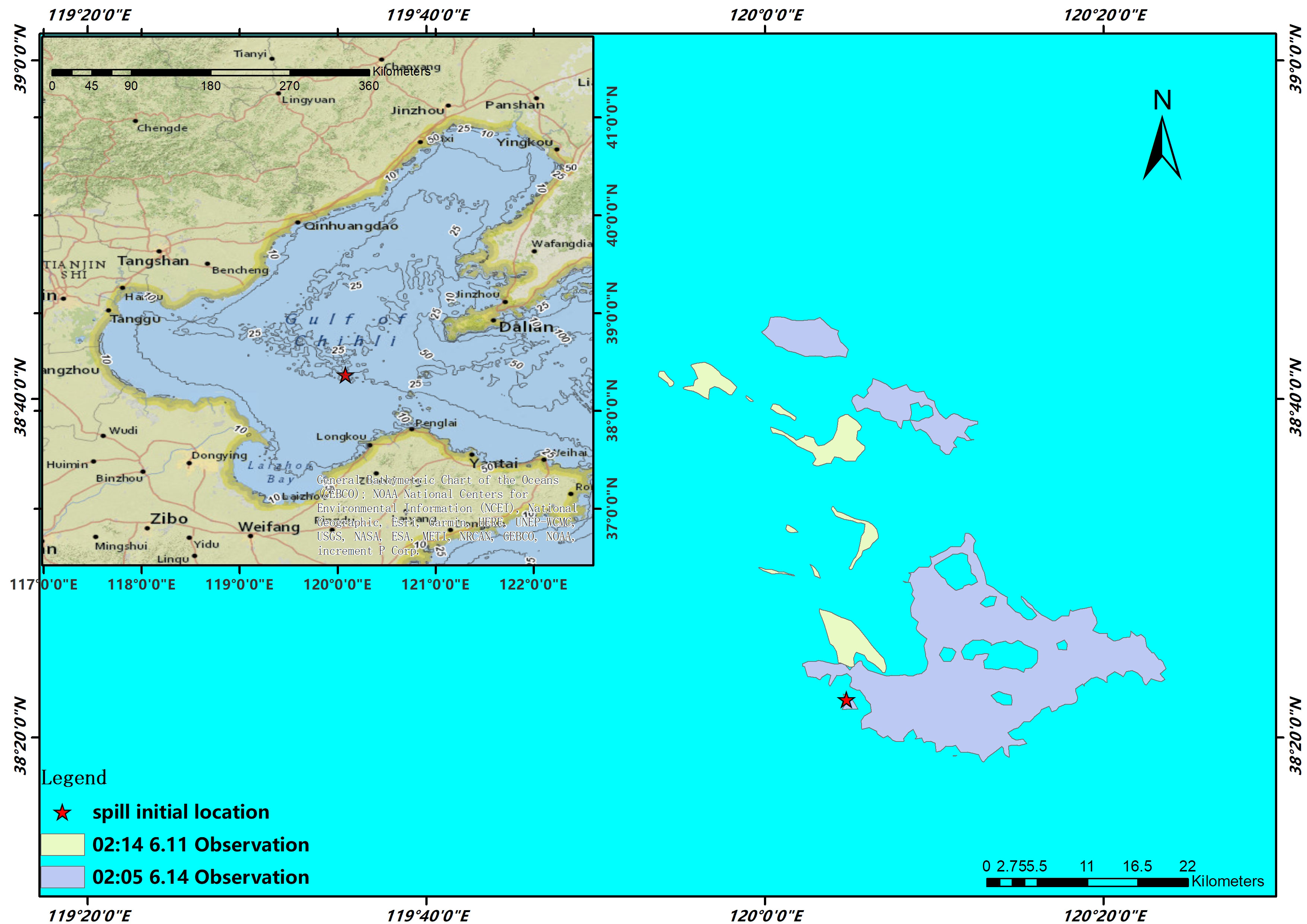
Figure 3 ENVISAT ASAR observation (wide swath and VV polarization) of Penglai 19-3 oil spill in 11.6.2011 and 14.6.2011.

The Panama-registered oil tanker Sanchi (IMO:9356608), en route from Iran to South Korea, collided with the Chinese bulk carrier CF Crystal (IMO:9497050) at 30°51.1′N, 124°57.6′E in the East China Sea at 19:50 on 6 January 2018. The collision resulted in an oil leak, subsequent fire, and explosions. The tanker drifted while burning for approximately 8 days and sank in water 115 m deep at 28°22′N, 125°55′E at 16:45 on 14 January. The flames on the sea surface did not extinguish until 09:58 on 15 January. SAR images by the Chinese Gaofen-3 were also used in this case. The satellite observation at 06:19 on 15 January with 10 m resolution and 100 km swath was used as the initial distribution condition, and the observation at 05:33 on 21 January with 50 m resolution and 300 km swath (Pan et al., 2020) served as the verification distribution, as shown in Figure 4.

FIGURE 4

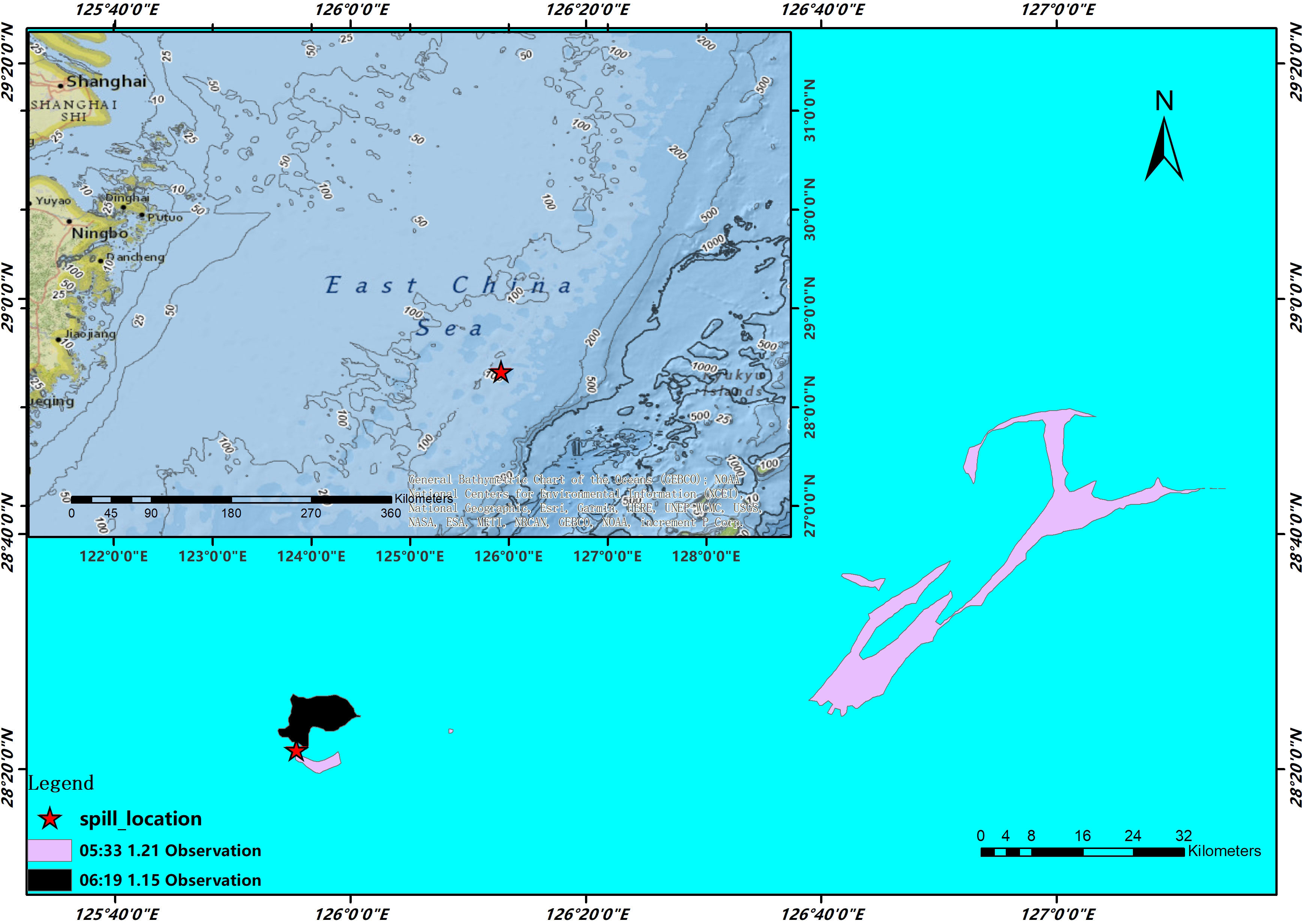
Figure 4 Chinese Gaofen-3 SAR observation of Sanchi oil spill in 1.15 (10 m resolution and 100 km swath) and 1.21 (50 m resolution and 300 km swath), 2018.

4 Results and discussion

This section will validate the accuracy of the proposed model. First, the selection of hyperparameters in the training process of the SVR model will be described. Then, the simulation results of the proposed oil spill model integrated with SVR-PM will be compared with the satellite observation data. Finally, the simulation results of wind drift coefficients derived from the traditional method rate are compared with the experimental results of the proposed model, and final conclusions are drawn. A set of hyperparameter combinations with relatively optimal performance was found by training and model tuning the SVR model using MATLAB regression learning toolbox using 11,135 buoy and wind field data after pre-processing. Kernel function was radial basis function or medium Gaussian function, the kernel scale was 1.4, and the box constraint and epsilon were automatically set, also with standardize training data. Several metrics including root mean square error (RMSE), mean absolute error (MAE), mean square error (MSE), and coefficient of determination ($R^2$) were used to evaluate the performance of SVR model. RMSE was 0.9861, MAE was 0.50958, MSE was 0.0618, and $R^2$ was 0.67.

4.1 Satellite observation verification

The simulation of the Penglai 19-3 oil spill employing the proposed model is depicted in Figure 5. The black area in the figure represents observational data from 11 June, which is utilized as input to simulate the subsequent 72-h behavior using the advection diffusion and weathering modules in the oil spill simulation. The simulation result for 14 June is denoted as the red area in the figure. Although there is less agreement with the observed data (depicted in pink) in the two northern parts, the overall trend is similar. For the larger southern area, the simulated results fall predominantly within the observational data coverage. However, there is a significant discrepancy in the oil slick area. It is important to note that the oil spill model in this study only considers the actions of surface oil particles. As the spill point in this incident was actually below the surface, the model does not account for oil–water interactions within the water column, sunken and submerged oil, or subsequent spills following the initial oil spill. Consequently, the oil slick in the simulation results was considerably smaller than what was observed in reality.

FIGURE 5

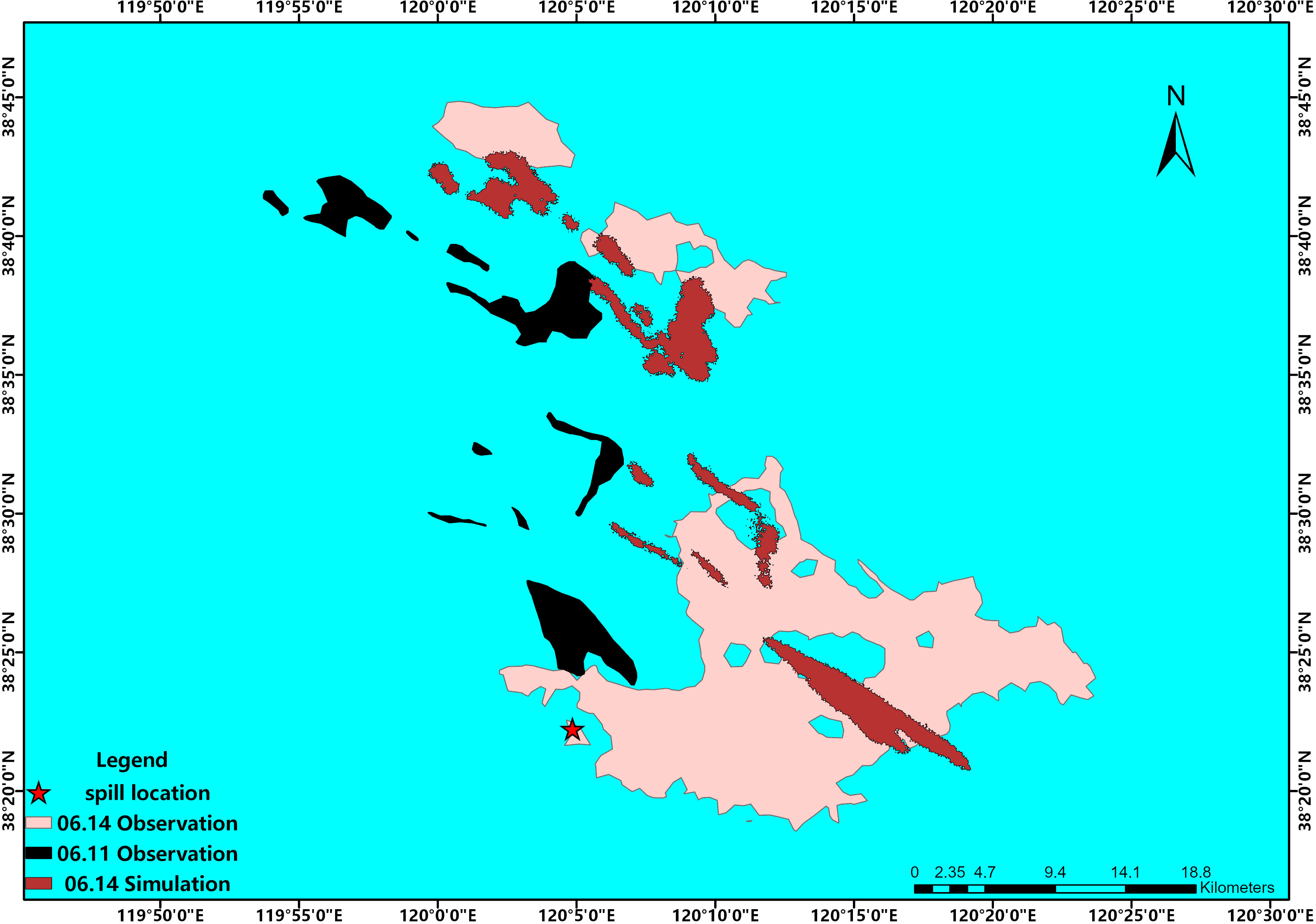
Figure 5 Validation of Penglai 19-3 oil spill range from 11.6.2011 to 14.6.2011.

Figure 6 presents the simulation results of the Sanchi oil spill incident, juxtaposed with satellite observational images. The black portion illustrates observational data from 15 January, which serve as an input for the simulation of the subsequent 144-h behavior. The simulation reveals a commendable agreement between the distribution of the oil slick and the satellite observational data. The only discrepancy lies in the area covered by the oil slick, which is an acceptable margin of error given the reasons previously discussed.

FIGURE 6

Figure 6 Validation of Sanchi oil spill range from 15.1.2018 to 21.1.2018.

4.2 Comparison with traditional method

In the traditional oil spill model, the WDF is set using empirical values. According to the previous section, two values are usually used: one is 0–0.03, and the other is 0–0.06. In this section, the simulation results using empirical values are compared with those using parameterization models to verify the feasibility and accuracy of the parameterization model. In addition, based on Eq. 12 in Guo et al. (2018), an index used to quantitatively evaluate the oil spill simulation results was introduced to measure the accuracy of the model:

$\begin{array}{ll}{P}_{cov}=0.5*\frac{A_{so}}{A_O}+0.5*\frac{A_{so}}{A_S}& (21)\end{array}$

where $P_{cov}$ is the coverage percent of oil spill simulation; the closer it is to 1, the more accurate the simulation is. $A_{so}$ is the superposition of the observed and simulated areas. $A_S$ is the areas of the simulation. $A_O$ is the observed areas.

Figures 7 and 8 present the simulation results when the WDF is set to 0.03 and 0.05, respectively. In addition, these three schemes are denoted as Experiment 1 (Exp. 1) and Exp. 2. The $P_{cov}$ and areas were calculated through the spatial analysis toolbox in ArcGIS. The comparison results are detailed in Table 2. Looking at the Penglai 19-3 case, the simulation shows a substantial deviation when the WDF is set at 0.03, a value typically used in most traditional oil spill models. Regarding $P_{cov}$, the SVR-PM’s $P_{cov}$ reaches approximately 19%. On the contrary, in Exp. 1, there is no overlap between the simulation result and observed data, yielding a $P_{cov}$ of 0.

FIGURE 7

Figure 7 Comparison between the parameterization model and WDF set as 0.03 for two oil spill cases.

FIGURE 8

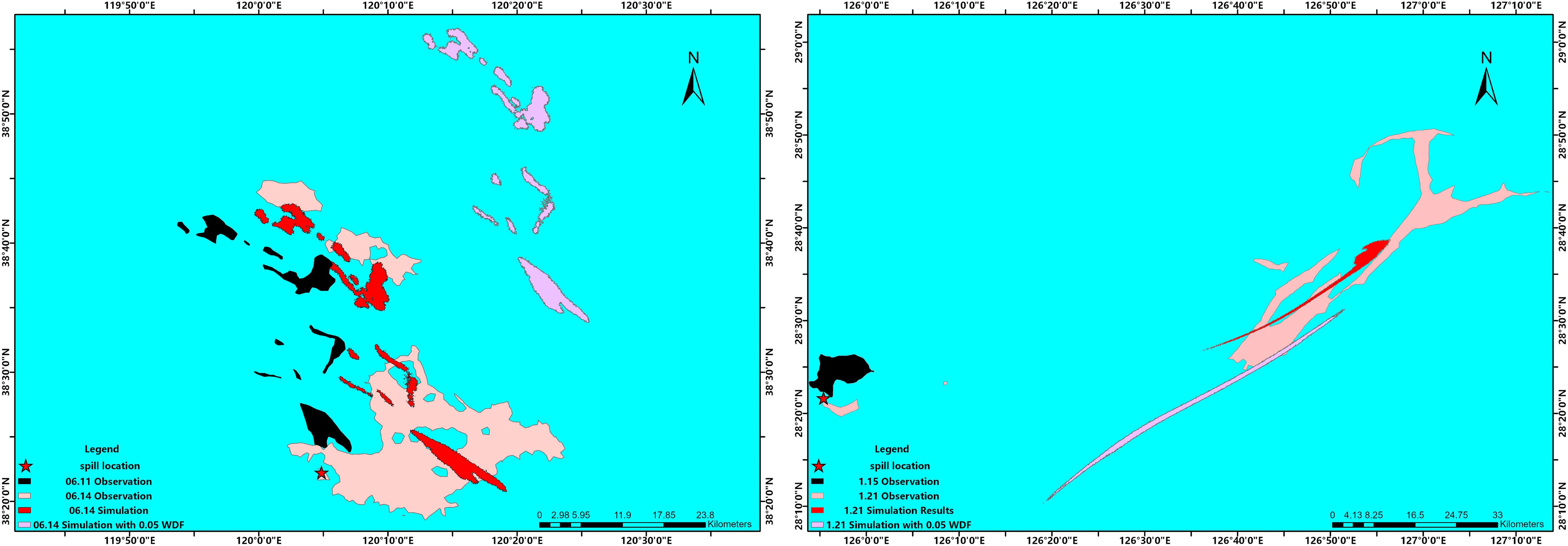
Figure 8 Comparison between the parameterization model and WDF set as 0.05 for two oil spill cases.

TABLE 2

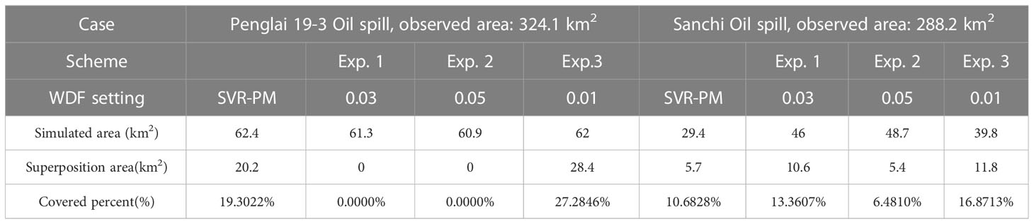
Table 2 Accuracy evaluation between SVR-PM and constant WDF settings.

As for the Sanchi case, the area covered by the simulation is marginally larger than that obtained using the proposed SVR-PM model. The superposition area of the SVR-PM in the Sanchi case is approximately $5.7 {\text{km}}^2$, while it is approximately $10.6 {\text{km}}^2$ in Exp. 1. Despite the superposition area in Exp. 1 being roughly double than that of SVR-PM, the $P_{cov}$ values between them are closely comparable. This minor difference in accuracy, coupled with the area in the southeast corner slightly exceeding the observed data, poses a challenge.

Based on the works of (Reed et al., 1994; Carson et al., 2013), the WDF is typically set below 6%, leading us to conduct Exp.2. However, the resulting effects of both cases showed a significant divergence, making the outcomes less acceptable. Specifically, the $P_{cov}$ of both cases proved to be less accurate than the results obtained from the SVR-PM. This highlights the importance of the precise setting of WDF and the potential of SVR-PM to enhance the accuracy of oil spill simulations.

In our final experiment (denoted as Exp. 3), we set the WDF to 0.01, as demonstrated in Figure 9. The results revealed a marked improvement in model performance compared to both Exp. 1 and Exp. 2. For the Penglai 19-3 case, the coverage percentage ($P_{cov}$) is almost 10% higher than the results of SVR-PM, and the area of overlap in Exp. 3 is approximately 50% larger. Concerning the Sanchi case, the coverage area of Exp. 3 is twice as large as that of SVR-PM, with a discrepancy in $P_{cov}$ of nearly 7%. This may suggest that setting the WDF to 0.01 results in higher accuracy in oil spill simulations for the two cases considered in this study compared to the proposed model. However, it is critical to note that determining the appropriate WDF for any oil spill simulation remains an open problem that must be addressed before the first simulation is conducted. Several sensitivity experiments are required to fine tune the WDF to accurately simulate the behavior of oil particles on the sea surface. In the context of the experiments carried out in this study, at least two or more trials are necessary to find an optimal setting, underscoring the advantage of the model proposed in this paper.

FIGURE 9

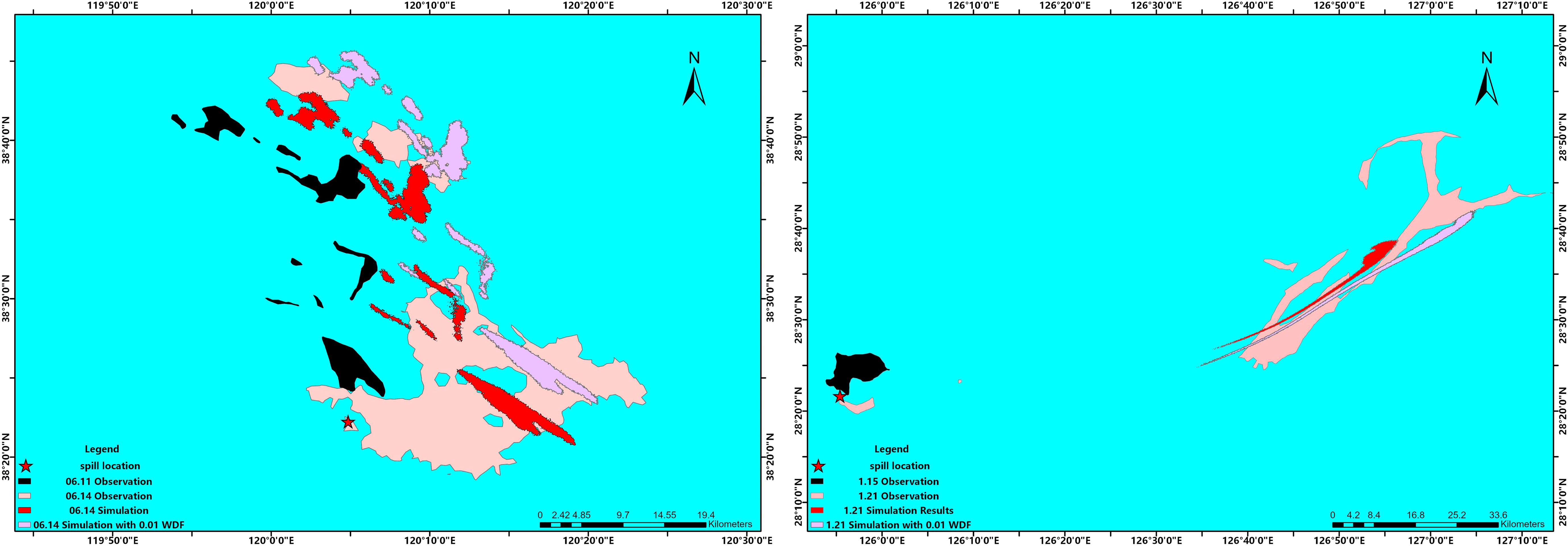
Figure 9 Comparison between the parameterization model and WDF set as 0.01 for two oil spill cases.

Considering the combined results among simulations, the parameterization model proposed in this study demonstrates satisfactory performance across varying oil spill simulation scenarios. For Penglai 19-3 case, the average $P_{cov}$ of three experiments is approximately 13%, but the coverage percentage of SVR-PM is better than this, which could reach 19%. Similarly, in the Sanchi case, the $P_{cov}$ of SVR-PM can also reach the mean of three experiments. Given the time differences between the two incidents and the geographical variances, the role of the wind on sea-surface oil particles proves to be highly significant. The simulation results validate the utility of the WDF parameterization scheme in the oil spill model, utilizing numerous buoy data with extensive spatial and temporal distribution. The broad temporal range ensures the accommodation of wind effect variations across different seasons. Moreover, the extensive spatial distribution endows the model with some degree of geographical generalization capability.

5 Conclusion and prospect

In this study, we propose an SVR-based parameterization modeling method, termed SVR-PM, to parameterize the WDF in oil spill simulations. Most existing oil spill simulations typically use a fixed empirical value for the WDF. However, this approach has several limitations as the WDF determines the proportion of wind action influencing the motion of oil particles. To address these limitations, we utilize SVR, a machine learning algorithm widely used for regression problems, to construct a parameterization model of the WDF. The training data for this model comprise an extensive set of buoy data, which is temporally and spatially distributed, coupled with corresponding ocean hydrodynamic reanalysis data. Using these resources, we train an SVR prediction model that can accept real-time wind speed inputs and provide the WDF under corresponding wind speed conditions. We then integrate this model into an oil spill simulation that considers the convective diffusion of surface oil particles and the weathering process, transforming the WDF from a constant to a dependent variable that varies with wind speed.

During the validation phase, we use satellite observations of two high-impact oil spills that occurred offshore China to verify the model’s accuracy. Although the fit of the SVR model is approximately 70%, it still delivers better results than traditional methods when used in oil spill event simulations. Furthermore, the model can achieve accurate results without adjusting parameters and settings for oil spill simulations across various geographical locations and time periods (seasons). The $P_{cov}$, which measure the accuracy of oil spill simulation, could reach the average level of simulation results of different schemes of WDF settings. The SVR-PM’s advantage lies in enhancing the accuracy of oil spill simulations and demonstrating strong adaptability and generalizability over time and space. This advancement holds significant implications for maritime departments and emergency disaster response units.

While this study presents promising findings, there are still a few limitations worth noting:

1. The parameterization modeling in the current research does not take into consideration the $\beta$-values. The wind drift effect is, in reality, determined by both the wind drift factor $\alpha$ and the wind deflection angle $\beta$. However, this paper only considers the parameterization of $\alpha$ and does not investigate the magnitude of the wind drift angle, $\beta$. Future studies should give more attention to the wind drift angle.

2. This study only selected one type of buoy data to investigate its wind drift mechanism. Nonetheless, the nature of passive drift at sea can vary based on different types of buoys, considering differences in size and submergence depths. Additionally, there are numerous factors influencing the effects of various ocean dynamics elements (e.g., wind, waves, turbulence) on drifting objects. These influencing factors ought to be considered in future research.

3. Other coefficients or stochastic processes that determine the behavior and fate of the oil spill still need to be addressed. For example, the random walk method, commonly used in modeling the spread of oil spills, involves key parameters that should be considered for modeling in future studies of such processes.

Data availability statement

The raw data supporting the conclusions of this article will be made available by the authors, without undue reservation.

Author contributions

DL: methodology, coding, and original draft preparation. YL: supervision and reviewing. LM: conceptualization and reviewing. All authors contributed to the article and approved the submitted version.

Funding

This work was supported by the National Natural Science Foundation of China (grant number U2006210), Shenzhen Science and Technology Program (grant number JSGG20210713091538011), and Shenzhen Science and Technology Program (grant number KCXFZ20211020164015024).

Conflict of interest

The authors declare that the research was conducted in the absence of any commercial or financial relationships that could be construed as a potential conflict of interest.

Publisher’s note

All claims expressed in this article are solely those of the authors and do not necessarily represent those of their affiliated organizations, or those of the publisher, the editors and the reviewers. Any product that may be evaluated in this article, or claim that may be made by its manufacturer, is not guaranteed or endorsed by the publisher.

References

Al-Rabeh A. H., Cekirge H. M., Gunay N. (1989). A stochastic simulation model of oil spill fate and transport. Appl. Math. Model. 13, 322–329. doi: 10.1016/0307-904X(89)90134-0

CrossRef Full Text | Google Scholar

Al-Rabeh A. H., Lardner R. W., Gunay N. (2000). Gulfspill version 2.0: a software package for oil spills in the arabian gulf. Environ. Model. Soft. 15, 425–442. doi: 10.1016/S1364-8152(00)00013-X

CrossRef Full Text | Google Scholar

ASCE (1996). State-of-the-art review of modeling transport and fate of oil spills. J. Hydraulic Eng. 122, 594–609. doi: 10.1061/(ASCE)0733-9429(1996)122:11(594

CrossRef Full Text | Google Scholar

Bozkurtoğlu Ş.N.E. (2017). Modeling oil spill trajectory in bosphorus for contingency planning. Mar. Pollut. Bull. 123, 57–72. doi: 10.1016/j.marpolbul.2017.09.029

PubMed Abstract | CrossRef Full Text | Google Scholar

Cao R., Chen H., Rong Z., Lv X. (2021). Impact of ocean waves on transport of underwater spilled oil in the bohai sea. Mar. Pollut. Bull. 171, 112702. doi: 10.1016/j.marpolbul.2021.112702

PubMed Abstract | CrossRef Full Text | Google Scholar

Carson H. S., Lamson M. R., Nakashima D., Toloumu D., Hafner J., Maximenko N., et al. (2013). Tracking the sources and sinks of local marine debris in hawaii. Mar. Environ. Res. 84, 76–83. doi: 10.1016/j.marenvres.2012.12.002

PubMed Abstract | CrossRef Full Text | Google Scholar

Casdagli M. (1989). Nonlinear prediction of chaotic time series. physica d. Nonlinear Phenomena 35, 335–356. doi: 10.1016/0167-2789(89)90074-2

CrossRef Full Text | Google Scholar

Chen H., An W., You Y., Lei F., Zhao Y., Li J. (2015). Numerical study of underwater fate of oil spilled from deepwater blowout. Ocean Eng. 110, 227–243. doi: 10.1016/j.oceaneng.2015.10.025

CrossRef Full Text | Google Scholar

Chen H.-z., Li D.-m., Li X. (2007). Mathematical modeling of oil spill on the Sea and application of the modeling in daya bay. J. Hydrodynam. 19, 282–291. doi: 10.1016/S1001-6058(07)60060-2

CrossRef Full Text | Google Scholar

Chen S., Wang W., van Zuylen H. (2009). Construct support vector machine ensemble to detect traffic incident. Expert Syst. Appl. 36, 10976–10986. doi: 10.1016/j.eswa.2009.02.039

CrossRef Full Text | Google Scholar

Chen C., Zhang G., Qian Z., Tarefder R. A., Tian Z. (2016). Investigating driver injury severity patterns in rollover crashes using support vector machine models. Accident Anal. Prev. 90, 128–139. doi: 10.1016/j.aap.2016.02.011

CrossRef Full Text | Google Scholar

Cheng Y., Li X., Xu Q., Garcia-Pineda O., Andersen O. B., Pichel W. G. (2011). SAR observation and model tracking of an oil spill event in coastal waters. Mar. Pollut. Bull. 62, 350–363. doi: 10.1016/j.marpolbul.2010.10.005

PubMed Abstract | CrossRef Full Text | Google Scholar

Cheng Y., Liu B., Li X., Nunziata F., Xu Q., Ding X., et al. (2014). Monitoring of oil spill trajectories with COSMO-SkyMed X-band SAR images and model simulation. IEEE J. Selected Topics Appl. Earth Observat. Remote Sens. 7, 2895–2901. doi: 10.1109/JSTARS.2014.2341574

CrossRef Full Text | Google Scholar

De Dominicis M., Pinardi N., Zodiatis G., Archetti R. (2013a). Medslik-ii, a lagrangian marine surface oil spill model for short-term forecasting - part 2: numerical simulations and validations. Geoscientific Model. Dev. 6, 1871–1888. doi: 10.5194/gmd-6-1871-2013

CrossRef Full Text | Google Scholar

De Dominicis M., Pinardi N., Zodiatis G., Lardner R. (2013b). Medslik-ii, a lagrangian marine surface oil spill model for short-term forecasting - part 1: theory. Geoscientific Model. Dev. 6, 1851–1869. doi: 10.5194/gmd-6-1851-2013

CrossRef Full Text | Google Scholar

Deng Z., Yu T., Jiang X., Shi S., Jin J., Kang L., et al. (2013). Bohai sea oil spill model: a numerical case study. Mar. Geophys. Res. 34, 115–125. doi: 10.1007/s11001-013-9180-x

CrossRef Full Text | Google Scholar

Dominicis M. D., Bruciaferri D., Gerin R., Pinardi N., Poulain P. M., Garreau P., et al. (2016). A multi-model assessment of the impact of currents, waves and wind in modelling surface drifters and oil spill. Deep Sea Res. Part II: Top. Stud. Oceanog. 133, 21–38. doi: 10.1016/j.dsr2.2016.04.002

CrossRef Full Text | Google Scholar

Elipot S., Lumpkin R., Perez R. C., Lilly J. M., Early J. J., Sykulski A. M. (2016). A global surface drifter data set at hourly resolution. J. Geophys. Res.: Oceans 121, 2937–2966. doi: 10.1002/2016JC011716

CrossRef Full Text | Google Scholar

Elipot S., Syskulsksi A., Lumpkin R., Centurioni L., Pazos M. (2022). Hourly location, current velocity, and temperature collected from global drifter program drifters world-wide. doi: 10.25921/x46c-3620

PubMed Abstract | CrossRef Full Text | Google Scholar

Elliott A. J. (1986). Shear diffusion and the spread of oil in the surface layers of the north sea. Deutsche Hydrografische Z. 39, 113–137. doi: 10.1007/BF02408134

CrossRef Full Text | Google Scholar

Fay J. A. (1971). Physical processes in the spread of oil on a water surface. Int. Oil Spill Conf. Proc. 1971, 463–467. doi: 10.7901/2169-3358-1971-1-463

CrossRef Full Text | Google Scholar

French-McCay D. P. (2004). Oil spill impact modeling: development and validation. Environ. Toxicol. Chem. 23, 2441–2456. doi: 10.1897/03-382

PubMed Abstract | CrossRef Full Text | Google Scholar

Guo W., Hao Y., Zhang L., Xu T., Ren X., Cao F., et al. (2014). Development and application of an oil spill model with wave-current interactions in coastal areas. Mar. Pollut. Bull. 84, 213–224. doi: 10.1016/j.marpolbul.2014.05.009

PubMed Abstract | CrossRef Full Text | Google Scholar

Guo W., Jiang M., Li X., Ren B. (2018). Using a genetic algorithm to improve oil spill prediction. Mar. Pollut. Bull. 135, 386–396. doi: 10.1016/j.marpolbul.2018.07.026

PubMed Abstract | CrossRef Full Text | Google Scholar

Guo W., Wu G., Jiang M., Xu T., Yang Z., Xie M., et al. (2016). A modified probabilistic oil spill model and its application to the dalian new port accident. Ocean Eng. 121, 291–300. doi: 10.1016/j.oceaneng.2016.05.054

CrossRef Full Text | Google Scholar

Hearst M., Dumais S., Osuna E., Platt J., Scholkopf B. (1998). Support vector machines. IEEE Intelligent Syst. their Appl. 13, 18–28. doi: 10.1109/5254.708428

CrossRef Full Text | Google Scholar

Hersbach H., Bell B., Berrisford P., Biavati G., Horányi A., Muñoz Sabater J., et al. (2023). ERA5 hourly data on single levels from 1940 to present. doi: 10.24381/cds.adbb2d47

CrossRef Full Text | Google Scholar

Johansen O. (1982). Dispersion of oil from drifting slicks. Spill Technol. Newslett. 134, 370. Available at: https://scholar.google.com/scholar?cluster=10880298167213677474&hl=en&as_sdt=2005&sciodt=0,5&scioq=Johansen,+O.+(1982).+Dispersion+of+oil+from+drifting+slicks.+Spill+Technol.+Newslett.+134,+370.

Google Scholar

Kim T.-H., Yang C.-S., Oh J.-H., Ouchi K. (2014). Analysis of the contribution of wind drift factor to oil slick movement under strong tidal condition: hebei spirit oil spill case. PloS One 9, 1–14. doi: 10.1371/journal.pone.0087393

CrossRef Full Text | Google Scholar

Lau K. W., Wu Q. H. (2008). Local prediction of non-linear time series using support vector regression. Pattern Recognition 41, 1539–1547. doi: 10.1016/j.patcog.2007.08.013

CrossRef Full Text | Google Scholar

Lehr W., Jones R., Evans M., Simecek-Beatty D., Overstreet R. (2002). Revisions of the adios oil spill model. Environ. Model. Soft. 17, 189–197. doi: 10.1016/S1364-8152(01)00064-0

CrossRef Full Text | Google Scholar

Li Y., Chen H., Lv X. (2018). Impact of error in ocean dynamical background, on the transport of underwater spilled oil. Ocean Model. 132, 30–45. doi: 10.1016/j.ocemod.2018.10.003

CrossRef Full Text | Google Scholar

Li Z., Liu P., Wang W., Xu C. (2012). Using support vector machine models for crash injury severity analysis. Accident Anal. Prev. 45, 478–486. doi: 10.1016/j.aap.2011.08.016

CrossRef Full Text | Google Scholar

Liu Z., Chen Q., Zhang Y., Zheng C., Cai B., Liu Y. (2022). Research on transport and weathering of oil spills in jiaozhou bight, china. Regional Stud. Mar. Sci. 51, 102197. doi: 10.1016/j.rsma.2022.102197

CrossRef Full Text | Google Scholar

Marques W. C., Stringari C. E., Kirinus E. P., Möller O. O., Toldo E. E., Andrade M. M. (2017). Numerical modeling of the tramandaí beach oil spill, Brazil–case study for January 2012 event. Appl. Ocean Res. 65, 178–191. doi: 10.1016/j.apor.2017.04.007

CrossRef Full Text | Google Scholar

Mohan R., Kankara R., Venkatachalapathy R. (2014). “Oil spill trajectory modelling of chennai coast, east coast of india,” in Proceedings of 5th Indian National Conference on Harbour and Ocean Engineering (INCHOE2014), (Goa, India), Vol. 5–7.

Google Scholar

Pan Q., Yu H., Daling P. S., Zhang Y., Reed M., Wang Z., et al. (2020). Fate and behavior of sanchi oil spill transported by the kuroshio during january -february 2018. Mar. Pollut. Bull. 152, 110917. doi: 10.1016/j.marpolbul.2020.110917

PubMed Abstract | CrossRef Full Text | Google Scholar

Pan Q., Zhu X., Wan L., Li Y., Kuang X., Liu J., et al. (2021). Operational forecasting for sanchi oil spill. Appl. Ocean Res. 108, 102548. doi: 10.1016/j.apor.2021.102548

CrossRef Full Text | Google Scholar

Reed M., Johansen Ø., Brandvik P. J., Daling P., Lewis A., Fiocco R., et al. (1999). Oil spill modeling towards the close of the 20th century: overview of the state of the art. Spill Sci. Technol. Bull. 5, 3–16. doi: 10.1016/S1353-2561(98)00029-2

CrossRef Full Text | Google Scholar

Reed M., Turner C., Odulo A. (1994). The role of wind and emulsification in modelling oil spill and surface drifter trajectories. Spill Sci. Technol. Bull. 1, 143–157. doi: 10.1016/1353-2561(94)90022-1

CrossRef Full Text | Google Scholar

Saha S., Moorthi S., Wu X., Wang J., Nadiga S., Tripp P., et al. (2014). The ncep climate forecast system version 2. J. Climate 27, 2185–2208. doi: 10.1175/JCLI-D-12-00823.1

CrossRef Full Text | Google Scholar

Smola A. J., Schölkopf B. (2004). A tutorial on support vector regression. Stat Comput. 14, 199–222. doi: 10.1023/B:STCO.0000035301.49549.88

CrossRef Full Text | Google Scholar

Spaulding M. L. (1988). A state-of-the-art review of oil spill trajectory and fate modeling. Oil Chem. Pollut. 4, 39–55. doi: 10.1016/S0269-8579(88)80009-1

CrossRef Full Text | Google Scholar

Spaulding M. L. (2017). State of the art review and future directions in oil spill modeling. Mar. Pollut. Bull. 115, 7–19. doi: 10.1016/j.marpolbul.2017.01.001

PubMed Abstract | CrossRef Full Text | Google Scholar

Stolzenbach K. D., Madsen O. S., Adams E. E., Pollack A. M., Copper C. K. (1977). Review and evaluation of basic techniques for predicting the behavior of surface oil slicks (United States: Massachusetts Institute of Technology, Cambridge, MA).

Google Scholar

Tamura H., Miyazawa Y., Oey L.-Y. (2012). The stokes drift and wave induced-mass flux in the north pacific. J. Geophys. Res.: Oceans 117 (C08021). doi: 10.1029/2012JC008113

CrossRef Full Text | Google Scholar

Tu H., Wang X., Mu L., Xia K. (2021). Predicting drift characteristics of persons-in-the-water in the south china sea. Ocean Eng. 242, 110134. doi: 10.1016/j.oceaneng.2021.110134

CrossRef Full Text | Google Scholar

Vapnik V. (1999). The nature of statistical learning theory (New York, USA: Springer science & business media). doi: 10.1007/978-1-4757-3264-1

CrossRef Full Text | Google Scholar

Wang D., Luo Z., Mu L. (2022). Numerical study on the influence of model uncertainties on the transport of underwater spilled oil. Int. J. Environ. Res. Public Health 19, 9274. doi: 10.3390/ijerph19159274

PubMed Abstract | CrossRef Full Text | Google Scholar

Wang J., Shen Y. (2010a). Development of an integrated model system to simulate transport and fate of oil spills in seas. Sci. China Technol. Sci. 53, 2423–2434. doi: 10.1007/s11431-010-4059-4

CrossRef Full Text | Google Scholar

Wang J., Shen Y. (2010b). Modeling oil spills transportation in seas based on unstructured grid, finite-volume, wave-ocean model. Ocean Model. 35, 332–344. doi: 10.1016/j.ocemod.2010.09.005

CrossRef Full Text | Google Scholar

Wang S., Shen Y., Guo Y., Tang J. (2008). Three-dimensional numerical simulation for transport of oil spills in seas. Ocean Eng. 35, 503–510. doi: 10.1016/j.oceaneng.2007.12.001

CrossRef Full Text | Google Scholar

Xu Q., Cheng Y., Liu B., Wei Y. (2015). Modeling of oil spill beaching along the coast of the bohai Sea, China. Front. Earth Sci. 9, 637–641. doi: 10.1007/s11707-015-0515-6

CrossRef Full Text | Google Scholar

Xu Q., Li X., Wei Y., Tang Z., Cheng Y., Pichel W. G. (2013). Satellite observations and modeling of oil spill trajectories in the bohai sea. Mar. Pollut. Bull. 71, 107–116. doi: 10.1016/j.marpolbul.2013.03.028

PubMed Abstract | CrossRef Full Text | Google Scholar

Yapa P. D., Wimalaratne M. R., Dissanayake A. L., DeGraff J. A. (2012). How does oil and gas behave when released in deepwater? J. Hydro-environment Res. 6, 275–285. doi: 10.1016/j.jher.2012.05.002

CrossRef Full Text | Google Scholar

Yapa P. D., Zheng L., Nakata K. (1999). Modeling underwater oil/gas jets and plumes. J. Hydraulic Eng. 125, 481–491. doi: 10.1061/(ASCE)0733-9429(1999)125:5(481

CrossRef Full Text | Google Scholar

Zhu K., Mu L., Tu H. (2019). Exploration of the wind-induced drift characteristics of typical chinese offshore fishing vessels. Appl. Ocean Res. 92, 101916. doi: 10.1016/j.apor.2019.101916

CrossRef Full Text | Google Scholar