Research on the carbon emissions traceability inventory and multi-horizon prediction of ship carbon emissions: a case study of Tianjin Port

Introduction: In recent years, the adverse effects of escalating maritime trade and international shipping– particularly in regard to increased greenhouse gas emissions and their impact on human health– have come to the fore. These issues have thus instigated a surge in pressure to enhance the regulation of shipborne carbon emissions.

Methods: The study utilized the automatic identification system (AIS) data, Lloyd’s register data, and pollutant emission parameters to calculate the carbon emissions from the main engine, auxiliary engine, and boiler of vessels under varying sailing conditions, utilizing the dynamic method of ships. In relation to geographic information and ship trajectory, a comprehensive inventory of ship carbon emissions was developed, revealing pronounced spatiotemporal characteristics. To assure the accuracy of the substantial AIS dataset, procedures including data cleaning, trajectory integration, data fusion, and completion were executed. Such processes are indispensable, given the potential for transmission and storage errors associated with AIS data. To forecast CO₂ emissions over diverse time intervals, a temporal fusion transformer model equipped with attention mechanisms was employed.

Result: The paper furnishes a case study on Tianjin Port, wherein a high-resolution carbon emissions inventory was devised based on AIS data acquired from vessels. This inventory was subsequently employed to generate multi-feature predictions of future carbon emissions. Given the optimal parameter configuration, the proposed method attained P₅₀ and P₉₀ values of 0.244 and 0.118 respectively, thereby demonstrating its efficacy.

Discussion: Recognizing the sources of ship carbon emissions in this region and forecasting such emissions in the future substantiates that this method accurately portrays the laws of ship carbon emissions. Our study provides a scientific basis for decision-making in port and pollution management, enabling the creation of targeted emission reduction policies for ships.

1 Introduction

The shipping industry is becoming increasingly important in international trade as the global economy rapidly develops. Sea transport is the most economical and environmentally friendly way of transporting goods compared to road, rail, and air transport (Shu et al., 2022). The shipping industry is responsible for about 90% of global trade transportation by volume. The industry is fundamental to national economic development and a pillar of national security and national economy (Zhou and Leng, 2021). The number of ships in the industry has grown recently, and their greenhouse gas emissions have increased significantly. If greenhouse gas emissions persist at or surpass the current rate, it will precipitate additional global warming and instigate numerous alterations in the global climate system. Climate change might lead to irreversible effects. For instance, an augmented concentration of CO₂ in the atmosphere may further acidify the environment, thereby negatively affecting marine life. According to the Intergovernmental Panel on Climate Change (IPCC, 2007), if the elevation in the global average warming surpasses 1.5–2.5°C (relative to the period of 1980–1999), an estimated 20–30% of assessed species could face an augmented risk of extinction. The global water-carbon cycle is influenced by climatic conditions (Yin et al., 2023). Climate change hampers the absorption of CO₂ by terrestrial and oceanic entities, resulting in an increase in anthropogenic emissions that remain in the atmosphere. Both the transportation of polluted air from land to sea during monsoon seasons and human activities in the marine environment contribute to air pollution. This leads to atmospheric subsidence and subsequent pollution of the marine environment (Pan et al., 2022).Additionally, atmospheric conditions significantly affect extreme weather events, which subsequently escalate the risk of certain human diseases (Yin et al., 2022). Pressure to prevent and control air pollution has also increased due to its negative impact on the marine environment and its deleterious effects on human health (Zhou and Leng, 2021).

According to the Third IMO Greenhouse Gas Study 2014 released by the International Maritime Organization, carbon emissions from international shipping activities in 2012 were 796 million tonnes in 2012, accounting for 2.2% of total global carbon emissions. However, if no effective measures are taken to reduce emissions, the projected future development of the global economy and energy use based on current development patterns indicates that total CO₂ emissions from the shipping industry will increase by 50%–250% by 2050 (Ouyang et al., 2015). China is the second largest shipowner country in the world (International Ship Network, 2021) and therefore is very influential in decarbonizing the shipping industry. Carbon peak and carbon neutrality were written into The Government Work Report for the first time in early 2021 (The Central People’s Government of the People’s Republic of China, 2021). China is currently in the key stage of the 14th Five-Year Plan, which is also a key window period for realizing the double carbon goal. Effectively managing carbon emissions represents a formidable challenge confronting numerous industries–including the shipping industry–in their pursuit of sustainable development. Indeed, it has evolved into a pivotal and interdisciplinary research subject, eliciting interest from various academic disciplines.

Research in China has shown that pollutants emitted within 12 nautical miles of the coastline account for about 40% of all ship emissions off the coast of China. When the range is increased to 100 nautical miles, the emission of ship pollutants doubles. Ports are intersections of water and road transport networks and are nodes of the maritime network (Chen et al., 2022). Emissions from ships in a port account for about a quarter of total emissions within 200 nautical miles of a port, and nearly 80% of emissions are concentrated at the top 10 busiest ports in China (Li et al., 2018). Prosperous international trade has led to the gradual expansion of large-scale shipping, which has inevitably increased the negative environmental effects of ship emissions. Ship emissions easily diffuse from sea to land under the influence of sea breezes, resulting in urban environmental pollution (Liu et al., 2017). Port areas with heavy vessel traffic decrease air quality in port areas (Ng et al., 2013; Li et al., 2016; Weng and Li, 2019). Emissions from marine transportation pose significant adverse effects on human health, with research indicating the detrimental health effects of ship-emitted pollutants on residents near ports (Corbett et al., 2007). These emissions also affect the climate carbon cycle, prompting numerous alterations within the global climate system. Such climate changes may lead to irreversible impacts (IPCC, 2007). Consequently, in the interest of human health and the mitigation of climate change, the necessity to rectify this situation is paramount. The most effective strategies to decrease urban environmental pollution encompass reducing pollutant emissions, enhancing pollutant treatment, and curtailing energy consumption (Chen et al., 2022). In recent years, there have been numerous studies on ship carbon reduction, with emission reduction measures–such as ship speed optimization, coastal electricity, and clean fuel substitution–being the most researched. A range of green energy alternatives to traditional fuels have been explored and summarized, including bioenergy, liquefied natural gas, tidal energy, wind energy, and shore power (SP) (Wan et al., 2018). Moreover, researchers have begun to examine the carbon reduction dynamics of ships from various perspectives, such as policy, economy, and environment (Chen et al., 2021b; Xu et al., 2021; Zhao et al., 2021; Zhong et al., 2021; Meng et al., 2022; Wang et al., 2022). Rehmatulla and Smith (2015) proposed that reducing greenhouse gas emissions from the shipping industry by approximately 30–80% of current levels is feasible, contemplating potential hindrances that may obstruct the shipping industry from implementing such levels of decarbonization. Jiao and Wang (2021) focused on the pollution issue of docked ships, incorporating carbon price analysis with two emission reduction policies: SP and low sulfur fuel oil (LSFO). Various ship emission reduction strategies, such as speed reduction and waste heat recovery, have been investigated and analyzed (Wang et al., 2010).Nevertheless, many factors influence pollutant emissions, including shipper preference, social responsibility, and governmental regulation. No single technology can provide complete mitigation potential across any department, and understanding how to reduce the emission intensity of the shipping industry remains limited. While various studies have addressed ship carbon reduction from different perspectives, the overarching carbon reduction pathway of the shipping industry remains unclear and lacks scientific guidance.Controlling ship GHG emissions in practice presents numerous challenges, with the development of scientifically grounded, targeted emission reduction measures constituting a key issue. Given the significant impact of government on pollutant reduction within shipping enterprises, it is essential to formulate more rational policies to advocate environmental protection (Zhao et al., 2019). Understanding total emissions and investigating their sources–such as the distribution of carbon emission hotspots and the types of ships contributing to these emissions–is crucial in providing guidance for stakeholders and decision-makers in policy formulation and implementation (Zhou et al., 2023).Thus, from the perspective of comprehensively examining the laws of ship carbon emissions, this article first compiles a detailed inventory of ship carbon emissions for high-traffic aquatic regions. Subsequently, a time series model is employed to predict future carbon emissions of ships in this area based on the existing carbon emissions inventory. This approach assists relevant departments in formulating effective pollution reduction and management strategies, substantially reducing ship carbon emissions.

Two prevalent methods for estimating pollutant emissions from ships are the top-down calculation method, based on ship fuel consumption, and the bottom-up dynamic method, utilizing data from ship automatic identification system (AIS) (He et al., 2021). The comprehensiveness and accuracy of the data provided by the calculation method based on fuel consumption have yet to be verified. While this method relies on a single emission factor for all ships, the emission characteristics of inland waterway ships vary widely depending on their working conditions. Additionally, investigation and estimation are usually necessary for determining fuel consumption which is a critical parameter in the calculation. Thus, the accuracy of an emission inventory will be affected by data omissions and estimation errors in the investigation (He et al., 2021). The dynamic method uses a detailed classification of the state of ships on a voyage, and so in determining emission factors, the estimation of exhaust emissions is more accurate than using the fuel consumption method. However, the dynamic method requires a large quantity of ship data from different sources, which are difficult to obtain directly (Healy et al., 2009; Moldanová et al., 2009; Coello et al., 2015). More accurate regional emission inventories must be predicted from detailed ship activity data.

The widespread use of AIS in the shipping industry has resulted in the availability of vast amounts of global shipping data, which can be accessed online with ease (Mou et al., 2019). A large amount of individual ship information describing the ship’s state when sailing can be extracted and used in many aspects of marine navigation, such as collision avoidance, vessel tracking, trajectory clustering, ship traffic prediction, and maritime affairs (Wu et al., 2017). AIS requires ship identification in the form of a unique maritime mobile service identifier (MMSI) code in the AIS for each ship. AIS sends signals with a frequency varying from every 3 seconds to a few minutes that include detailed information on ship speed and position. High-precision AIS data ensure the accuracy of ship emission calculations. The transmission frequency of AIS data allows a ship to obtain multiple AIS data records of other ships in a short period, so that AIS data can be used to accurately calculate ship emissions (Weng et al., 2019).

The dynamic method based on AIS data has been used for emission calculation by most researchers. However, most current studies are only useful for the compilation of an air pollution inventory of coastal and ocean-going ships, and there are limited data for inland waterway ships. Due to the incomplete coverage by AIS base stations on inland rivers, blockage of ship uplink signals, atmospheric radio interference of the AIS system and other factors, there are problems such as missing data, data errors, and duplication of AIS data that limit the use of dynamic method for emission calculation on inland waterways (He et al., 2021). However, a ship atmospheric emission inventory is an important basis for the prevention and control of all ship pollution emissions. The uncertainty of the emission inventory is large, so it is necessary to investigate the localization of emissions to ensure predictions match actual ship emissions (Lyu et al., 2019).

The proposed ship carbon emissions inventory contains rich temporally dynamic information that may be used to predict the dynamic development of pollution (Shen et al., 2020). The primary objective of a time series model is to construct a suitable model that captures the intrinsic structure of time series by learning from historical data, which can then be utilized to predict future features. Scientists have been working over the past few decades to develop models that identify underlying patterns in time series in order to extrapolate into the future.

The initially developed time series prediction models include an autoregressive model (Geurts et al., 1977), an autoregressive moving average model (ARMA) (Winters, 1960; Gardner, 1985), and the support vector machine (Kim, 2003; Thissen et al., 2003). These models created linear functions based on recent observations for predictions but did not consider theoretical requirements for stationarity and ergodicity or perform necessary preprocessing (Shen et al., 2020). The applicability of these models was limited to cases in which there was sufficient historical data and an interpretable structure. However, when the availability of data sequence was insufficient, the underlying features and patterns could not be extracted effectively (Shen et al., 2020).

A neural network model has great advantages over other methods in solving nonlinear problems, which adaptively builds appropriate models based on the given data (Adhikari and Agrawal, 2013). Much research has been dedicated to applying neural networks for time series modeling and prediction. Among the most commonly used and popular neural networks are multi-layer perceptrons (MLPs), which are characterized by feed forward networks (FNNs) that typically have a single hidden layer (Zhang et al., 1998; Zhang, 2003). There are other artificial neural network models, such as the seasonal artificial neural network (SANN) model for seasonal time series forecasting. Some studies created models that combined a neural network component with different neural network structures, and the models always outperformed a single neural network in terms of prediction accuracy by avoiding overfitting problems (Zhang and Berardi, 2001). However, for linear problems, the performance of a neural network depends on sample size and the degree of noise (Shen et al., 2020).

Deep learning is a novel approach that, unlike classical statistics-based models that only model linear relationships in data, shows great potential for mapping complex nonlinear feature interactions (Lara-Benítez et al., 2021). Deep learning has the ability and flexibility to derive nonlinear relationships from data with a given deep structure. It will automatically extract temporal patterns without the need for any theoretical assumptions about data distribution and will do so with little need for data preprocessing. The generalizability of deep learning models allows for the use of cross-series data, which enables the creation of a single global model learned from multiple temporally correlated time series, thus greatly increasing prediction accuracy (Lara-Benítez et al., 2021). For example, a recursive neural network (RNN) can use historical information about a time series to predict future outcomes (Connor et al., 1994). An example is an improved RNN for a time series prediction model called long short-term memory (LSTM) (Gers et al., 2002).

Developing an attention mechanism also improved long-term dependent learning (Bahdanau et al., 2014; Cho et al., 2014). Transformer architecture produced the most advanced performance in various natural language processing applications (Vaswani et al., 2017; Devlin et al., 2018; Dai et al., 2019). Recent research has also demonstrated the benefits of using attention mechanisms in time series prediction, indicating that they can outperform comparable cyclic networks (Fan et al., 2019; Li et al., 2019). Time series forecasting has also been widely used in air pollution monitoring. Studies have investigated the effects of various time series forecasting techniques on short-term high granularity time series forecasting of PM_2.5. The models include ARIMA, SARIMA, SES, DES, TES, ANN, DT, KNN, LSTM, and MCFO (Das et al., 2022).

To address the preceding issues and change the prevailing status quo, we utilized the bottom-up dynamic method to estimate CO₂ emissions from ships. We established a high-resolution emission inventory and applying a time series prediction model to forecast future carbon emissions of ships based on the carbon emissions data in the inventory. The raw data consisted of AIS data, Lloyd’s data, pollutant emission parameters, and geographic information data. The CO₂ emissions from main engines, auxiliary engines, and boilers of twenty-six different types of ship and five different sailing conditions (cruising, sailing at slow speed, maneuvering in port, at anchor, and berthed) were analyzed. In so doing, a high-resolution CO₂ emissions inventory of ships was created. We conducted a detailed investigation into the traceability of ships’ carbon emissions. This entailed refining the granularity of the ship’s carbon emission inventory to individual ships, port equipment, and carbon responsible parties, enabling a comprehensive understanding of the carbon emission. We adapted the temporal fusion transformer (Lim et al., 2021), a temporal prediction model based on attention mechanisms, that used LSTM, a gated residual network (GRN), multi-head attention mechanisms and other controls to analyze the static data and time-varying data in modeling multi-horizon carbon emission characteristics of ships. Thus, the future laws of ship carbon emissions were predicted. Ships in Tianjin Port and the surrounding sea lanes were used to illustrate the developed technique to produce the carbon emissions inventory of ships in the study area and to predict future ship CO₂ emissions.

The thoroughness of data cleaning, data fusion, and missing data extrapolation ensured the accuracy of quantifying the carbon emissions and predicting carbon emission characteristics. The analysis of emissions by ship type and ship operation mode ensured that exploring carbon emission laws and predicting emission characteristics considered the dynamic ship behavior in real time. Factors affecting carbon emissions were analyzed in terms of the place of ship registration, ship type and other ship attributes, as well as time. These attributes add value to the study as a source of data to support the development of carbon emission reduction and carbon trading policies. Figure 1 shows a schematic of the entire research process.

FIGURE 1

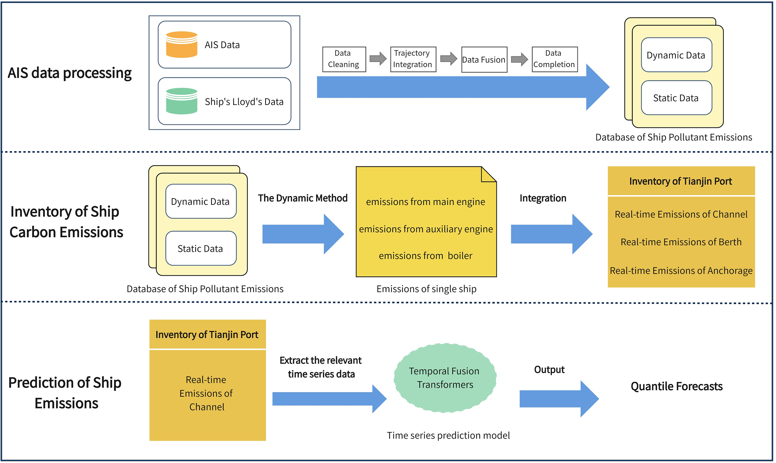
Figure 1 Research flow diagram.

2 Materials and methods

2.1 Overview of the research area and data sources

The research area was the sea around Tianjin Port in China (38.64°N–39.24°N, 117.35°E–118.35°E. The layout of Tianjin Port is shown in Figure 2. Tianjin has unique geographical properties, and it is an important sea link connecting north and south, east and west, and China and abroad. Tianjin Port, located in the Binhai New Area of Tianjin, is the largest comprehensive hub port in northern China. In 2021, container throughput exceeded 20 million twenty-foot equivalent units (TEUs), ranking it eighth in the world (Wang, 2022). It is also the main port for foreign trade exports and an important entry point for foreign materials and equipment (Niu, 2022)

FIGURE 2

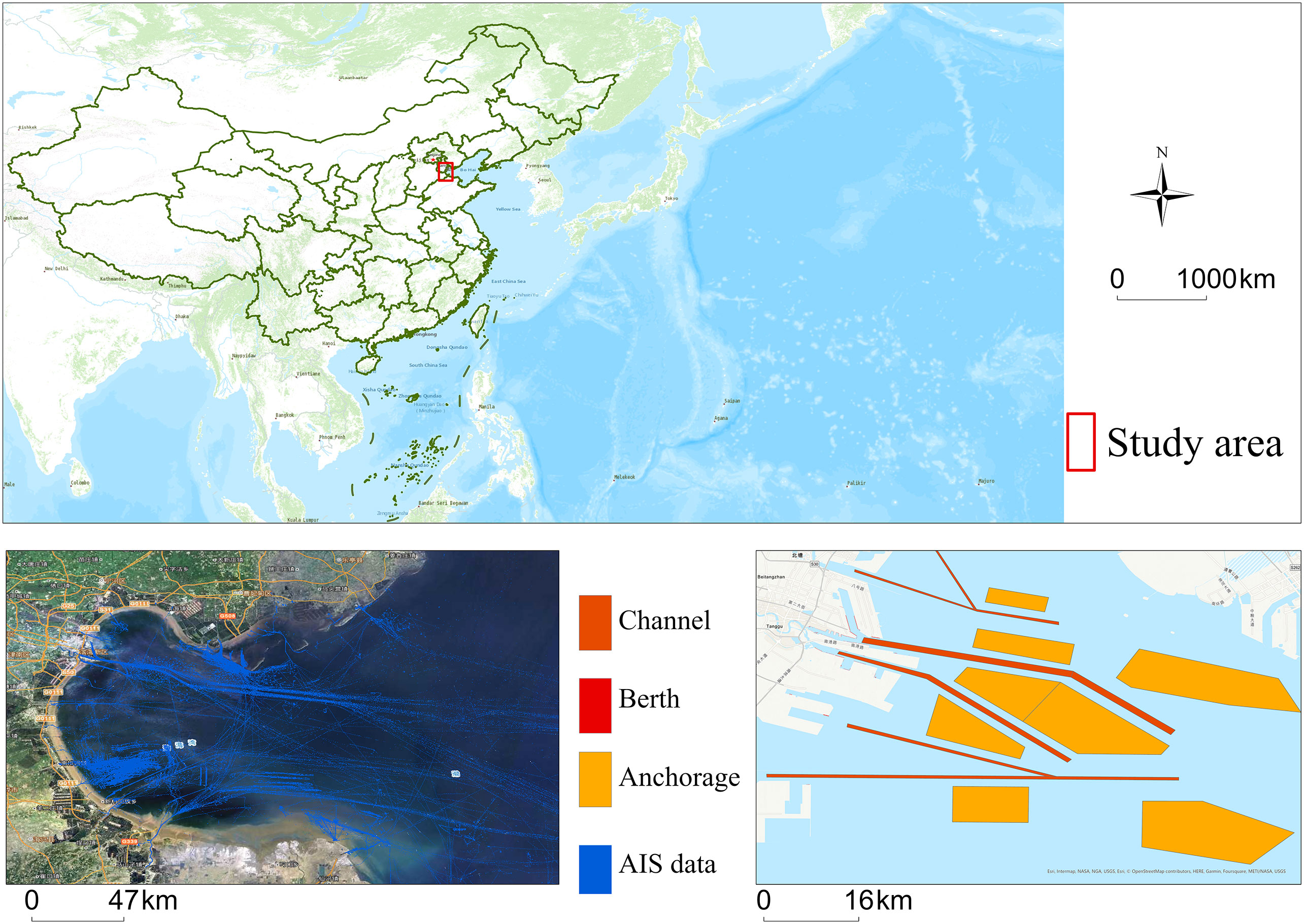
Figure 2 Layout of research area -- Tianjin Port.

We used the AIS data to estimate ship carbon emissions at Tianjin Port with high spatiotemporal resolution. The CO₂ emissions were analyzed in multiple dimensions to provide decision-making support for relevant management bodies. AIS sends signals at frequencies of every 3 seconds to a few minutes that include detailed information on ship speed and location. High-precision AIS data ensure the accuracy of ship emission predictions (Weng et al., 2019). AIS signals can be interpreted into static information, dynamic information, voyage information, and security information for analysis (Chen et al., 2021a). Static information includes ship’s MMSI, ship name, ship type, ship length, ship width, ship tonnage, and the place of ship registration. Dynamic information includes ship position (latitudinal and longitudinal coordinates), course, speed, and time (UTC seconds, indicating the time of report generation) (Weng et al., 2019). Voyage information includes the draft of the ship, the type of dangerous goods carried by the ship, the port of destination and the passage plan. Safety information mainly refers to navigation rights information related to ship navigation (Chen et al., 2021a).

The research data consisted of 2018 AIS data for ships, including 7 channels, 8 anchorages, and 205 berths in Tianjin Port that were combined with Lloyd’s data and pollutant emission parameters. The channels were respectively Dagang Port channel, Beitang Port channel, Xingang channel outer section, Xingang channel inner section, Dagusha channel, Gaoxaling Port channel and Beitang Port branch channel. There were 26 ship types, including dry bulk carriers, container ships, oil product ships, rescue ships, roll on–roll off (ro-ro) ships, passenger ships, ore carriers, tugboats, liquid chemical carriers, and fishing boats. The pollutant of interest was greenhouse gas emissions of CO₂.

2.2 AIS data processing of ships

We used the dynamic method to calculate CO2 emissions from ships. The quality of AIS data affects the accuracy of the research results. Information loss, error, data duplication, and abnormality can occur in AIS data transmission and collection due to sensor characteristics, signal interference, transmission channel congestion and other reasons (Wu et al., 2017). These forms of data interference can corrupt subsequent data mining and analysis and affect the analysis results. We therefore first undertook data cleaning, trajectory integration, data transformation, data fusion, data extrapolation and other operations on the AIS data and preprocessed ship data to avoid adversely affecting the results by poor data quality. Data processing procedures are shown in Figure 3:

FIGURE 3

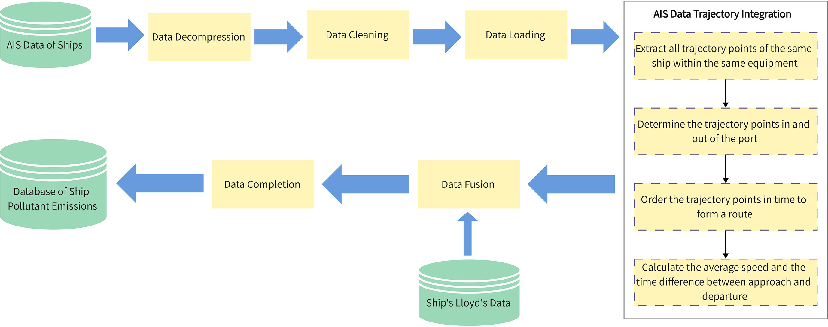
Figure 3 Diagram of data processing.

2.2.1 Data cleaning

Given the problems previously identified, such as faults, errors, and discontinuity, that may exist in the storage and management of massive AIS data, as well as the problems such as data loss, abnormality, truncation, and rate instability that may exist in multi-channel incremental AIS data access, direct use of original data in research and analysis will certainly affect the accuracy of the results. To ensure satisfactory analysis results and meet the requirements of ship carbon emissions traceability, data cleaning is necessary to remove data not conforming to common sense based on reasonable ranges in various fields (Wang and Li, 2021).

Anomalies in ship speed were determined by comparing ship’s real-time speed and ship’s maximum speed. If the real-time speed was greater than the maximum speed, the ship trajectory point was deleted as a speed anomaly. The course of a ship is 0°–360°. If the course was outside this range, the data point was deleted. If the tracked position of the ship was outside the coordinates of Tianjin Port, the data point was deleted. If the MMSI did not have 9 digits, it was deleted. If the latitude or longitude was empty, the latitude was >90° or<−90°, or if the longitude was >180° or<−180°, the data point was deleted. In addition, data points for locations outside the research scope, data points for times outside the research scope, and duplicate data points were also deleted (Feng et al., 2022). The cleaned data were imported into the database for subsequent processing and analysis.

2.2.2 AIS data track integration

AIS sends signals with a frequency of 3 seconds to a few minutes, so the dynamic data recorded by AIS forms a massive point dataset with coordinates, and the quantity of data for Tianjin Port in 2018 was therefore extremely large. This was rather inconvenient for subsequent processing, and did not immediately represent ship trajectories. It was therefore necessary, for all ships, to extract the critical trajectory points describing the original trajectory of the ship from the dense data points and to create the shipping route by ordering the data points in a time sequence (Wang and Li, 2021) to facilitate the calculation of massive AIS data.

In this paper, route extraction was performed first. All track points for the same MMSI in the same port facility (channel, anchorage, berth) at Tianjin Port were extracted, and the port entry and exit points of the ship were determined. The track points from the entry position to the departure position were sorted according to the data sampling time to create the route of the ship, and the time difference between entry and departure was calculated. The average of the speeds at each track point was taken to be the average speed for the route. AIS data after incorporating the trajectory included ship MMSI, ship type, place of registration, ship captain, ship width, entry time, departure time, ID and name of the port facility used, sailing time, average sailing speed and other information. Ship activity in a port facility was represented by a piece of data. After track integration of the Tianjin Port data in 2018, a total of 20 361 anchorage data points, 70 572 channel data points, and 47 145 berth data points were used in the calculation of the ship carbon emissions inventory.

2.2.3 Data fusion and completion

The Lloyd’s data contained basic information about the ship, such as the MMSI, the year of construction, the ship type, the place of registration, the maximum rated continuous power of main engines, the speed of the main engine (>1000 rpm for high-speed engines, 300–1000 rpm for medium speed engines, and<300 rpm for low speed engines), the main engine manufacturer, the maximum rated power of auxiliary engines, number of engines, designed maximum speed, and fuel type.

Using the MMSI code as a key, we obtained static vessel information from the Lloyd’s registry such as the maximum rated continuous power of the main engine, the maximum rated power of the auxiliary engine(s), ship manufacturer, the tonnage class, the speed of the main engine, the designed maximum speed, and the age of the vessel and then matched and incorporated these data with the AIS data after integrating the vessel trajectory.

In cleaning these data, based on a statistical analysis of ships in Tianjin Port, we eliminated records when the AIS data showed a Tianjin Port channel navigation time >2 h, anchorage time >20 d, or at berth time >4 d.

Statistical averages or curve fitting were used to extrapolate data that were not included in the Lloyd’s database to establish a complete database of ship carbon emissions. Ship construction date and ship manufacturer were completed using the statistical method of corresponding data mode in Lloyd’s database. Ship tonnage and ship main engine speed were obtained by calculating the mean value of corresponding data in the Lloyd’s database. The maximum rated power of the main engine and maximum rated power of the auxiliary engine were obtained by various methods, depending on the context of the missing information.

Main engine power was extracted from the Lloyd’s database for most ships. Engine power data for ships that were not found in the database were extrapolated in order to provide accurate pollution estimates. It was assumed that the power of the main engine was related to the type of ship and its gross tonnage. Engine power of ships for which no such data had been recorded was then completed by Lloyd’s data referring to the actual situation (Trozzi, 2010; Ng et al., 2013; Chen et al., 2017). For example, the average main engine power of ships with similar gross tonnage was used as the main engine power of ships, for which there was no main engine power data but available gross tonnage data. The average main engine power of ships with similar width and height was used as the main engine power of ships, for which there were neither main engine power data nor gross tonnage data. For ships with only MMSI number and ship type data available, the average main engine power of all ships of the same type in Tianjin Port was used as the main engine power. For ships with only MMSI number available, the average main engine power of all ships in Tianjin Port was used as the main engine power (Weng et al., 2019).

Missing auxiliary engine (AE) power can be predicted using the ratio of AE power to main engine (ME) power of a particular ship type (Trozzi, 2010; Chen et al., 2017). AE power data were created using ME–AE power ratios of different types of ships obtained from the China Knowledge Centre for Engineering Sciences and Technology, 2016 (China Knowledge Centre for Engineering Sciences and Technology, 2016). See the Supplementary Materials for detailed information.

2.3 Creation of a high-resolution CO₂ emissions inventory from ship data

For the estimation of greenhouse gas CO₂ emissions from ships, the top-down dynamic method was adopted in this study. The total energy output of each ship (kW·h) was multiplied by an emission factor that was specified in g/kW•h. The estimated value was then modified using the corresponding emission factor correction coefficient to produce the carbon emissions from the main engine, auxiliary engine, and boiler of a single ship respectively. We calculated CO₂ emissions for individual ships in each channel, anchorage, and berth using geographical information for Tianjin Port and then combined the CO₂ emissions of all ships at different times for the entire port area to produce real-time emissions for the different port facilities. Then, a high-resolution CO₂ emissions inventory of ships was created.

CO₂ emissions were calculated for each of 26 different ship types, including dry bulk carriers, container ships, refined oil carriers, rescue ships, ro-ro ships, and fishing boats. Emissions were classified by engine type (main engine, auxiliary engine, and boiler) and vessel operating mode (cruising, slow sailing, maneuvering, at anchor, and berthed) (Liu et al., 2016).

Air pollutants are emitted from ships in port mainly from marine engines, primarily the main engine, auxiliary engine(s) and boiler, which have different functions. The main engine provides propulsion power for the ship, the auxiliary engine powers lighting, air conditioning, refrigeration and other electrical equipment for the ship, and the boiler provides hot water or steam for driving equipment on the ship. Engines are generally divided into five categories by speed and type: low speed diesel engine (SSD), medium speed diesel engine (MSD), high speed diesel engine (HSD), gas turbine (GT) and steam turbine (ST). Large vessels usually have an SSD with a maximum speed<350 rpm as the main engine. An MSD with a maximum speed 350–1000 rpm is usually the main or auxiliary engine of large ships. HSDs with a speed >1000 rpm are used as main engines in small ships or auxiliary engines in large ships (China Knowledge Centre for Engineering Sciences and Technology, 2016). The carbon emission calculations for main and auxiliary engines and boilers in a single ship are as follows (Liu et al., 2016).

2.3.1 Emissions of ship main engine

The following equation calculates pollutant emissions of the main engine:

$\begin{array}{ll}Ei=MCR\times LF\times Act\times EFi\times FCF\times CF\times {10}^{-6}& (1)\end{array}$

where Ei is the estimated CO₂ emission of the main engine (t); MCR is the maximum continuous rated power of the main engine (kW); LF is the load coefficient of the main engine (dimensionless) and is calculated by:

$\begin{array}{ll}LF={(\frac{Speed\_Actual}{Speed\_Max})}^3& (2)\end{array}$

where Act is the sailing time of the ship (h); EFi is the emission factor of CO₂ (g/kW·h), detailed in the Supplementary Material; FCF is the fuel correction coefficient (dimensionless) for fuel types RO (2.7% S), HFO (1.5% S), MGO (0.5% S), MDO (1.5% S), MGO (0.1% S); FCF for CO₂ is 1; and CF is the low load adjustment factor for the main engine (dimensionless), detailed in the Supplementary Material.

2.3.2 Emissions of auxiliary engine

The equation to calculate pollutant emissions of an auxiliary engine is:

$\begin{array}{ll}Eai=A\_MCR\times LF\_a\times Act\times EFai\times FCF\_a\times {10}^{-6}& (3)\end{array}$

where Eai is the estimated CO₂ emission of auxiliary engine powered machinery (t); A_MCR is the maximum continuous rated power of the auxiliary engine (KW), which is obtained from the Lloyd’s database or, if not available, calculated by the ratio of the power of the auxiliary engine to the maximum continuous rated power of the main engine, by:

$\begin{array}{ll}A\_MCR=AMR\times MCR& (4)\end{array}$

where AMR is the ratio of the power of auxiliary engine to the maximum continuous rated power of the main engine, detailed in the Supplementary Materials; MCR is the maximum continuous rated power of the main engine (KW); LF_a (dimensionless) is the load factor of the auxiliary engine, determined according to the type of ship and its sailing state (see Supplementary Materials); Act is the operating time of the auxiliary machinery of the ship (h); EFai is the emission factor of CO₂ (g/kW·h) (see Supplementary Materials for details); and FCF_a (dimensionless) is a fuel correction coefficient for RO (2.7% S), HFO (1.5% S), MGO (0.5% S), MDO (1.5% S), MGO (0.1% S); FCF_a for CO₂ is 1.

2.3.3 Boiler emissions

The equation to calculate pollutant emissions from a ship boiler is:

$\begin{array}{ll}Ebi=B_{Energy}\times Act\times EFbi\times {10}^{-6}& (5)\end{array}$

where Ebi is the CO₂ emission from the boiler (t); B_Energy is the load power of the boiler (KW); the boiler is usually started only when the main engine load is ≤20% and the boiler is inactive when the ship is sailing normally at sea; the boiler load power data are detailed in the Supplementary Materials; Act is the startup and operating time of the boiler (h); and EFbi is the CO₂ emission factor of the boiler, 970 g/kW·h.

After estimating the carbon emissions generated by the main engine, auxiliary engine, and boiler of a single ship along a single course track, the carbon emissions of the activity of a ship in each Tianjin Port facility can be obtained by summing them, and the real-time emissions of each type of equipment in Tianjin Port in different time periods can be obtained.

2.4 Ship emissions prediction model based on the attention mechanism

A recently developed attention-based deep neural network (DNN) architecture, the time fusion transformer (TFT) (Lim et al., 2021), was used in this study to predict carbon emission characteristics of ships in Tianjin Port for several periods. This model has significantly improved the performance of various applications over existing models, such as ARIMA, ETS, TRMF, DeepAR, DSSM, ConvTrans, Seq2Seq, and MQRNN. The major constituents of TFT are gating mechanisms, variable selection networks, static covariate encoders, temporal processing, and prediction intervals.

Based on the established high-resolution carbon emissions inventory, static and time-varying variables related to the prediction target were extracted for learning and training. While multiple variables may be available, their relevance and weight are usually unknown. TFT selects the relevant input variable at each time step through variable selection networks. All static, historical, and future inputs use independent variable selection networks. Apart from providing insight into the most important variables of the prediction problem, variable selection removes any unnecessary noise inputs that can degrade performance.

The TFT model integrates information from static metadata, modulates temporal dynamic variables by encoding context vectors, and thus integrates static features into the network. Independent GRN encoders were adopted to generate context vectors that were wired to different locations of the temporal fusion decoder. Static covariates often significantly affect temporal dynamics, so a static richness layer was introduced to enhance temporal characteristics with static metadata. All statically rich time characteristics applied multi-head attention in each prediction (N = τ_max + k +1) to extract long-term dependent information. Decoder masking (Vaswani et al., 2017; Li et al., 2019) was employed to ensure that each temporal dimension only focuses on its previous features. We used GRN to the output of the self-attention layer, which is similar to the static enrichment layer.

To capture both long-term and short-term time relationships from time-varying inputs and weight information at different moments, TFT uses the sequence-to-sequence layer for local processing, and uses multi-head attention to capture long-term dependence.

TFT uses linear transformations of the output of the temporal fusion decoder to generate forecast intervals by simultaneously predicting different percentiles at each time step.

$\begin{array}{ll}\widehat{y}(q,t,\tau )=W_q\tilde{\psi }(t,\tau )+b_q& (6)\end{array}$

where W_q ∈ ℝ^1×d and b_q ∈ ℝ are the linear coefficients of quantile q. The predictions are generated only for future periods {1, ... ,τ_max}.

The model’s overall architecture is shown in Figure 4 (Lim et al., 2021).

FIGURE 4

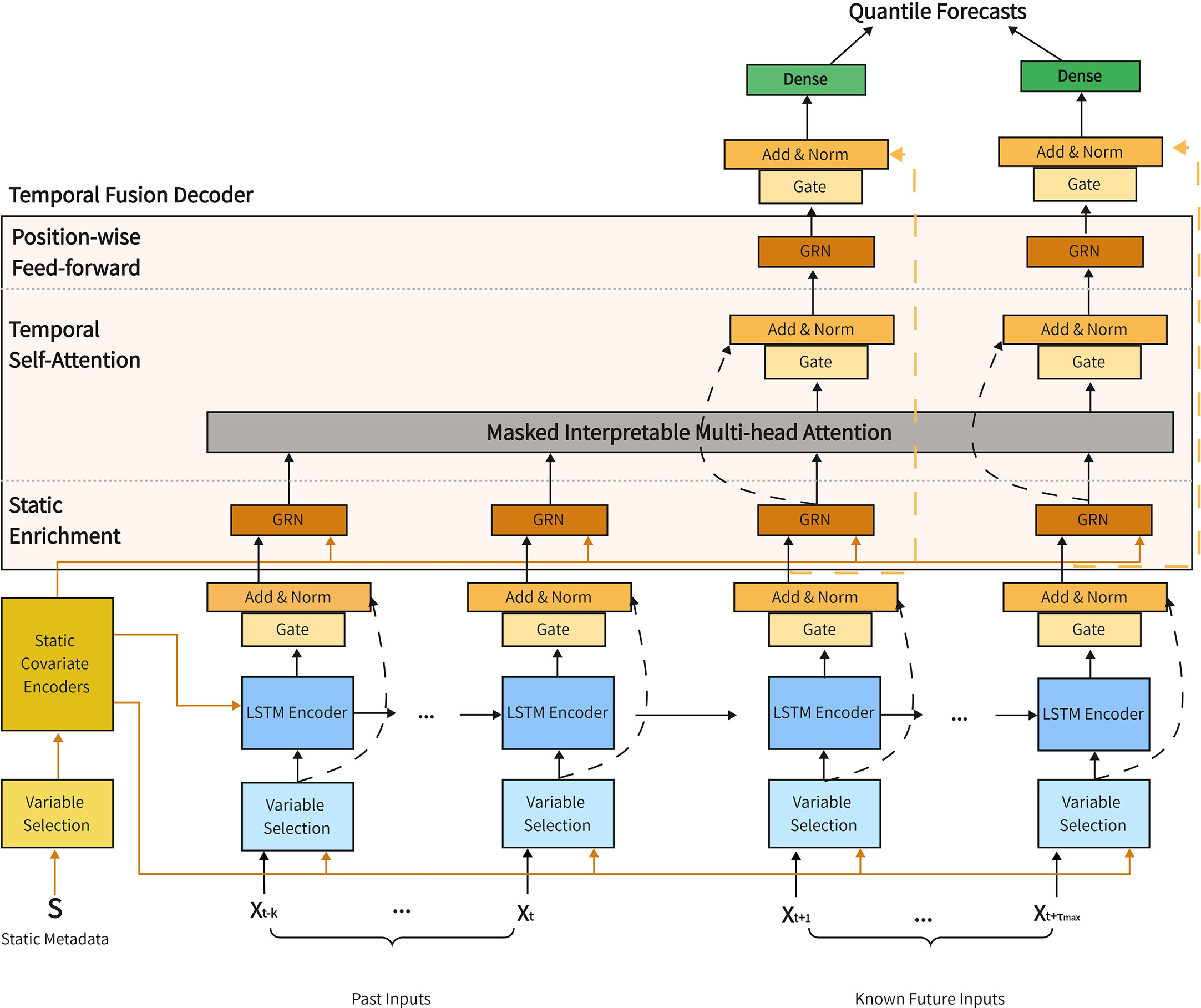
Figure 4 TFT architecture.

The remainder of this section is drawn from Lim et al. (2021) under the terms of the Creative Commons CC-BY 4.0 license.

2.4.1 Gated residual network

The exact relationships between model inputs and the target predicted values are often unknown in advance, making it challenging to determine the degree of nonlinear processing required. To give the model the flexibility to apply nonlinear processing only where needed, gated residual network (GRN) was used. The GRN takes the primary input a and an optional context vector c to produce:

$\begin{array}{ll}GR{N}_{\omega }(a,c)=LayerNorm(a+GL{U}_{\omega }({\eta }_1))& (7)\end{array}$

$\begin{array}{ll}{\eta }_1=W_{1,\omega }{\eta }_2+b_{1,\omega }& (8)\end{array}$

$\begin{array}{ll}{\eta }_2=ELU(W_{2,\omega }a+W_{3,\omega }c+b_{2,\omega })& (9)\end{array}$

where ELU is the exponential linear unit activation function (Clevert et al., 2016), η₁ ∈ ℝ^dmodel, η₂ ∈ ℝ^dmodel are the intermediate layers, LayerNorm is the standard normalization (Lei Ba et al., 2016), and ω is the weight sharing index. When W_2,ωa + W_3,ωc + b_2,ω >> 0, ELU activation will act as an identity function. When W_2,ωa + W_3,ωc + b_2,ω<< 0, ELU activation will produce a constant output, producing linear layer behavior.

2.4.2 Multi-head attention

TFT uses a self-attention mechanism to learn the long-term relationship across different time steps. The mechanism is modified in the transformer-based architecture. The range value of attention mechanism V ∈ ℝ^N×dV based on the relationship between keys K ∈ ℝ^N×dattn and queries Q ∈ ℝ^N×dattn is:

$\begin{array}{ll}Attention(Q,K,V)=A(Q,K)V& (10)\end{array}$

where A is a normalization function. A common choice is scaled dot product attention (Vaswani et al., 2017):

$\begin{array}{ll}A(Q,K)=Softmax(Q{K}^T/\sqrt{d_{attn}})& (11)\end{array}$

To improve the learning ability of the standard attention mechanism, multi-head attention was proposed, and different heads were used for different representation subspaces:

$\begin{array}{ll}MultiHead(Q,K,V)=[H_1,\dots ,H_{mH}]W_H& (12)\end{array}$

$\begin{array}{ll}{H}_h=Attention(Q{W}_Q^{(h)},K{W}_K^{(h)},V{W}_V^{(h)})& (13)\end{array}$

where W_K^(h) ∈ ℝ^{dmodel×dattn}, W_Q^(h) ∈ ℝ^{dmodel×dattn}, W_V^(h) ∈ ℝ^dmodel×dV are the header weights of keys, queries, values, and W_H ∈ ℝ^{(Mh·dV)×dmodel} is the output from the linear combination of all headers H_h.

Assuming different values are used for each header, individual attention weights do not indicate the importance of a particular feature. We therefore modified the multi-head attention to share the values in each head and sum all heads:

$\begin{array}{ll}InterpretableMultiHead(Q,K,V)=\tilde{H}{W}_H& (14)\end{array}$

$\begin{array}{ll}\begin{array}{l}\tilde{H}=\tilde{A}(Q,K)V{W}_V=\left\{\frac{1}{H{\sum }_{h=1}^{mH}A(Q{W}_Q^{(h)},K{W}_K^{(h)})}\right\}V{W}_V\\ =\left\{1/H\sum _{h=1}^{mH}Attention(Q{W}_Q^{(h)},K{W}_K^{(h)},V{W}_V)\right\}\end{array}& (15)\end{array}$

where W_V ∈ ℝ^dmodel×dV is the weight of a value shared across all headers, and W_H ∈ ℝ^dattn×dattn is used for the final linear mapping. Each head can learn different time patterns and focus on the characteristics of a set of common input features simultaneously. It can be interpreted as Eq. (14) with attention weighting to form the simple combination matrix Ã(Q, K).

3 Results

3.1 Spatial and temporal distribution

3.1.1 Time distribution rule

The carbon emissions of the main engine, auxiliary engine and boiler under different working conditions were estimated for ships in channels, berthed, and at anchorage in the area defined in the study as Tianjin Port in 2018. Ship CO₂ emissions for each month are shown in Figure 5. Detailed emission data are shown in the Supplementary Materials.

FIGURE 5

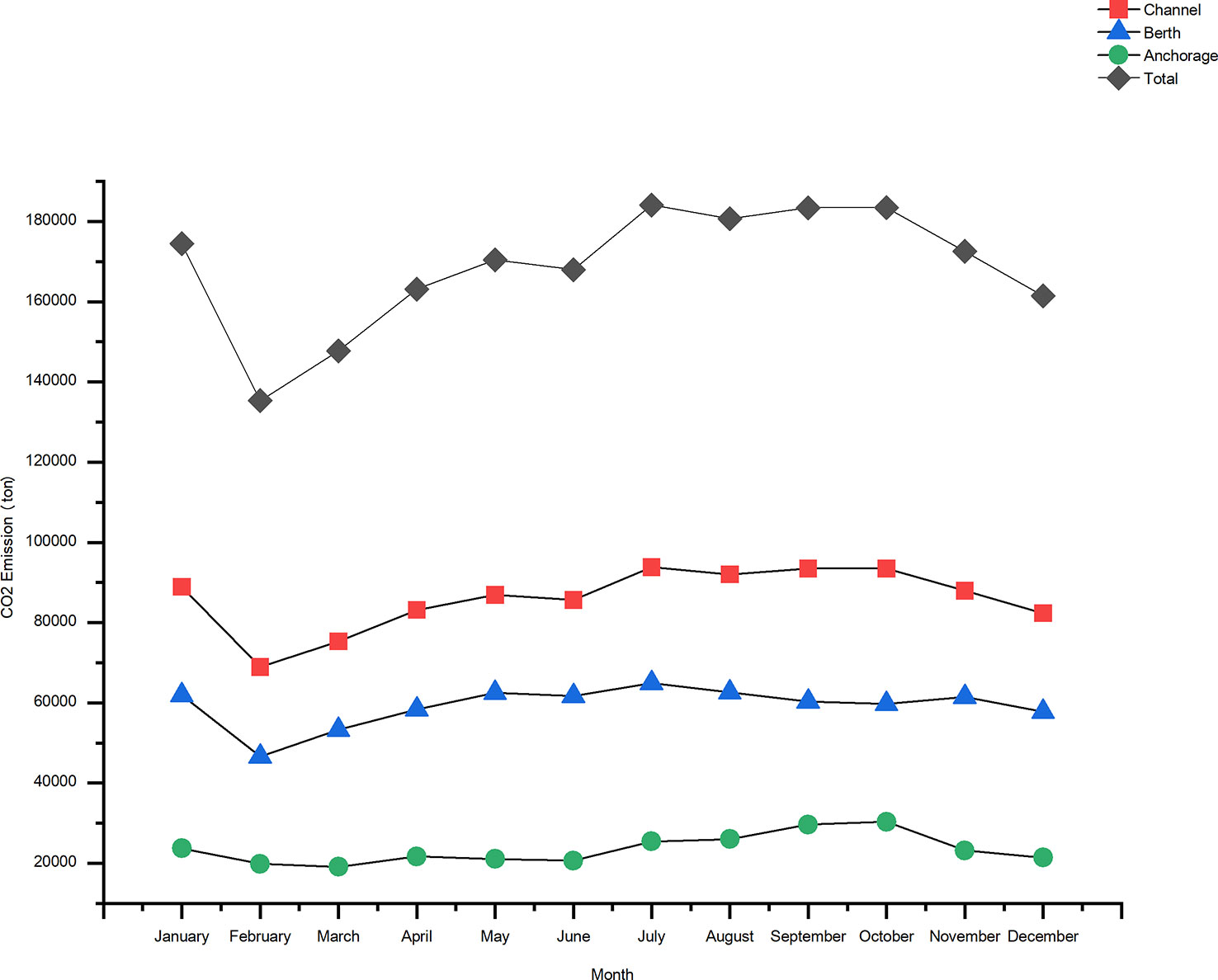
Figure 5 CO₂ emissions from ships in Tianjin Port in 2018.

Figure 5 shows that CO₂ emissions were high in July, August, September, and October, and peaked in July. In January, preceding the Chinese New Year, the dry bulk trade volume is high, resulting in increased carbon emissions even during the winter season. February is traditionally the off-season of the Chinese New Year; supply and demand are weak, trade volume decreases, and ship emissions decrease accordingly (Zhang and Yan, 2019). Emissions were low in June when the Bohai Bay area was closed to fishing and shipping was strictly controlled. In addition, the trade war between China and the United States in 2018 reduced the volume of trade routed through Tianjin Port. In March, 2018, the former U.S. President Trump signed a memorandum imposing heavy tariffs on imported steel and aluminum, initiating the trade dispute between China and the United States, which affected commodity prices and reduced market confidence. In response, the Chinese government continually released reform signals, which greatly alleviated market concerns (Zhang and Yan, 2019), and trade volume rebounded. However, changes in the international political and economic environment are complex, and the effects on trade were inevitably longer term. For example, in September–December 2018, Tianjin Port imported no soybeans from the United States (Tianjin Customs District P. R. China, 2019).

In most years, ice starts to form in the port in early December and lasts until February of the following year. The most severe period of ice is generally from early January to the end of February (Xia, 2006). Tianjin Port experienced severe ice formation in late January and early and mid-February of 2018. The coastal ice of Tianjin Port melted in late February, 2018 (Tianjin Municipal Bureau of Planning and Natural Resources, 2018). Thus, in January and February, November, and December, port traffic was reduced due to sea ice conditions, and ship pollutant emissions decreased. The government, along with other relevant departments, needs to promptly adjust their allocation of human resources and regulation efforts to manage high emissions between July and October, and prepares for the fishing ban and the winter sea ice period.

3.1.2 Spatial distribution

The geographical coordinates in ship AIS data enabled us to combine real-time emissions and shipping trajectories to analyze the characteristics of carbon emissions. We therefore summed the emissions of all shipping trajectories for each grid box and mapped the spatial distribution of ship carbon emissions in Tianjin Port in 2018 using GIS (Figure 6). The figure clearly identifies areas with high emissions, with much of the greatest traffic density occurring within a small part of the total area, such as the Main Shipping Channel of Tianjin Xingang Fairway and Dagusha Channel.

FIGURE 6

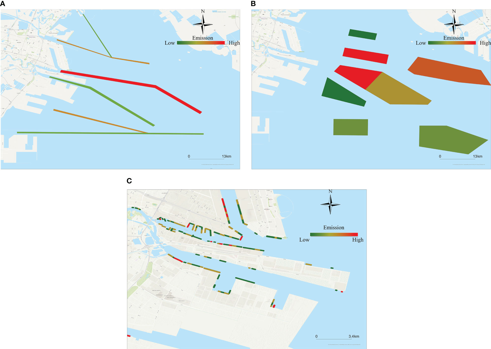
Figure 6 Spatial distribution of carbon emissions from ships in Tianjin Port in 2018. (A) channel; (B) anchorage; (C) berth.

The Master Plan of Tianjin Port (2021–2023) shows that the port will focus on building a layout of “one port and nine districts” in the future. The nine districts are Northern Xinjiang port area, East Xinjiang port area, South Xinjiang port area, Dagu port area, Gaoxaling port area, Dagang port area, Haihe port area, Beitang port area, and Hangu port area. The plan goal is to speed up the construction of the northern international shipping center. Northern Xinjiang will focus on the development of modern logistics, bonded warehousing, finance and trade, and shipping services. Dongjiang will mainly process container transportation. Southern Xinjiang is for coal, iron ore, oil and oil products and other bulk cargo in transit. Dagu will mainly be used for shipbuilding and ship repair, equipment manufacturing, grain and oil processing, and other transportation industries. Gaoshaling will serve the equipment manufacturing industry in the near future, and in the more distant future will take in the harbor industry and materials transportation into the hinterland. Dagang serves the petrochemical industry of Nangang Industrial Zone in the near future and bulk cargo transportation in the longer term. Haihe serves the development of waterfront industry, transportation of construction materials, and tourist ships and transport. Beitang will mainly serve passenger transport and coastal tourism. Hangu will serve the aquatic products industry in this region, focusing mainly on the transportation of groceries and cold chain materials (Cui, 2010).

Pollutant emissions near all land port areas and the channels of Tianjin Port are generally very high. Xingang channel outer section is a high emission area, contributing about 64.9% of all channels’ emission. The carbon emissions in the Beitang Port channel and Xingang channel inner section are each clearly higher than in other channels. This necessitates port regulatory authorities to plan reasonably, taking into consideration the emission characteristics of the port cargo structure and port characteristics. This ensures optimal utilization of all areas without overloading, thereby avoiding unnecessary emissions arising from traffic congestion or protracted waiting times for goods loading and unloading in certain areas.

3.2 Characteristic ship attributes

3.2.1 Ship type

The count and throughput of each type of ship are different, so the quantities of CO₂ emitted are also different. Figure 7 shows the pollutant emissions from different types of ships in 2018.

FIGURE 7

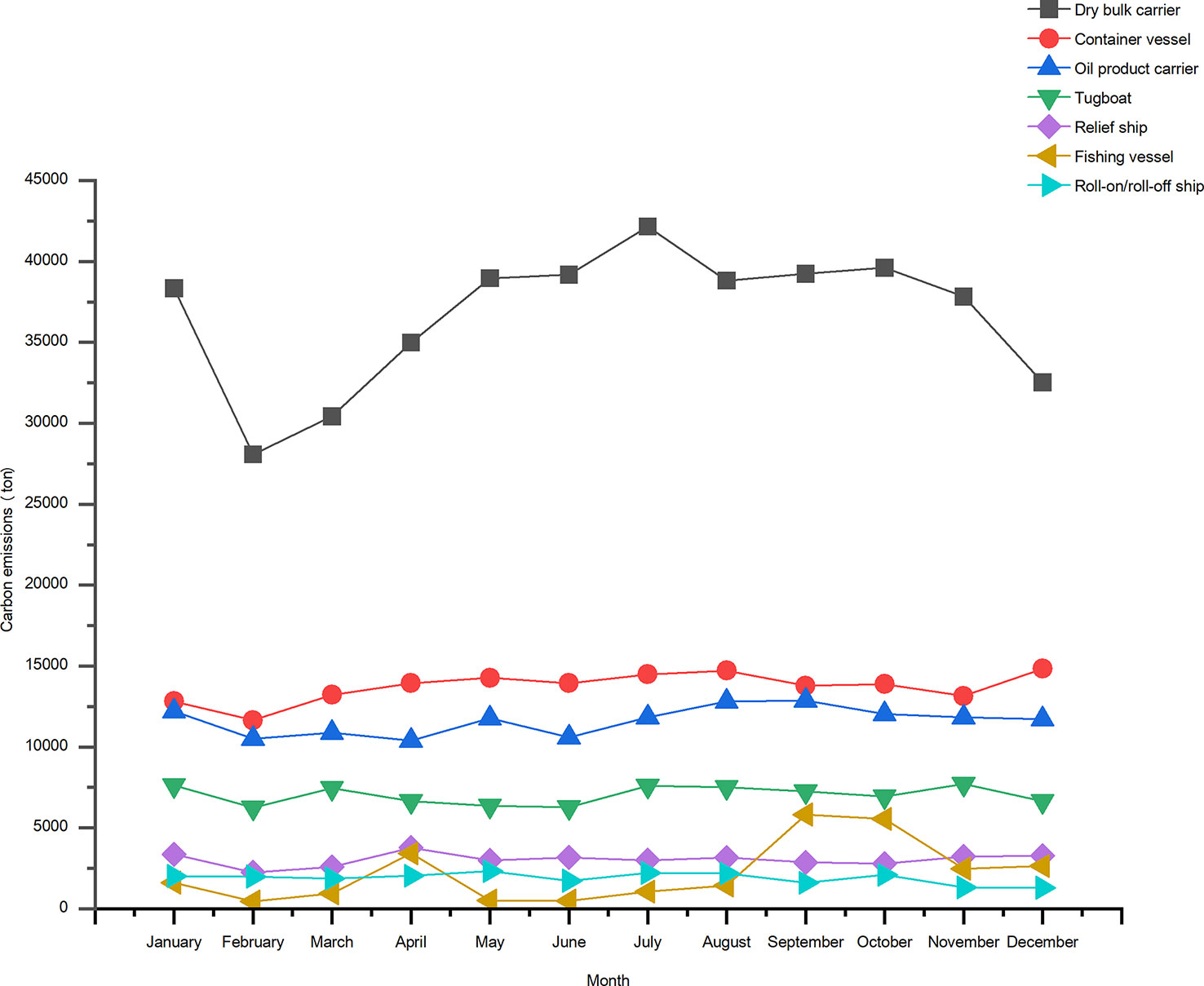
Figure 7 Changes in emissions from different types of ships in 2018.

Figure 7 shows that dry bulk carriers produced the greatest quantities of carbon emissions, followed by container ships and oil product carriers. Each of these ship types accounted for more carbon emissions than the other ship types combined; other types of ships, such as fishing boats and ro-ro ships produced relatively low carbon emissions. The Chinese Spring Festival and the trade dispute between China and the United States together reduced the supply and demand of dry bulk cargo, which decreased in February and March. These events not only affected trading volume, but also decreased ship carbon emissions. Since Bohai Bay is closed to fishing most of the year, the carbon emissions of fishing boats were concentrated into September and October, whereas the monthly emissions of other types of ships were relatively constant.

Figure 8 shows the monthly percentage contribution of pollutant emissions for each type of ship in Tianjin Port in 2018.

FIGURE 8

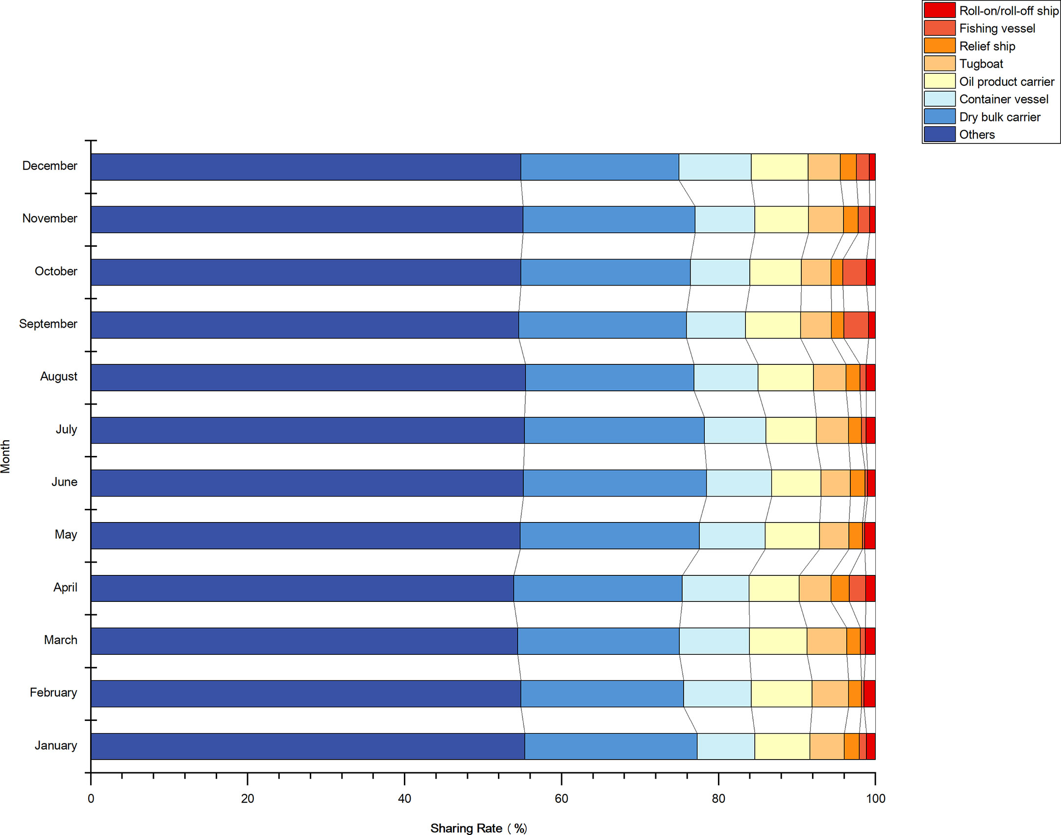
Figure 8 Pollutant emission share of different types of ships in each month of 2018.

Figure 8 shows that the pollutant emissions of dry bulk carriers, container ships, and oil product carriers were relatively large. The three types of ship, as the main types of vessels primarily used in international shipping, together contributed 36.76% of total carbon emissions. Of these three types of ship, dry bulk carriers made the greatest contribution, with a maximum of 21.74%, and the contribution of container ships, which was second to dry bulk carriers, was 8.13%. Oil product ships contributed 6.89% and tugboats 4.16%.

Tianjin Port is the largest port in northern China, and it is the gateway to Beijing’s shipping trade. It is a comprehensive international port with complete cargo facilities. It has formed a cargo specialty structure with containers, crude oil and oil products, ore, and coal as its “four pillars” and steel and grain as “a group of key points”, making it one of the largest and most comprehensive ports in the Bohai Rim region. Tianjin is also China’s largest coke export port in terms of tonnage, the second largest iron ore import port, and the largest container trunk port in northern China. Thus, many container ships visit the port. Container ships travel at high speed, carry heavy loads, and have more powerful engines than other types of ship; the carbon emissions of a single container ship is much greater than that of any other type of ship. There was no significant difference in carbon emissions between dry bulk carriers and other types of ship. However, there were more dry bulk carriers than any other type of ship and they accounted for about 31% of the total number of ships, with a maximum of 2765 ships in July and a minimum of 1797 ships in February. Therefore, the total carbon emissions of dry bulk carriers were greater than those of container ships. The number of tugboats was the second highest, reaching a maximum of 1579 in August. Ship arrivals in each month are provided in the Supplementary Materials.

In accordance with the Energy Efficiency Operational Indicator (EEOI) as defined by the International Maritime Organization and past research, ships with a deadweight tonnage of less than 50,000 typically manifest greater carbon intensity compared to other ships (Walsh and Bows, 2012).Enhancing the transportation capacity of containers will diminish the amount of fuel needed for their transit, ultimately curtailing greenhouse gas emissions from shipping (Li et al., 2023). To reduce ship exhaust emissions, a significant number of shipping companies are contemplating the utilization of larger or medium-sized ships (Ammar and Seddiek, 2020).This necessitates relevant regulatory authorities, shipping companies, and shippers to enter into agreements to specify the types of ships to transport each type of cargo, to employ large ships for cargo transport as much as possible, and to strictly monitor the CO₂ emissions from different types of ships. Local governments should reach agreements with local ports and terminals, plan port structures and cargo loading and unloading mechanisms sensibly, and minimize unnecessary CO₂ emissions. Concerning ship age, since newer ships are typically equipped with superior carbon efficiency and emit lower emissions, relevant departments could enhance standards for in-service ships by mandating the scrapping of ships that have exceeded their service life.

3.2.2 Place of ship registration

Ships are a major source of pollution in inland waterway navigation, but they also may be important protectors of the inland waterway environment, because they can reduce pollutant emissions through the adoption of clean energy technologies. However, the extra cost of clean energy technology can inhibit the participation of shipping enterprises in environmental management of inland rivers. Thus, government will be required to strengthen environmental oversight. The decision of shipping enterprises to use clean energy is therefore closely related to government management and control (Xiao et al., 2022).

The place of ship ownership is an important aspect of understanding the source of carbon emission, which is related to taxation through carbon emission trading. An analysis of CO₂ emissions can be a proxy for the analysis of other pollutants. In combining AIS data with ship data, we obtained the nationality and registration of ships in Tianjin Port in 2018. Ships registered in China, Hong Kong, and Liberia were responsible for the greatest carbon emissions in the port, followed by ships registered in the Marshall Islands and Singapore. Figure 9 shows the percentage emissions by ships registration; detailed emission data and emission ranking of ships from different countries and regions are shown in the Supplementary Materials. CO₂ emissions from ships registered in countries other than China were about 33.5% of the total, which indicates that there is a need to reduce and control emissions from both Chinese-registered ships and also foreign-registered ships.

FIGURE 9

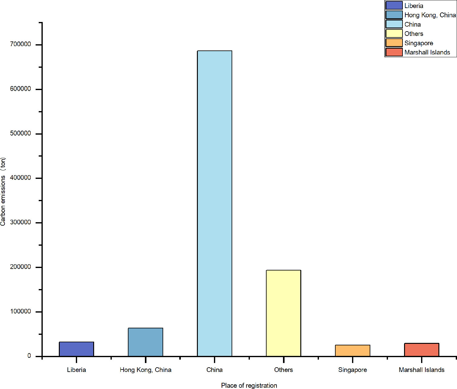
Figure 9 Carbon emissions from ships by place of registration.

Rehmatulla (2014) revealed that, on average, more than 50% of the charter market in the dry bulk sector operates on a time charter basis, where fuel costs are borne by the charterer. In contrast, shipping companies that employ clean energy may receive construction subsidies and carbon emissions trading subsidies during the early stages of a ship’s service life. This assistance can help offset the costs associated with energy procurement and material transformation.Local governments are encouraged to capitalize on investments in funds, technology, and human resources. They ought to adopt strategies that attract more investors to endorse clean energy-related projects and collaborate with local ports and terminals to prioritize actions such as loading and unloading clean-energy ships (Xu et al., 2021). Incorporating the use of cleaner ships into credit limit considerations could accelerate the market-driven strategy for cleaner ships (Liu et al., 2019). In addition, authorities need to conscientiously address ships that illicitly discharge pollutants.

3.3 Navigational status characteristics

Ship activity can be divided into five modes according to the speed of the vessel: cruising, slow speed, maneuvering, anchoring (at anchorage), and berthed.

The main engine of the ship provides power for ship navigation; the propeller drives the ship by absorbing and dissipating the power provided by the main engine. The main engine must be operating while the ship is cruising, running at slow speed and maneuvering, and in these modes of operation, carbon emissions are at a maximum. Auxiliary engines provide electric energy for ships during navigation. Since the research area we selected surrounds the port, the average sailing speed of ships in the research area was less than if we had selected ships at sea. Thus, in the research area, compared to vessels at sea, the emissions of main engines are proportionately reduced, and the emissions of auxiliary engines are proportionately increased. Carbon emissions of auxiliary engines in the research area accounted for about one-third of the total, and were also the main source of ship carbon emissions. The boiler operates mainly when the main engine is under low load and provides heat energy for the normal operation of the ship. The maximum load and emission factor of the boiler are both much less than those of the main engine and the auxiliary engine, and the carbon emissions of the boiler are generally less than those of the main engine and auxiliary engine.

After track consolidation, there were 31 769 data points for ship AIS data in Tianjin Port in 2018; 7161 were cruising, 23 337 were sailing at low speed, 163 were maneuvering, 888 were at anchor and 219 were berthed. Ships at anchor in the Tianjin Port anchorage numbered 20 343 and berthed ships numbered 45 377.

Table 1 shows the CO₂ emissions of main engines, auxiliary engines and boilers for different operating conditions.

TABLE 1

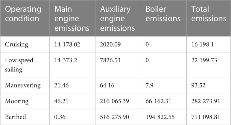
Table 1 Carbon emissions of ships under different operating conditions (t).

The primary source of air pollution in coastal and riverside ports is pollutant emissions from ships berthing at port. The high-power diesel engines on these vessels need to operate continuously to ensure the smooth functioning of onboard equipment and support systems. In normal sailing, the boiler is off. When the ship is cruising or sailing slowly, there is no load on the boiler. In many cases, therefore, the predicted carbon emissions of the boiler are 0. When the ship is cruising or sailing slowly, it is mostly in channels. When the ship is maneuvering or berthed, the ship is most likely in the anchorage or in a berth; the main engine ceases operation, and carbon emissions are generated by the auxiliary engine and boiler. A ship is berthed for about 70% of the total time it is in harbor, and the carbon emission of a berthed ship is high. When maneuvering, the ship is at low speed, and the sailing time is short; pollutant emissions are the least. Being berthed therefore drives pollutant emissions by contributing most of a ship’s total pollutant output. The carbon emission rate near the harbor anchorage and berths is significantly greater than the emission rate of other pollutants.

The reduction of ship CO₂ emissions can be accomplished through operational measures, such as reducing speed, or technical solutions like waste heat recovery (Wang et al., 2010). The cost-effectiveness and CO₂ reduction potential of each option significantly vary depending on the vessel’s type, size, and age. For instance, container ships, in contrast to oil tankers and bulk carriers, possess a greater potential for reducing emissions via speed reduction, as they are relatively slower vessels (Wang et al., 2010). Experimental studies indicate that reduced sailing speed is a pivotal measure in lowering CO₂ emissions. A speed reduction of approximately 30% in medium-sized containers can result in a fuel consumption reduction of 55% (Cariou, 2011). For the effective implementation of environmental protection and emission reduction measures, governments can utilize various policies and tools to motivate and negotiate with ports, and foster participation in carbon reduction efforts from all parties. Meanwhile, the reasonable development of environmental protection facilities such as SP, which can enhance air quality by shutting down ship diesel engines. This approach demands investments from both the port and the ship, encompassing the construction of SP facilities at the port and the upgrading of ship power facilities. Additionally, the appropriate carbon pricing signal can achieve significant results (Jiao and Wang, 2021).

3.4 Temporal fusion transformer prediction model

Taking the Tianjin Port waterway as an example, the temporal fusion transformer model with attention mechanisms was used (Lim et al., 2021). We used the high-resolution CO₂ emissions inventory of all shipping lanes in Tianjin Port as the input to the model to predict multi-horizon characteristics of carbon emissions from ships in Tianjin Port. The input contained all time-varying data and static metadata related to the target value. The equipment ID in the emissions inventory was used as the static variable, while the carbon emissions in each equipment of Tianjin Port in 2018 (with a granularity of day), year, month, day, week and day from the commencement of the study were the time-varying variables. The time series prediction model based on the attention mechanism was used to explore the characteristic relationships between the input variables and the target predictions (ship carbon emissions) to generate the range of possible target values within each forecast range. The input dataset contained emission data for 7 channels of Tianjin Port in 2018. We took days as the time step, and there were 365 time steps in the dataset. A total of 2556 time series data records were extracted and divided into a training set used for learning, with a validation set used for hyperparameter optimization and a test set used to assess the performance of the model according to the ratio of 7:2:1. Hyperparameter optimization utilized random searching. Due to the small dataset, 240 iterations were set. The epoch of each iteration was 100. The full search range for all hyperparameters was:

Hidden Layer size: 10, 20, 40, 80, 160, 240, and 320;

Dropout rate: 0.1, 0.2, 0.3, 0.4, 0.5, 0.7, and 0.9;

Minibatch size: 64, 128, and 256;

Learning rate: 0.0001, 0.001, and 0.01;

Maximum gradient norm: 0.01, 1.0, and 100.0;

Number of heads: 1 and 4.

We used the data from the previous 30 days to predict ship pollutant emissions for the next day. For model training and hyperparameter optimization, TFT was assessed by jointly minimizing quantile losses summed across all quantile outputs:

$\begin{array}{ll}ℒ(\text{Ω},W)={\sum }_{y_t\in \text{Ω}}{\sum }_{q\in Q}{\sum }_{\tau =1}^{{\tau }_{max}}\frac{QL(y_t,\widehat{y}(q,t-\tau ,\tau ),q)}{M{\tau }_{max}}& (16)\end{array}$

$\begin{array}{ll}QL(y,\widehat{y},q)=q{(y-\widehat{y})}_{+}+(1-q){(\widehat{y}-y)}_{+}& (17)\end{array}$

where Ω is the field containing the training data of M samples, W is the weight of TFT, and Q is the set of output quantiles (Q = {0.1, 0.5, 0.9} used in the experiment, and (.)₊ = max(0,.). The results of different parameters are different. The result show that the parameter configuration with Hidden Layer size = 10, Dropout rate = 0.3, Minibatch size = 128, Learning rate = 0.001, Max gradient norm = 0.01, Number of heads = 4 was optimal, and the loss value of validation set can reach about 0.14.

For the test set, the loss of normalized quantiles was assessed across the entire forecast range, focusing on P₅₀ and P₉₀ risks:

$\begin{array}{ll}q-Risk=\frac{2{\sum }_{y_t\in \widetilde{\text{Ω}}}{\displaystyle {\sum }_{\tau =1}^{{\tau }_{max}}QL}(y_t,\tilde{y}(q,t-\tau ,\tau ),q)}{{\sum }_{y_t\in \widetilde{\text{Ω}}}{\displaystyle {\sum }_{\tau =1}^{{\tau }_{max}}\left|y_t\right|}}& (18)\end{array}$

where Ω̃ is the domain of the test samples. Under optimal parameter configuration, P₅₀ and P₉₀ of the test set were approximately 0.244 and 0.118, achieving better results than the experimental data set in the paper on the TFT model (Lim et al., 2021). The predicted value of the test set and the carbon emissions in the emissions inventory are shown in Figure 9.

To further investigate how model parameters affect prediction performance, we conducted experiments on different network configurations. The performance comparison of different parameters is partially shown in Table 2.

TABLE 2

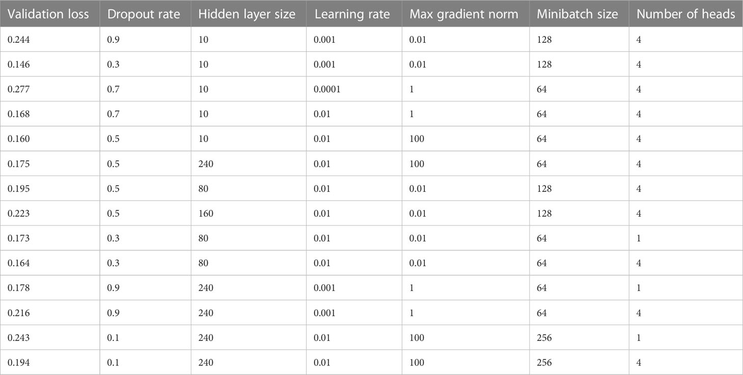
Table 2 The performance of different model parameters.

Table 2 shows that the model’s performance varied greatly under different parameters. For example, validation loss varied by as much as 0.1 with dropout rate values of 0.9 and 0.3 and other values being the same. When the learning rate was 0.0001 and 0.01, the difference in the validation loss was about 0.11. Therefore, it is necessary to find suitable hyperparameters for the model through iterations.

In this paper, root mean square error (RMSE) and mean absolute error (MAE) were used as evaluation indexes of the model. RMSE is the standard deviation of the prediction error, which represents the distance between the actual point and the predicted regression line. It also represents the distribution of the actual point around the predicted regression line, and the range is [0,+∞]. The larger the error, the larger the RMSE. The calculation formula is as follows.

$\begin{array}{ll}RMSE=\sqrt{\frac{1}{n}\sum _{i=1}^n{(\widehat{y_i}-y_i)}^2}& (19)\end{array}$

The range of MAE is [0,+∞], and the larger the error, the larger the MAE.

$\begin{array}{ll}MAE=\frac{1}{n}{\sum }_{i=1}^n\left|\widehat{y_i}-y_i\right|& (20)\end{array}$

These methods are widely employed to assess the accuracy of regression problems. For all indicators, the lower the value, the better the performance. In order to visually display the differences of model prediction performance of ship’s carbon emissions in each channel of Tianjin Port, we draw the comparison chart of model prediction performance of different channels under the optimal parameter configuration, as shown in Figure 10.

FIGURE 10

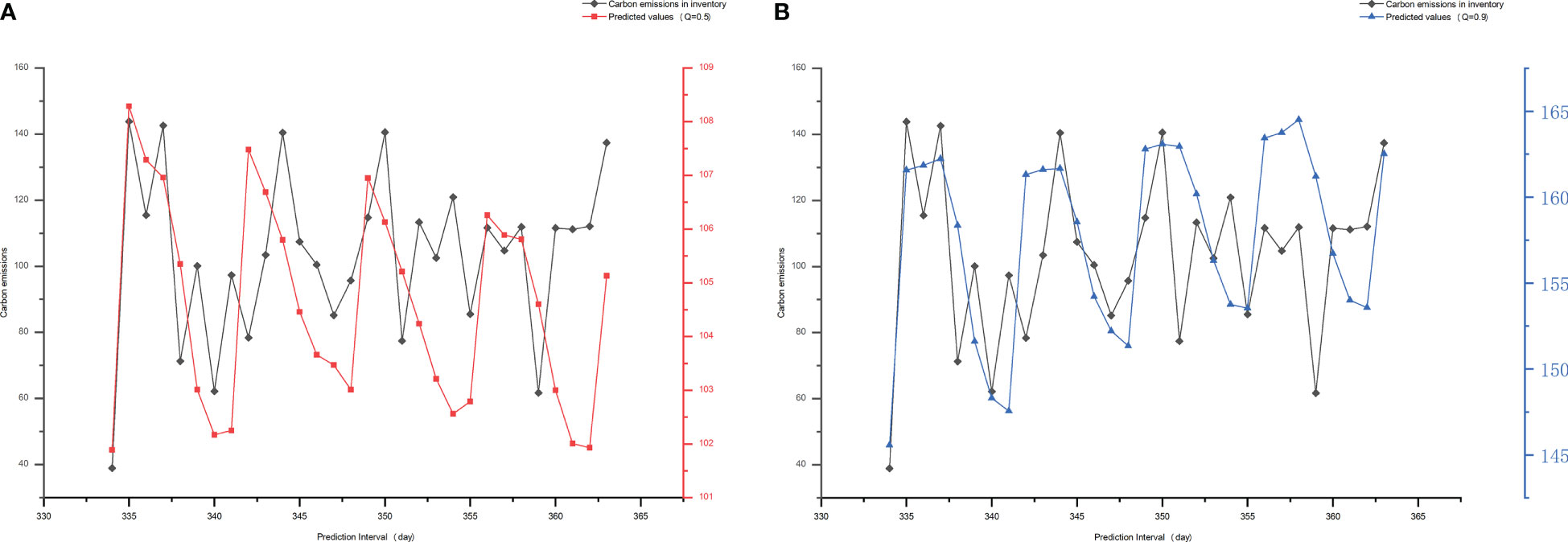
Figure 10 Prediction performance. (A) Q = 0.5; (B) Q = 0.9.

Figure 11 indicates that RMSE and MAE values under Q = 0.5 are smaller than those under Q = 0.9. Quantile Q = 0.5 indicates that there is a 50% chance that the true value will be lower than the predicted value, whereas quantile Q = 0.9 indicates that there is a 90% chance that the true value will be lower than the predicted value. Therefore, the predicted value under Q = 0.9 is higher than the real value and the predicted value under Q = 0.5, and the obtained RMSE and MAE values are also higher.

FIGURE 11

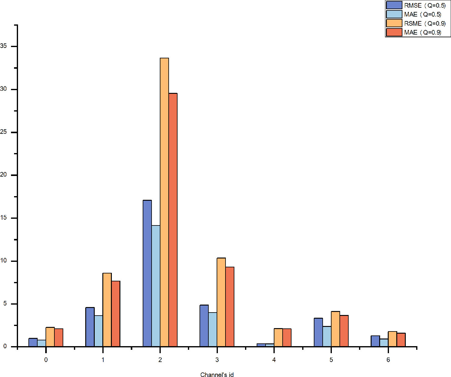
Figure 11 Comparison of model performance in different channels.

4 Discussion

Ship exhaust emissions are a primary source of air pollution in port cities. However, adopting clean energy technologies makes a ship an important protector of the inland river environment, but the extra cost of clean energy use is a barrier to its adoption by shipping enterprises. This barrier can be targeted by strict government control and policies of other relevant authorities. We used ship AIS data and Lloyd’s registry data and applied big data technologies such as data cleaning, trajectory integration, data fusion to preprocess the data to eliminate duplicate or incorrect data. We then fitted and completed missing ship information using interpolation and extrapolation to ensure high-quality accurate AIS data. The subsequent avoidance of data quality problems improved calculation results. We incorporated geographical information for Tianjin Port and dynamically calculated carbon emissions of the main engines, auxiliary engines, and boilers of ships in each channel, in berths and at anchor in Tianjin Port to create a high-resolution carbon emissions inventory of ships. We were then able to precisely trace and analyze individual ship emissions and to relate them to ship registration and vessel type. We also analyzed ship emissions from various perspectives such as space, time, ship sailing state, and emission source components. The temporal fusion transformer, a temporal prediction model based on attention mechanisms, was used to predict multi-horizon pollutant emissions of ships in Tianjin Port using high-resolution temporal ship emission data and to determine the relationships between ship operational characteristics, pollution-generating shipboard equipment, and ship carbon emissions. This study therefore provides powerful data support and theoretical reference for relevant authorities to create targeted emission reduction policies.

We used ship emission data for Tianjin Port in 2018 as an example of using the emission prediction model we employed. Time series data collected over the preceding 30 days were used to predict ship pollutant emissions for subsequent days. This high-resolution multi-feature prediction of ship carbon emissions provides pollution data that can be used as a baseline for port environmental management as it forecasts time, emission sources and emission quantities, thus making it possible for planners to respond proactively to anticipated pollution.

Sources of carbon emissions in the waterways around Tianjin Port were mainly in the vicinity of Tianjin Port, the Dagusha waterway and the main Xingang waterway. Carbon emissions peaked in July. However, in 2018, due to the fishing ban in Bohai Bay, China–United States trade disputes, and winter sea ice conditions, carbon emissions from ships in the area around Tianjin were less in some months than in other months. The government and other relevant authorities must adjust available human resources and regulatory efforts in time to respond to the high emissions in July–October and to prepare for the lifting of the fishing ban and the period of winter sea ice.

Except for ships registered to mainland China, ships registered to Hong Kong and Liberia produced most carbon emissions. This indicates that in addition to the management of China-registered vessels, control of foreign vessel emissions is necessary. Ships that illegally discharge pollutants must be dealt with seriously, but shipping companies that use clean energy can be provided with construction subsidies and carbon emission trading subsidies in the early stages of a ship’s service life to offset the cost of energy procurement and material transformation.

We analyzed pollution in terms of ship type. Dry bulk carriers produced the greatest percentage of emissions, and of other types, container ships and dry bulk carriers produced greater percentages of total pollutants than others. Tianjin Port is an international port with comprehensive cargo facilities. It has formed a cargo handling structure with containers, crude oil and related products, ore, and coal as the four pillars, and steel and grain as key cargoes. It is one of the largest comprehensive ports in the Bohai Rim region. Local governments should take advantage of the investment in capital, technology and human resources and introduce initiatives to attract more investors to promote clean energy-related projects and reach agreements with local ports and docks to prioritize the loading and unloading of clean energy ships, among other measures, to engage all parties (Xu et al., 2021).

Analysis of the operating state of vessels showed that carbon emissions were the greatest when a ship was berthed or waiting for a berth. Carbon emissions were the least when a ship was maneuvering, sailing slowly, or cruising. A ship at anchor emitted more carbon than greater than when the ship was underway. Port authorities and dock managers could optimize loading and unloading plans to reduce unnecessary emissions.

The application of a deep learning model to predicting ship pollutant emissions provides a new technique for use in emission reduction, but there remain directions for improvement in this research work. Follow-up research will continue to focus on improving the model by increasing prediction accuracy and broadening the scope of the model to provide better data for port authorities to develop proactive emission reduction policies.

Data availability statement

The authors do not have permission to share data. Requests to access these datasets should be directed to QM, meiqiang@jmu.edu.cn.

Author contributions

YL: Writing – original draft. WX: Conceptualization, methodology, writing – original draft. YY: Writing – original draft. QM: Conceptualization, writing – original draft. ZW: Data contribution. ZL: Data contribution. PW: Conceptualization. All authors contributed to the article and approved the submitted version.

Funding

This work was supported by the National Natural Science Foundation of China: [Grant Number 71804059]; Natural Science Foundation of Fujian Province: [Grant Number 2021J01821]; Shanghai Science and Technology Committee: [Grant Number 18DZ1206300]; the National Key Research and Development Program of China: [Grant Number 2018YFC1407400].

Acknowledgments

Thanks to everyone involved in the study.

Conflict of interest

The authors declare that the research was conducted in the absence of any commercial or financial relationships that could be construed as a potential conflict of interest.

Publisher’s note

All claims expressed in this article are solely those of the authors and do not necessarily represent those of their affiliated organizations, or those of the publisher, the editors and the reviewers. Any product that may be evaluated in this article, or claim that may be made by its manufacturer, is not guaranteed or endorsed by the publisher.

Supplementary material

The Supplementary Material for this article can be found online at: https://www.frontiersin.org/articles/10.3389/fmars.2023.1174411/full#supplementary-material

References

Adhikari R., Agrawal R. K. (2013). An introductory study on time series modeling and forecasting. arXiv [Preprint]. doi: 10.48550/arXiv.1302.6613

CrossRef Full Text | Google Scholar

Ammar N. R., Seddiek I. S. (2020). Enhancing energy efficiency for new generations of containerized shipping. Ocean Eng. 215, 107887. doi: 10.1016/j.oceaneng.2020.107887

CrossRef Full Text | Google Scholar

Bahdanau D., Cho K., Bengio Y. (2014). Neural machine translation by jointly learning to align and translate. arXiv [Preprint]. doi: 10.48550/arXiv.1409.0473

CrossRef Full Text | Google Scholar

Cariou P. (2011). Is slow steaming a sustainable means of reducing CO2 emissions from container shipping? Transportation Res. Part D 16 (3), 260–264. doi: 10.1016/j.trd.2010.12.005

CrossRef Full Text | Google Scholar

Chen D., Chen Y. C., Liu X. C. (2021a). Research on freight of feature mining algorithm based on multi-source water transportation big data. China Water Transport 2021 (9), 94–96. doi: 10.13646/j.cnki.42-1395/u.2021.09.035

CrossRef Full Text | Google Scholar

Chen D. S., Wang X. T., Li Y., Lang J. L., Zhou Y., Guo X. (2017). High-spatiotemporal-resolution ship emission inventory of China based on AIS data in 2014. Sci. Total Environ. 609, 776–787. doi: 10.1016/j.scitotenv.2017.07.051

PubMed Abstract | CrossRef Full Text | Google Scholar

Chen J., Xiong W., Xu L., Di Z. (2021b). Evolutionary game analysis on supply side of the implement shore-to-ship electricity. Ocean Coast. Manage. 215, 105926. doi: 10.1016/j.ocecoaman.2021.105926

CrossRef Full Text | Google Scholar

Chen J., Zhang W., Song L., Wang Y. (2022). The coupling effect between economic development and the urban ecological environment in shanghai port. Sci. Total Environ. 841, 156734. doi: 10.1016/j.scitotenv.2022.156734

PubMed Abstract | CrossRef Full Text | Google Scholar

China Knowledge Centre for Engineering Sciences and Technology (2016) Air pollutant emission inventory of marine in China. Available at: https://kgo.ckcest.cn/kgo/detail/1010/dw_reports_2020_0610/B340DC61E99259E0F60512D942782E63.html (Accessed Spetember,28,2016).

Google Scholar

Cho K., Van Merriënboer B., Gulcehre C., Bahdanau D., Bougares F., Schwenk H., et al. (2014). Learning phrase representations using RNN encoder-decoder for statistical machine translation. arXiv [Preprint]. doi: 10.48550/arXiv.1406.1078

CrossRef Full Text | Google Scholar

Clevert D.-A., Unterthiner T., Hochreiter S. (2016). Fast and accurate deep network learning by exponential linear units (ELUs). arXiv [Preprint]. doi: 10.48550/arXiv.1511.07289

CrossRef Full Text | Google Scholar

Coello J., Williams I., Hudson D. A., Kemp S. (2015). An AIS-based approach to calculate atmospheric emissions from the UK fishing fleet. Atmospheric Environ. 114, 1–7. doi: 10.1016/j.atmosenv.2015.05.011

CrossRef Full Text | Google Scholar

Connor J. T., Martin R. D., Atlas L. E. (1994). Recurrent neural networks and robust time series prediction. IEEE Trans. Neural Networks 5 (2), 240–254. doi: 10.1109/72.279188

CrossRef Full Text | Google Scholar

Corbett J. J., Winebrake J. J., Green E. H., Kasibhatla P., Eyring V., Lauer A. (2007). Mortality from ship emissions: a global assessment. Environ. Sci. Technol. 41 (24), 8512–8518. doi: 10.1021/es071686z

PubMed Abstract | CrossRef Full Text | Google Scholar

Cui J. R. (2010). The overall plan of tianjin port to create a layout of “one port and nine districts”. Port Sci. Technol. 2010 (09), 47–48. doi: CNKI:SUN:GKKJ.0.2010-09-020

Google Scholar

Dai Z., Yang Z., Yang Y., Carbonell J., Le Q. V., Salakhutdinov R. (2019). Transformer-xl: attentive language models beyond a fixed-length context. arXiv [Preprint]. doi: 10.48550/arXiv.1901.02860

CrossRef Full Text | Google Scholar

Das R., Middya A. I., Roy S. (2022). High granular and short term time series forecasting of PM 2.5 air pollutant-a comparative review. Artif. Intell. Rev. 55 (2), 1253–1287. doi: 10.1007/S10462-021-09991-1

CrossRef Full Text | Google Scholar

Devlin J., Chang M. W., Lee K., Toutanova K. (2018). Bert: Pre-training of deep bidirectional transformers for language understanding. arXiv [Preprint]. doi: 10.48550/arXiv.1810.04805

CrossRef Full Text | Google Scholar

Fan C., Huang H., Zhang Y., Pan Y., Li X., Zhang C. (2019). “Multi-horizon time series forecasting with temporal attention learning,” in Proceedings of the 25th ACM SIGKDD International Conference on Knowledge Discovery & Data Mining - KDD ‘19 (New York, NY, USA: Association for Computing Machinery). doi: 10.1145/3292500.3330662

CrossRef Full Text | Google Scholar

Feng J. C., Liu H., An F. L. (2022). Research on ship route analysis based on AIS data. Ship electronic Eng. 42 (9), 54–57 + 115. doi: 10.3969/j.issn.1672-9730.2022.09.012

CrossRef Full Text | Google Scholar

Gardner E. S. Jr. (1985). Exponential smoothing: the state of the art. J. forecasting 4 (1), 1–28. doi: 10.1002/for.3980040103

CrossRef Full Text | Google Scholar

Gers F. A., Eck D., Schmidhuber J. (2002). “Applying LSTM to time series predictable through time-window approaches,” in Neural nets WIRN vietri-01 (London: Springer), 193–200. doi: 10.1007/978-1-4471-0219-9_20

CrossRef Full Text | Google Scholar

Geurts M., Box G. E. P., Jenkins G. M. (1977). Time series analysis: forecasting and control. J. Marketing Res. 14 (2), 269. doi: 10.2307/3150485

CrossRef Full Text | Google Scholar

He L. L., Jiao Y. Q., Jia R., Liang Y. (2021). Review on the research status of air pollutant emission in port area in the development of green port. J. Chongqing Jiaotong University (Nat. Sci.) 40 (08), 78–87. doi: 10.3969/j.issn.1674-0696.2021.08.11

CrossRef Full Text | Google Scholar

Healy R. M., O’Connor I. P., Hellebust S., Allanic A., Sodeau J. R., Wenger J. C. (2009). Characterisation of single particles from in-port ship emissions. Atmospheric Environ. 43 (40), 6408–6414. doi: 10.1016/j.atmosenv.2009.07.039

CrossRef Full Text | Google Scholar

International Ship Network (2021) The latest ranking of the world’s top ten shipowners. Available at: http://www.eworldship.com/html/2021/ship_market_observation_0221/168255.html (Accessed january 27, 2020).

Google Scholar

IPCC. (2007). Climate change 2007: synthesis report. Available at: https://www.ipcc.ch/site/assets/uploads/2018/02/ar4_syr_full_report.pdf.

Google Scholar

Jiao Y., Wang C. (2021). Shore power vs low sulfur fuel oil: pricing strategies of carriers and port in a transport chain. Int. J. Low-Carbon Technol. 16 (3), 715–724. doi: 10.1093/ijlct/ctaa105

CrossRef Full Text | Google Scholar

Kim K. J. (2003). Financial time series forecasting using support vector machines. Neurocomputing 55 (1-2), 307–319. doi: 10.1016/S0925-2312(03)00372-2

CrossRef Full Text | Google Scholar

Lara-Benítez P., Carranza-García M., Riquelme J. C. (2021). An experimental review on deep learning architectures for time series forecasting. Int. J. Neural Syst. 31 (03), 2130001. doi: 10.1142/S0129065721300011

PubMed Abstract | CrossRef Full Text | Google Scholar

Lei Ba J., Kiros J. R., Hinton G. E. (2016). Layer normalization. arXiv [Preprint]. doi: 10.48550/arXiv.1607.06450

CrossRef Full Text | Google Scholar

Li C., Borken-Kleefeld J., Zheng J., Yuan Z., Ou J., Li Y. (2018). Decadal evolution of ship emissions in China from 2004 to 2013 by using an integrated AIS-based approach and projection to 2040. Atmospheric Chem. Phys. 18 (8), 6075–6093. doi: 10.5194/acp-18-6075-2018

CrossRef Full Text | Google Scholar

Li Y., Jia P., Jiang S., Li H., Kuang H., Hong Y., et al. (2023). The climate impact of high seas shipping. Natl. Sci. Rev. 10 (3), 279. doi: 10.1093/NSR/NWAC279

CrossRef Full Text | Google Scholar

Li S. Y., Jin X. Y., Xuan Y., Zhou X. Y., Chen W. H., Wang Y. X., et al. (2019). Enhancing the locality and breaking the memory bottleneck of transformer on time series forecasting. arXiv [Preprint]. doi: 10.48550/arXiv.1907.00235

CrossRef Full Text | Google Scholar

Li C., Yuan Z. B., Ou J. M., Fan X. L., Ye S. Q., Xiao T., et al. (2016). An AIS-based high-resolution ship emission inventory and its uncertainty in pearl river delta region, China. Sci. Total Environ. 573, 1–10. doi: 10.1016/j.scitotenv.2016.07.219

PubMed Abstract | CrossRef Full Text | Google Scholar

Lim B., Arık S. Ö., Loeff N., Pfister T. (2021). Temporal fusion transformers for interpretable multi-horizon time series forecasting. Int. J. Forecasting 37 (4), 1748–1764. doi: 10.1016/j.ijforecast.2021.03.012

CrossRef Full Text | Google Scholar

Liu H., Fu M. L., Jin X. X., Shang Y., Shindell D., Faluvegi G., et al. (2016). Health and climate impacts of ocean-going vessels in East Asia. Nat. Climate Change 6 (11), 1037–1041. doi: 10.1038/nclimate3083

CrossRef Full Text | Google Scholar

Liu Z. M., Lu X. H., Feng J. L., Fan Q. Z., Zhang Y., Yang X. (2017). Influence of ship emissions on urban air quality: a comprehensive study using highly time-resolved online measurements and numerical simulation in shanghai. Environ. Sci. Technol. 51 (1), 201–211. doi: 10.1021/acs.est.6b03834

CrossRef Full Text | Google Scholar

Liu H., Meng Z. H., Lv Z. F., Wang X. T., Deng F. Y., Liu Y., et al. (2019). Emissions and health impacts from global shipping embodied in US–China bilateral trade. Nat. Sustainability 2 (11), 1027–1033. doi: 10.1038/s41893-019-0414-z

CrossRef Full Text | Google Scholar

Lyu J. H., Fu F., Zuo H., Li S. F., He H. (2019). Ship emission inventory and its application in qingdao. Environ. Prot. Sci. 45 (5), 107–115. doi: 10.16803/j.cnki.issn.1004-6216.2019.05.019

CrossRef Full Text | Google Scholar

Meng L., Wang J., Yan W., Han C. (2022). A differential game model for emission reduction decisions between ports and shipping enterprises considering environmental regulations. Ocean Coast. Manage. 225, 106221. doi: 10.1016/j.ocecoaman.2022.106221

CrossRef Full Text | Google Scholar

Moldanová J., Fridell E., Popovicheva O., Demirdjian B., Tishkova V., Faccinetto A. (2009). Characterisation of particulate matter and gaseous emissions from a large ship diesel engine. Atmospheric Environ. 43 (16), 2632–2641. doi: 10.1016/j.atmosenv.2009.02.008

CrossRef Full Text | Google Scholar

Mou J. M., Zhang X. S., Yao X., Li M. X. (2019). Emission inventory of ship based on navigation data in Arctic region. J. Traffic Transportation Eng. 19 (05), 116–124. doi: 10.19818/j.cnki.1671-1637.2019.05.012

CrossRef Full Text | Google Scholar

Ng S. K. W., Loh C., Lin C., Booth V., Chan J. W. M., Yip A. C. K., et al. (2013). Policy change driven by an AIS-assisted marine emission inventory in Hong Kong and the pearl river delta. Atmospheric Environ. 76, 102–112. doi: 10.1016/j.atmosenv.2012.07.070

CrossRef Full Text | Google Scholar

Niu F. B. (2022). On the coordinated development of port logistics and regional economy–a case study of tianjin port. J. Heze Univ. 44 (04), 18–22 + 63. doi: 10.16393/j.cnki.37-1436/z.2022.04.013

CrossRef Full Text | Google Scholar

Ouyang T., Guo Y., Liu W., Zeng H. L. (2015). The job summary of international maritime organization in 2014. Shipbuilding Standardization Qual. 2015 (01), 41–45. doi: JournalArticle/5b3b7b02c095d70f0077f0f1

Google Scholar

Pan Q., Liu L. D., Ma J. W., Ma R. F. (2022). Progress in remote sensing satellite monitoring of marine environmental pollution by human activities. Mar. Sci. Bull. 41 (6), 722–736. doi: 10.11840/j.issn.1001-6392.2022.06.011

CrossRef Full Text | Google Scholar

Rehmatulla N. (2014). Market failures and barriers affecting energy efficient operations in shipping (London: UCL Energy Institute, Uni- versity College London (UCL). unpublished PhD thesis.

Google Scholar

Rehmatulla N., Smith T. (2015). Barriers to energy efficient and low carbon shipping. Ocean Eng. 110, 102–112. doi: 10.1016/j.oceaneng.2015.09.030

CrossRef Full Text | Google Scholar

Shen Z., Zhang Y., Lu J., Xu J., Xiao G. (2020). A novel time series forecasting model with deep learning. Neurocomputing 396, 302–313. doi: 10.1016/j.neucom.2018.12.084

CrossRef Full Text | Google Scholar

Shu Y. Q., Wang X. Y., Huang Z. Q., Song L., Fei Z. Q., Gan L. X., et al. (2022). Estimating spatiotemporal distribution of wastewater generated by ships in coastal areas. Ocean Coast. Manage. 222, 106133. doi: 10.1016/j.ocecoaman.2022.106133

CrossRef Full Text | Google Scholar

The Central People’s Government of the People’s Republic of China (2021) Government work report of the fourth session of the 13th national people’s congress of the people’s republic of China. Available at: http://www.gov.cn/guowuyuan/zfgzbg.html (Accessed March, 5, 2020).

Google Scholar

Thissen U. V. B. R., Van Brakel R., De Weijer A. P., Melssen W. J., Buydens L. M. C. (2003). Using support vector machines for time series prediction. Chemometrics intelligent Lab. Syst. 69 (1-2), 35–49. doi: 10.1016/S0169-7439(03)00111-4

CrossRef Full Text | Google Scholar

Tianjing Customs District P.R.China (2019) Imports of soybean at tianjin port decreased in 2018. Available at: http://tianjin.customs.gov.cn/tianjin_customs/427875/427909/427910/2280983/index.html (Accessed December 22,2022).

Google Scholar

Tianjing Municipal Bureau of Planning and Natural Resources (2017) Forecast of ice situation in tianjin from November 2017 to march 2018. Available at: https://ghhzrzy.tj.gov.cn/ztzl_143/ybyj/hbyb/202012/t20201206_4589384.html (Accessed December 22,2022).

Google Scholar

Tianjing Municipal Bureau of Planning and Natural Resources (2018) Tianjin coastal ice forecast in late February 2018. Available at: https://ghhzrzy.tj.gov.cn/ztzl_143/ybyj/hbyb/202012/t20201206_4589382.html (Accessed December 22,2022).

Google Scholar

Trozzi C. (2010) Emission estimate methodology for maritime navigation. US EPA 19th international emissions inventory conference. Available at: https://www.researchgate.net/publication/233387511_Emission_estimate_methodology_for_maritime_navigation (Accessed December 22, 2022).

Google Scholar

Vaswani A., Shazeer N., Parmar N., Uszkoreit J., Jones L., Gomez A. N., et al. (2017). Attention is all you need. arXiv [Preprint]. doi: 10.48550/arXiv.1706.03762

CrossRef Full Text | Google Scholar

Walsh C., Bows A. (2012). Size matters: exploring the importance of vessel characteristics to inform estimates of shipping emissions. Appl. Energy 98, 128–137. doi: 10.1016/j.apenergy.2012.03.015

CrossRef Full Text | Google Scholar

Wan Z., El Makhloufi A., Chen Y., Tang J. (2018). Decarbonizing the international shipping industry: solutions and policy recommendations. Mar. pollut. Bull. 126, 428–435. doi: 10.1016/j.marpolbul.2017.11.064

PubMed Abstract | CrossRef Full Text | Google Scholar

Wang R. B. (2022). A new path for tianjin port to build a world-class smart port. Construction Enterprise Manage. 2022 (08), 108–110.

Google Scholar

Wang H., Faber J., Nelissen D., Russel B., St Amand D. (2010) Reduction of GHG emissions from ships. marginal abatement costs and cost effectiveness of energy-efficiency measures. Available at: https://www.osti.gov/etdeweb/biblio/21360761 (Accessed May 18, 2023).

Google Scholar

Wang Y., Guo S., Dai L., Zhang Z., Hu H. (2022). Shore side electricity subsidy policy efficiency optimization: from the game theory perspective. Ocean Coast. Manage. 228, 106324. doi: 10.1016/j.ocecoaman.2022.106324

CrossRef Full Text | Google Scholar

Wang W. Y., Li X. Y. (2021). Research on global ship spatiotemporal big data processing and visualization. Ship Electronic Eng. 41 (8), 97–103. doi: 10.3969/j.issn.1672-9730.2021.08.024

CrossRef Full Text | Google Scholar

Weng J. X., Li G. R. (2019). Exploring shipping accident contributory factors using association rules. J. Transportation Saf. Secur. 11 (1), 36–57. doi: 10.1080/19439962.2017.1341440

CrossRef Full Text | Google Scholar

Weng J. X., Shi K., Gan X. F., Li G. R., Huang Z. (2019). Ship emission estimation with high spatial-temporal resolution in the Yangtze river estuary using AIS data. J. Cleaner Production 248 (C), 119297–119297. doi: 10.1016/j.jclepro.2019.119297

CrossRef Full Text | Google Scholar

Winters P. R. (1960). Forecasting sales by exponentially weighted moving averages. Manage. Sci. 6 (3), 324–342. doi: 10.1287/mnsc.6.3.324

CrossRef Full Text | Google Scholar

Wu J. H., Wu C., Liu W., Guo J. W. (2017). Automatic detection and restoration algorithm for trajectory anomalies of ship AIS. Navigation Of China 40 (01), 8–12 + 101. doi: 10.3969/j.issn.1672-9730.2021.08.024

CrossRef Full Text | Google Scholar

Xia K. Q. (2006). Analysis of sea ice in tianjin port and ice breaking countermeasures. Tianjin Navigation 2006 (01), 59–61.

Google Scholar

Xiao G., Xiao Y., Ni A., Zhang C., Zong F. (2022). Exploring influence mechanism of bikesharing on the use of public transportation–a case of shanghai. Transportation Lett. 15 (4), 269–277. doi: 10.1080/19427867.2022.2093287

CrossRef Full Text | Google Scholar

Xu L., Di Z., Chen J. (2021). Evolutionary game of inland shipping pollution control under government co-supervision. Mar. pollut. Bull. 171, 112730. doi: 10.1016/j.marpolbul.2021.112730

PubMed Abstract | CrossRef Full Text | Google Scholar

Yin J., Gentine P., Slater L., Gu L., Pokhrel Y., Hanasaki N., et al. (2023). Future socio-ecosystem productivity threatened by compound drought–heatwave events. Nat. Sustainability 6 (3), 259. doi: 10.1038/s41893-022-01024-1

CrossRef Full Text | Google Scholar

Yin J., Slater L., Gu L., Liao Z., Guo S., Gentine P. (2022). Global increases in lethal compound heat stress: hydrological drought hazards under climate change. Geophysical Res. Lett. 49 (18), e2022GL100880. doi: 10.1029/2022GL100880

CrossRef Full Text | Google Scholar

Zhang G. P. (2003). Time series forecasting using a hybrid ARIMA and neural network model. Neurocomputing 50, 159–175. doi: 10.1016/S0925-2312(01)00702-0

CrossRef Full Text | Google Scholar

Zhang G. P., Berardi V. L. (2001). Time series forecasting with neural network ensembles: an application for exchange rate prediction. J. operational Res. Soc. 52 (6), 652–664. doi: 10.1057/palgrave.jors.2601133

CrossRef Full Text | Google Scholar

Zhang G., Patuwo B. E., Hu M. Y. (1998). Forecasting with artificial neural networks: the state of the art. Int. J. forecasting 14 (1), 35–62. doi: 10.1016/S0169-2070(97)00044-7

CrossRef Full Text | Google Scholar

Zhang J. C., Yan S. J. (2019). Review in 2018 and outlook in 2019 of dry bulk cargo transportation market. World Shipping 42 (05), 1–9. doi: 10.16176/j.cnki.21-1284.2019.05.001

CrossRef Full Text | Google Scholar

Zhao Z. Y., Gao L., Zuo J. (2019). How national policies facilitate low carbon city development: a China study. J. Cleaner Production 234, 743–754. doi: 10.1016/j.jclepro.2019.06.116

CrossRef Full Text | Google Scholar

Zhao X., Liu L., Di Z., Xu L. (2021). Subsidy or punishment: an analysis of evolutionary game on implementing shore-side electricity. Regional Stud. Mar. Sci. 48, 102010. doi: 10.1016/J.RSMA.2021.102010

CrossRef Full Text | Google Scholar

Zhong H., Guo C., Yip T. L., Gu Y. (2021). Bi-perspective sulfur abatement options to mitigate coastal shipping ships emissions: a case study of Chinese coastal zone. Ocean Coast. Manage. 209, 105658. doi: 10.1016/J.OCECOAMAN.2021.105658

CrossRef Full Text | Google Scholar

Zhou C., Huang H., Liu Z., Ding Y., Xiao J., Shu Y. (2023). Identification and analysis of ship carbon emission hotspots based on data field theory: a case study in wuhan port. Ocean Coast. Manage. 235, 106479. doi: 10.1016/J.OCECOAMAN.2023.106479

CrossRef Full Text | Google Scholar

Zhou X., Leng Y. (2021). The challenges and countermeasures of developing zero-emission shipping. J. Shanghai Ship Shipping Res. Institute 44 (04), 63–68 + 83.

Google Scholar