Global trends in surface eddy mixing from satellite altimetry

Mixing induced by oceanic mesoscale eddies can affect tracer distributions in the ocean and thus modulate the evolution of the physical and biochemical marine system. In the context of global warming, regionally different trends in eddy mixing could exist. Motivated by this hypothesis, we quantified the trend in surface eddy diffusivity, a metric widely used to quantify the eddy mixing rate, in the global ocean using satellite altimetry data. The global average of the particle-based eddy diffusivity increases by 284.1 ${\text{m}}^2{\text{s}}^{-1}$ per decade during the period of 1994-2017, or 3.7% per decade relative to its climatological mean value. In 54% of the global ocean, eddy diffusivity shows an increasing trend. The diffusivity trend can be decomposed into two components: one related to changes in eddy mixing length and the other related to eddy velocity magnitude. In 73% of the global ocean, changes in eddy mixing length account for more than 50% of the diffusivity trend. The suppressed mixing length theory (SMLT) is employed to interpret the trend in eddy mixing length. SMLT well captures the sign of the trend in two of the representative regions. Among all the parameters (e.g., eddy size, phase speed) inherent in SMLT, the eddy velocity magnitude plays a dominant role in determining the trend in the SMLT-based eddy mixing length. Diagnosing the geostrophic eddy kinetic energy budget reveals that the dominant mechanism for the trend in eddy velocity magnitude is the pressure work induced by ageostrophic flows. Our results suggest that a time-dependent eddy parameterization scheme should be employed in non-eddy-resolving models to account for the trend in eddy mixing.

1 Introduction

Mesoscale eddies, ubiquitous in the global ocean, contain about 90% of the ocean’s kinetic energy (Ferrari and Wunsch, 2009). Eddy mixing influences the distribution of heat, salinity, and nutrients, and thus play an important role in modulating the variability of the climate system and marine ecosystem (Stammer, 1998; Gnanadesikan et al., 2015). The effect of eddy mixing is often parameterized in non-eddy-resolving climate models. Reasonable choice of eddy parameterization schemes is crucial for the realism of model simulation (Fox-Kemper et al., 2019). When implementing eddy parameterization schemes, a steady eddy diffusivity coefficient is often used (Gent and Mcwilliams, 1990; Griffies, 1998; Abernathey et al., 2011; Sun et al., 2021). However, in the context of global warming, significant trends have been found in ocean temperature and salinity, sea level, upper-ocean stratification, eddy kinetic energy (EKE) and ocean circulation (Church et al., 2011; Du et al., 2015; Hogg et al., 2015; Nan et al., 2015; Steinkamp and Gruber, 2015; Beal and Elipot, 2016; Landschützer et al., 2016; Patara et al., 2016; Syst et al., 2018; Yamaguchi and Suga, 2019; Johnson and Lyman, 2020; Martínez-Moreno et al., 2021; Beech et al., 2022; Lee et al., 2022; Peng et al., 2022; Risaro et al., 2022). It remains unclear whether a trend in oceanic mesoscale eddy mixing exists in the context of this climate change. Failure to consider this potential trend in eddy diffusivity may increase the uncertainty of climate simulations. Because climate model results are sensitive to the choice of eddy diffusivity (Danabasoglu and Marshall, 2007; Gnanadesikan et al., 2015). Therefore, this study aims to estimate and interpret the long-term trend of global surface cross-stream eddy diffusivities, which represent eddy mixing rate in the cross-mean flow direction.

Previous studies have shown that eddy diffusivity has significant spatiotemporal variability (e.g., Abernathey and Marshall, 2013; Chen et al., 2014b; Griesel et al., 2014; Busecke et al., 2017; Bolton et al., 2019; Guan et al., 2022). For example, Busecke and Abernathey (2019) found eddy mixing is linked with large-scale climate variability (e.g., El Niño-Southern Oscillation). However, few studies have provided quantitative estimates of the long-term changes in global surface cross-stream diffusivity. On the other hand, much evidence exists about the long-term trend in EKE and ocean circulation (Hogg et al., 2015; Beal and Elipot, 2016; Patara et al., 2016; Hu et al., 2020; Martínez-Moreno et al., 2021; Beech et al., 2022; Peng et al., 2022). Based on the mixing length theory and the suppressed mixing length theory (SMLT), both EKE and ocean circulation influence eddy diffusivity. Therefore, we propose that eddy diffusivity also has a significant trend in the global ocean. Specifically, the mixing length theory indicates that the eddy diffusivity is proportional to the product of eddy mixing length and eddy velocity magnitude (Taylor, 1915). Based on SMLT from Ferrari and Nikurashin (2010), cross-stream eddy mixing length is linked with eddy and mean flow properties (e.g., eddy size, phase speed, and eddy velocity magnitude).

To verify our hypothesis that eddy diffusivity has a significant trend in the global ocean, we need to estimate the global trend in surface eddy mixing. Specifically, using the Lagrangian particle approach, we first estimate the cross-stream eddy diffusivities in each year from the altimeter data. Then we estimate the trend in eddy diffusivity using the Theil-Sen estimator method (Theil, 1950; Sen, 1968). The Lagrangian particle method has been demonstrated to be effective in providing realistic and converged eddy diffusivity (e.g., Lumpkin and Elipot, 2010; Rypina et al., 2012; Chen et al., 2014b; Chen et al., 2017; Guan et al., 2022). We chose to use altimeter data because it has been proven effective in capturing the trends in ocean state (e.g., Lee et al., 2022; Peng et al., 2022).

Besides estimating mixing trends, we also aim to discuss the underlying mechanism of the trend in eddy mixing. This effort may shed light on the development of the long-term mixing trend parameterization. Using a trend decomposition method from Guo et al. (2022), we decompose the diffusivity trend into two components: One related to eddy velocity magnitude, and the other related to eddy mixing length. This decomposition can help quantify the respective contribution of eddy velocity magnitude and eddy mixing length to the diffusivity trend. We then discuss the mechanism modulating the trends in eddy velocity magnitude and eddy mixing length. For the former, we employ a novel budget of geostrophic kinetic energy. For the latter, we test the validity of SMLT in representing the trend of cross-stream eddy mixing lengths (Ferrari and Nikurashin, 2010). SMLT is capable of capturing the sign of eddy mixing trend in only two of the total five regions we consider. The origin of the trend in SMLT-based eddy mixing length is also discussed through trend decomposition.

To summarize, we aim to estimate the trend in global surface eddy diffusivity and explore the underlying mechanisms. This paper is organized as follows. Section 2 describes the dataset and presents the method for mixing and trend estimation. In section 3, we describe the trends in global surface cross-stream eddy diffusivity from both the global and regional perspectives. The respective contribution of eddy mixing length and eddy velocity magnitude to the mixing trend is quantified. Sections 4 and 5 aim to interpret the trend in eddy mixing length using SMLT. Section 4 introduces the decomposition method of the SMLT-based eddy mixing lengths, whose corresponding result is presented in section 5. Section 6 discusses the underlying mechanism of the trend in eddy velocity magnitude. Section 7 is a summary.

2 Data and method

2.1 Data

2.1.1 AVISO data and numerical particles

For diffusivity estimation, we use the geostrophic velocity data from the Archival Verification and Interpretation of Satellite Oceanographic Data (AVISO, http://www.aviso.altimetry.fr/) of the French National Space Agency. The daily velocity fields we use have a spatial resolution of 0.25° and span the time period 1994-2017. This dataset has been successfully applied in previous studies about eddy diffusivity and eddy/mean flow parameters (e.g., Abernathey and Marshall, 2013; Hogg et al., 2015; Bolton et al., 2019; Martínez-Moreno et al., 2021).

Following a series of previous work, we use the Lagrangian particle approach to estimate the Lagrangian eddy diffusivity in each year (Sallee et al., 2011; Chen and Waterman, 2017; Guan et al., 2022). An offline advection approach is used to obtain the particle trajectories covering the entire globe during 1994-2017. Taking the year 1996 as an example, we deployed virtual numerical particles offline in the global region with a resolution of 0.2°. These particles were advected by the AVISO geostrophic velocity field during 1996 based on the fourth-order Runge-Kutta method. The daily particle position and velocity information is recorded. Particles that were deployed at or advected to the land points were set to be NaN. As an example, Figure 1A shows sample particle trajectories, which were randomly selected, in the global ocean during 1996. Only 0.23% of the total number of particle trajectories are shown to make these tracks visible.

FIGURE 1

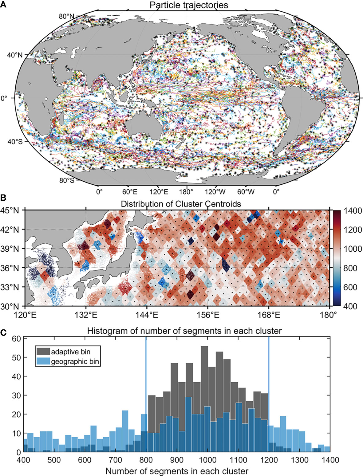
Figure 1 (A) Sample particle trajectories released on the first day of 1996. Only 0.23% of particle trajectories are randomly selected here to make these tracks visible. (B) The distribution of the centroid for each adaptive bin (black dots) in the region located at 30°N-45°N 120°E-180° of 1996. The color indicates the number of pseudo-trajectories in each adaptive bin. (C) Histogram of the number of pseudo-trajectories within each adaptive bin in panel B (gray bars) and that in each 1°×1° geographic bin (blue bars). The blue lines indicate the numbers 800 and 1200.

2.1.2 OSCAR data

Based on the mixing length theory, the diffusivity trend inferred from the AVISO geostrophic velocity field is linked with the trend of geostrophic eddy velocity magnitude $u_{rms}$(Taylor, 1915). Here

$\begin{array}{ll}{u}_{rms}=\sqrt{u_g^{\text{'}2}+v_g^{\text{'}2}}=\sqrt{2EKE},& (1)\end{array}$

where ${.}^{\prime }$ is the deviation of the daily geostrophic velocity from the annual mean, and the subscript $g$ represents the geostrophic flow. To interpret the trend of $u_{rms}$, we diagnose the geostrophic EKE budget for each year (for details of the budgetequation, see Supplementary Material 2). Considering that the ocean system is nonlinear, and geostrophic motions are coupled with ageostrophic ones, the information about both geostrophic and ageostrophic velocities is needed to diagnose the geostrophic EKE budget.

To obtain the ageostrophic velocity field, we chose to use the widely used surface velocity product: the Ocean Surface Current Analyses Real-time dataset (OSCAR). For details of OSCAR, see Bonjean and Lagerloef (2002) and Dohan (2017). The area covered by OSCAR has expanded from the equatorial region (Lagerloef et al., 1999) to the entire globe, providing daily surface currents velocity on a global 0.25°× 0.25° grid. Consistent with AVISO, we chooseto use the OSCAR data during the period 1994-2017.

The surface total velocity from OSCAR is calculated from a simplified physical model,

$\begin{array}{ll}\text{f}\text{k}\times {\text{U}}_{\text{o}}=-\frac{1}{\rho }\nabla p+\frac{1}{\rho }\frac{\partial \tau }{\partial z},& (2)\end{array}$

where $f$ is Coriolis parameter, $U_o=u_{o}i+v_{o}j$, representing total velocity from OSCAR, $\rho$ is the sea surface density, $p$ is the sea surface pressure, and $\tau$ is the surface wind stress. Satellite-observed datasets including sea surface height gradients, ocean vector winds and sea surface temperature gradients were used to produce the OSCAR dataset. Equation (2) shows that this model contains geostrophic, Ekman, and thermal wind dynamics.

Subtracting the AVISO geostrophic velocity from OSCAR total velocity ($U_o$) leads to the ageostrophic velocity. The physical model [Equation (2)] indicates that the ageostrophic flow inferred from OSCAR mainly contains the Ekman flow. Considering that this model is linear and does not capture nonlinear dynamics, other components (e.g., submesoscale ageostrophic motions) are not well captured by OSCAR. Nonetheless, much evidence has demonstrated that this dataset is useful for studies about mesoscale eddies and the EKE budget. For example, using OSCAR data, Chen et al. (2018) studied the spatial distribution and seasonal variability of EKE in the Bay of Bengal region. Piontkovski et al. (2019) investigated the interannual variability of the occurrence of mesoscale eddies in the western Arabian Sea. In addition, although surface drifter data may provide more realistic total velocity fields, its non-uniform spatiotemporal distribution make it challenging to diagnose the EKE budget at drifter points (Yu et al., 2019). Therefore, we use the OSCAR dataset to infer the ageostrophic velocity.

2.2 Method

2.2.1 Mixing estimation method

Following a series of previous studies (e.g., Chen et al., 2014b; Chen et al., 2017; Guan et al., 2022), we estimate the cross-stream eddy diffusivity using a Lagrangian autocorrelation function based on particle trajectories. This approach is generally termed as the Lagrangian particle method and have been proven effective for converged diffusivity estimates (Davis, 1987; Davis, 1991; LaCasce and Bower, 2000; Zhurbas and Oh, 2004; Lumpkin and Elipot, 2010; Rypina et al., 2012; Chen et al., 2014b; Chen et al., 2017; Guan et al., 2022). The diagnostic formula for cross-stream (i.e., cross-mean flow) eddy diffusivity is

$\begin{array}{ll}{\kappa }_{\perp ,particle}(\mathbf{\text{x}})=\underset{\tau \to \infty }{\lim }{\kappa }_{\perp }(\text{x},\tau )\approx \frac{{\int }_{{\tau }_1}^{{\tau }_2}{\kappa }_{\perp }(\mathbf{\text{x}},\tilde{\tau })d\tilde{\tau }}{{\tau }_2-{\tau }_1},& (3)\end{array}$

where

$\begin{array}{ll}{\kappa }_{\perp }(\mathbf{\text{x}},\tau )={\displaystyle {\int }_0^{\tau }d\tilde{\tau }{\langle u_{g\perp }^{\text{'}}(t_0|\mathbf{\text{x}},t_0)u_{g\perp }^{\text{'}}(t_0+\tilde{\tau }|\mathbf{\text{x}},t_0)\rangle }_L.}& (4)\end{array}$

Here the bracket $\langle ·\rangle$ represents the ensemble average of all the pseudo-trajectories passing the adaptive bin centered at $\text{x}$. For example, Figure 2A shows sample pseudo-trajectories through the adaptive bin centered at (167.91°E, 53.41°N). $u_{g\perp }^{\text{'}}(t_0+\tilde{\tau }|\text{x},t_0)$ represents the cross-stream geostrophic eddy velocity at time $t_0+\tilde{\tau }$ at the position of the particle, which passes the position $x$ at time $t_0$. As $\tau$ increases, the velocity gradually gets decorrelated with the initial velocity and ${\kappa }_{\perp }(\text{x},\tau )$ asymptotes to a constant value, i.e., has converged. The Lagrangian equilibration time ${\tau }_{eq}$ is the minimum time it takes for ${\kappa }_{\perp }(\text{x},\tau )$ to level off. We use the criteria from Chen and Waterman (2017) to judge whether ${\kappa }_{\perp }(\text{x},\tau )$ has leveled off. In brief, when the change rate of the fitted ${\kappa }_{\perp }(\text{x})$ over a 30-day period (i.e. $[{\tau }_1,{\tau }_2]$) is less than the minimum value of two standard errors during that period, we consider ${\kappa }_{\perp }(\text{x})$ has leveled off. Here ${\tau }_{eq}=({\tau }_{1s}+{\tau }_{2s})/2.0$, where $[{\tau }_{1s},{\tau }_{2s}]$ denotes the smallest $[{\tau }_1,{\tau }_2]$ with converged ${\kappa }_{\perp }(\text{x},\tau )$. As an example, the grey line in Figure 2B shows ${\tau }_{eq}$ in the adaptive bin centered at (167.91°E, 53.41°N).

FIGURE 2

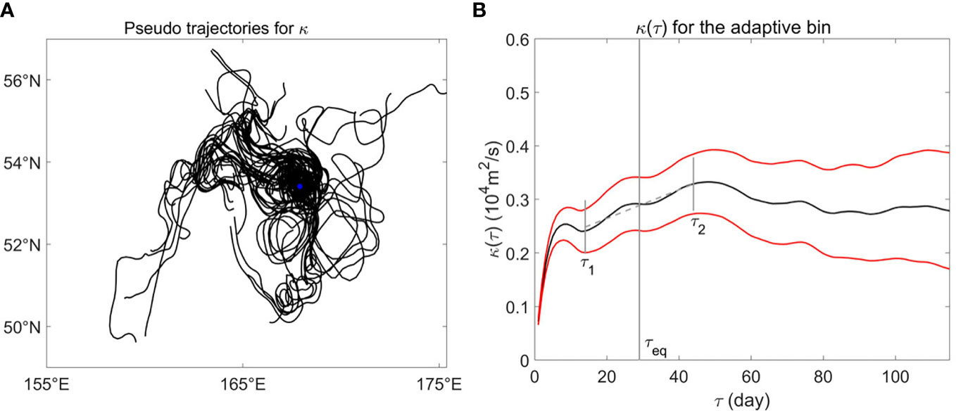
Figure 2 (A) Sample pseudo-trajectories through the adaptive bin centered at 167.91°E, 53.41°N. The blue dot shows the centroid of the adaptive bin. (B) ${\kappa }_{\perp }(\text{x},\tau )$ [Equation 4] as a function of $\tau$ in the adaptive bin from (A). Red lines show the uncertainties of ${\kappa }_{\perp }(\text{x},\tau )$ at the 95% confidence level via a bootstrapping method. The vertical grey line indicates the equilibration time ${\tau }_{eq}$, where ${\kappa }_{\perp }(\text{x},\tau )$ starts leveling off.

We chose to use pseudoparticle trajectories instead of the original particle trajectories to improve the convergence of eddy diffusivity (Chen et al., 2014b; Chen et al., 2017; Guan et al., 2022). Specifically, a point is selected every few days from the original trajectory as the initial position of the pseudo-trajectory, and a certain track length for the pseudo-trajectory is selected. It can increase the number of trajectories and make diffusivity converge (Griesel et al., 2010; Klocker et al., 2012). To ensure the convergence of eddy diffusivity, the length of pseudo-trajectories should be longer than the Lagrangian equilibrium time. Yet, the longer the pseudo-trajectory is, the smaller the number of pseudo trajectories is. And adequate amount of pseudo trajectories in each bin is a prerequisite for obtaining converged diffusivity estimates. Considering this, we choose 115 days to be the pseudo-trajectory length in this study. The interval between the adjacent initial positions of pseudo-trajectories is chosen to be five days.

To further improve the convergence of eddy diffusivity, we choose to use the adaptive-bin method based on the K-means algorithm (Koszalka and LaCasce, 2010; Chen et al., 2014b; Guan et al., 2022) instead of the geographic bin method. Due to the flow inhomogeneity, the number of pseudo-trajectories in the regular geographic bins varies greatly (Figure S1 in Supplementary Material), leading to poor convergence of diffusivity estimates. As an example, the blue bars in Figure 1C show the histogram of the number of pseudo-trajectories in each 1°×1° geographic bin in a selected region located at 30°N-45°N 120°E-180°. The histogram has a wide shape and the number of tracks ranges from 400-1400. The advantage of using adaptive bins instead of geographic bins is that the K-means algorithm can make sure the number of the tracks in each bin is roughly the same. Take the region located at 30°N-45°N 120°E-180° as an example, the adaptive bins are randomly distributed in this area (Figures 1B, C). However, the number of pseudo-trajectories in each adaptive bin is roughly uniform ranging from 800 to 1200. In this case, the average size of adaptive bins in the global ocean is roughly 1°× 1°. We find that increasing the number of pseudo-trajectories in each adaptive bin will increase the size of adaptive bins and thus decrease the spatial resolution of our eddy mixing estimates. However, the large-scale structures of eddy diffusivities is insensitive to this change.

2.2.2 Trend estimation method

We chose to use the Theil-Sen estimator (TS) approach (Theil, 1950; Sen, 1968) for trend estimation in this study. The TS method is a robust non-parametric statistical method for estimating trends. The disadvantage of the commonly used simple linear regression method is that the estimated trend is sensitive to the outliers in time series (Ohlson and Kim, 2015). In contrast, the TS method is insensitive to both the outliers and uncertainties in time series. Therefore, the TS method has been widely used in the analysis of trend in meteorological and oceanographic variables (Gocic and Trajkovic, 2013; Sa’adi et al., 2019; Zhao et al., 2022).

The statistical significance of the estimated trend is assessed through a modified Mann-Kendall test (Mann, 1945; Kendall, 1948; Hamed and Rao, 1998). This method has been widely used to determine the statistical significance of the estimated trend (Yue and Wang, 2004; Hu et al., 2020; Zhao et al., 2022). The advantage of this method is that it neither requires the time series to be in a normal distribution nor requires the trend to be linear. In addition, it is neither affected by missing values nor influenced by abnormal data points. Furthermore, this method can effectively eliminate the impact of serial correlation on the estimated trend. Thus, it can be used to assess the trend significance for the time series with autocorrelation (Hamed and Rao, 1998).

3 Trends in eddy mixing

3.1 Global analysis

3.1.1 Spatial structure

The trend of ${\kappa }_{\perp ,particle}$ in the global ocean has large spatial variability (Figure 3A). The trend magnitude is large in the western boundary currents and their extension regions, the equatorial Indian Ocean, and the central equatorial Pacific Ocean. In particular, there is a significant increase trend of ${\kappa }_{\perp ,particle}$ in the equatorial Pacific Ocean, with a magnitude as large as 5000 ${\text{m}}^2{\text{s}}^{-1}$ per decade. In the western boundary currents and their extension regions, the structure of the ${\kappa }_{\perp ,particle}$ trend is patchy. The trend is negative in the upstream of the Kuroshio Extension, but positive in the downstream. The opposite occurs at the Gulf Stream Extension, with positive (negative) trend in the upstream (downstream).

FIGURE 3

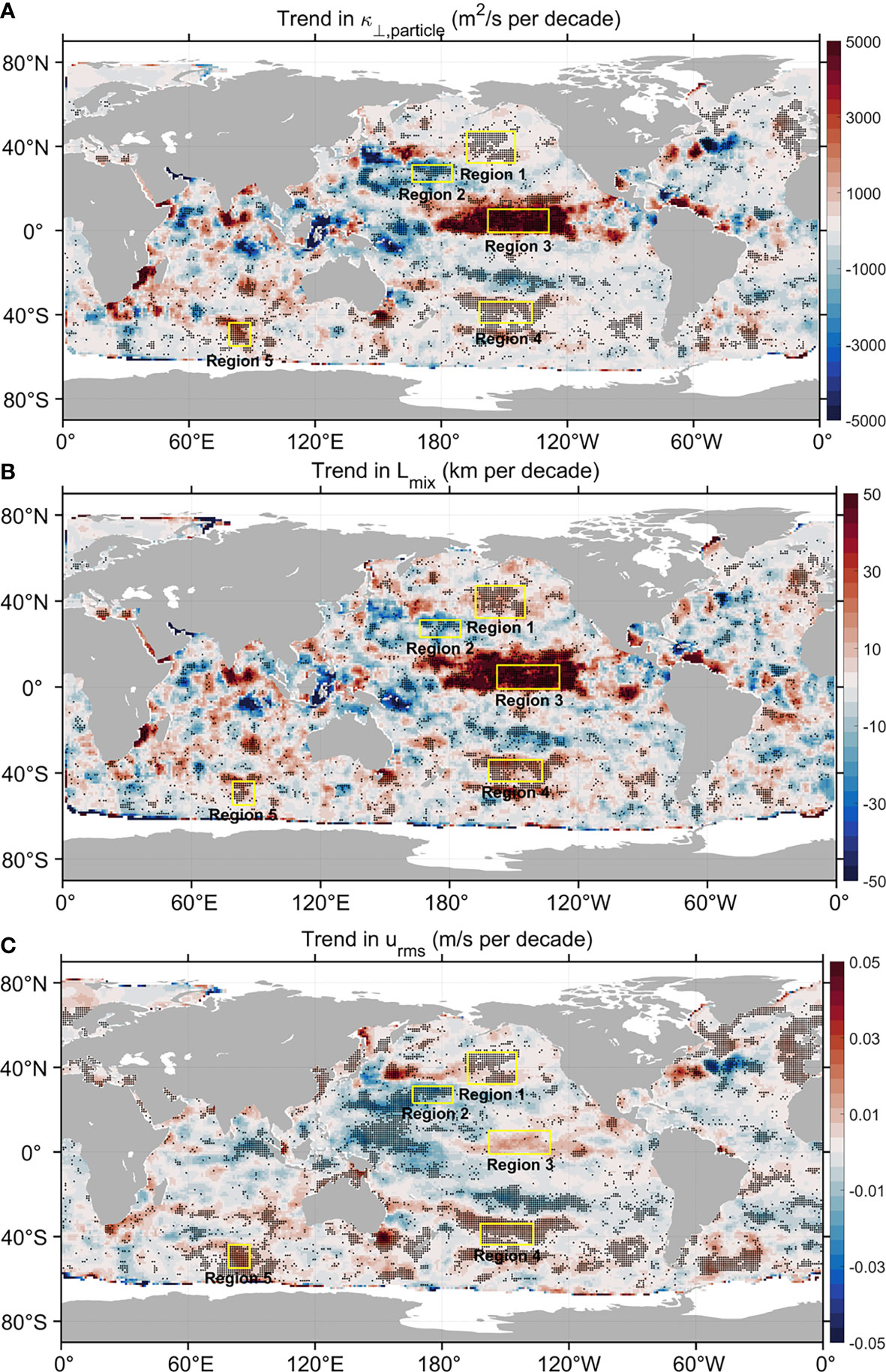
Figure 3 The trend of (A) ${\kappa }_{\perp ,particle}$, (B) $L_{mix,particle}$, and (C) $u_{rms}$ in the global ocean during the period 1994-2017. The trend diagnosis method is described in section 2.2.2. Black dots indicate the grid points, where the trend is statistically significant at the 95% confidence level. Yellow boxes show the five representative regions we discuss.

From a global perspective, the trend of the globally integrated ${\kappa }_{\perp ,particle}$, inferred from the TS method, is 284.1 ${\text{m}}^2{\text{s}}^{-1}$ per decade (Figure 4). It accounts for 3.7% of the climate-mean ${\kappa }_{\perp ,particle}$. ${\kappa }_{\perp ,particle}$ shows an increasing trend in 54% of the global ocean. Among these areas with an increasing trend, 17.7% is significant at the 95% confidence level.

FIGURE 4

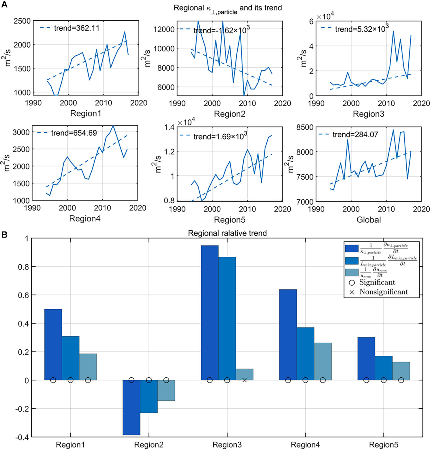
Figure 4 (A) The spatially averaged ${\kappa }_{\perp ,particle}$ time series (blue solid line) and its trend (blue dashed line, $m^2{s}^{-1}$ per decade) in both the five representative regions and the global ocean. These representative regions are indicated in Figure 3. (B) The relative trends of ${\kappa }_{\perp ,particle}$, $L_{mix,particle}$, and $u_{rms}$ [Equation (6)] in the five representative regions during 1994-2017. Statistically insignificant trends at the 95% confidence level are marked by “ $\times$“, and significant trends are marked by “ $\circ$“.

Based on the mixing length theory (Taylor, 1915), eddy diffusivity is proportional to the product of eddy mixing length and eddy velocity magnitude. Therefore, the particle-based eddy mixing length,

$L_{mix,particle}$, can be diagnosed from

$\begin{array}{ll}{L}_{mix,particle}=\frac{{\kappa }_{\perp ,particle}}{\Gamma u_{rms}}.& (5)\end{array}$

Here $u_{rms}$ is eddy velocity magnitude and $\text{Γ}$ is the mixing efficiency with magnitude of O(1). Following previous studies, we choose $\text{Γ}$ to be 0.35 (e.g., Chen et al., 2014b; Chen et al., 2017; Busecke and Abernathey, 2019; Guan et al., 2022). Equation (5) indicates that both the trend in $L_{mix,particle}$ and the trend in $u_{rms}$ contribute to the trend in ${\kappa }_{\perp ,particle}$. Positive trends in $L_{mix,particle}$ and $u_{rms}$ lead to increasing trend in ${\kappa }_{\perp ,particle}$. On the other hand, negative trends of these two factors lead to decreasing trend in ${\kappa }_{\perp ,particle}$.

Since the trend of ${\kappa }_{\perp ,particle}$ arises from the trends in $L_{mix,particle}$ and $u_{rms}$. Here we assess the global trend distributions of both $L_{mix,particle}$ and $u_{rms}$ (Figures 3B, C). Compared to the trend in $u_{rms}$, the global structure of the $L_{mix,particle}$ trend resembles more to that of the ${\kappa }_{\perp ,particle}$ trend. Similar to ${\kappa }_{\perp ,particle}$, the large magnitude of the $L_{mix,particle}$ trend occurs in the western boundary currents and their extension regions, the equatorial Indian Ocean, and the central equatorial Pacific Ocean. In contrast, the large trend in $u_{rms}$ only occurs in the western boundary currents and their extension regions. In the central equatorial Pacific Ocean, the trend of $L_{mix,particle}$ increases significantly, with a magnitude as large as 50 $\text{km}$ per decade. In contrast, the increasing trend of $u_{rms}$ is insignificant in the central equatorial Pacific Ocean.

Our analysis in Figure 5 indicates that compared to $u_{rms}$, the trend of $L_{mix,particle}$ contributes more to that of ${\kappa }_{\perp ,particle}$. The correlation coefficient of the trends between $L_{mix,particle}$ and ${\kappa }_{\perp ,particle}$ reaches 0.69. The errorbar, based on a bootstrapping technique technique (Chernick, 2011; Chen et al., 2014b; Schulte et al., 2016; Ivanova et al., 2021), is 0.02 at the 95% confidence level (Figure 5A). Concerning $u_{rms}$, its trend is also positively correlated with the ${\kappa }_{\perp ,particle}$ trend, with a weaker correlation magnitude though (0.37 $\pm$ 0.02 at the 95% confidence level) (Figure 5A). In 89% (75%) of the global ocean area the sign of the trend in $L_{mix,particle}$($u_{rms}$) is consistent with that of ${\kappa }_{\perp ,particle}$ (Figure 5B).

FIGURE 5

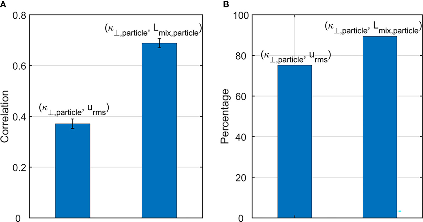
Figure 5 (A) The correlation coefficient of the global trends between ${\kappa }_{\perp ,particle}$ and $u_{rms}$, and that between ${\kappa }_{\perp ,particle}$ and $L_{mix,particle}$. The errorbar is at the 95% confidence level by the bootstrapping method. (B) The percentage of the grid points where $u_{rms}$($L_{mix,particle}$) and ${\kappa }_{\perp ,particle}$ trends have the same sign.

3.1.2 Decomposition of the mixing trend

Although the mixing length theory [Equation (5)] suggests that eddy diffusivity is proportional to eddy velocity magnitude and eddy mixing length, it remains unclear which of these two factors contributes more to the diffusivity trend. To quantify the contribution of each factor to the trend in eddy diffusivity, we introduce a metric “relative trend”. Then we employ a trend decomposition method to quantitatively decompose the relative trend of ${\kappa }_{\perp ,particle}$ into two components: One related to $L_{mix,particle}$ and the other related to $u_{rms}$ [Equation (6)].This decomposition approach is inspired by Guo et al. (2022), who successfully decomposed the trend in eddy heat flux into components related to the velocity variance, temperature variance, and coherence parameters, respectively. By taking the logarithm on both sides of Equation (5) and then computing their temporal derivatives, the relative trend of ${\kappa }_{\perp ,particle}$can be expressed as

$\begin{array}{ll}\frac{1}{{\kappa }_{\perp ,particle}}\frac{\partial {\kappa }_{\perp ,particle}}{\partial t}=\frac{1}{u_{rms}}\frac{\partial u_{rms}}{\partial t}+\frac{1}{L_{mix,particle}}\frac{\partial L_{mix,particle}}{\partial t}.& (6)\end{array}$

That is, the relative trend of ${\kappa }_{\perp ,particle}$ is equal to the sum of the relative trend in $L_{mix,particle}$ and that in $u_{rms}$. Using Equation (6), one can quantify the contribution of each factor to the relative trend of ${\kappa }_{\perp ,particle}$.

We estimated the relative trends in ${\kappa }_{\perp ,particle}$, $L_{mix,particle}$ and $u_{rms}$ in the global ocean (Figure 6). The relative trend of ${\kappa }_{\perp ,particle}$ has elevated positive values in the equatorial central Pacific and at high latitudes of the northeast Pacific and Atlantic Oceans. Its value is also significantly large around 40°S in the central Pacific. However, the relative trend in ${\kappa }_{\perp ,particle}$ is negative at 20°S-30°N in thewestern Pacific. Similar to ${\kappa }_{\perp ,particle}$, the relative trend in $L_{mix,particle}$ also has significant positive values in the central equatorial Pacific and at the high-latitude Pacific. Concerning the relative trend in $u_{rms}$, it is generally positive in the Southern Ocean and at high-latitude regions of the Northern Hemisphere. In the equatorial eastern Pacific, the relative trend of $u_{rms}$ is positive but smaller than that at high-latitudes. In contrast, the relative trend of $u_{rms}$ is negative in both the equatorial western Pacific and the mid-latitude Pacific.

FIGURE 6

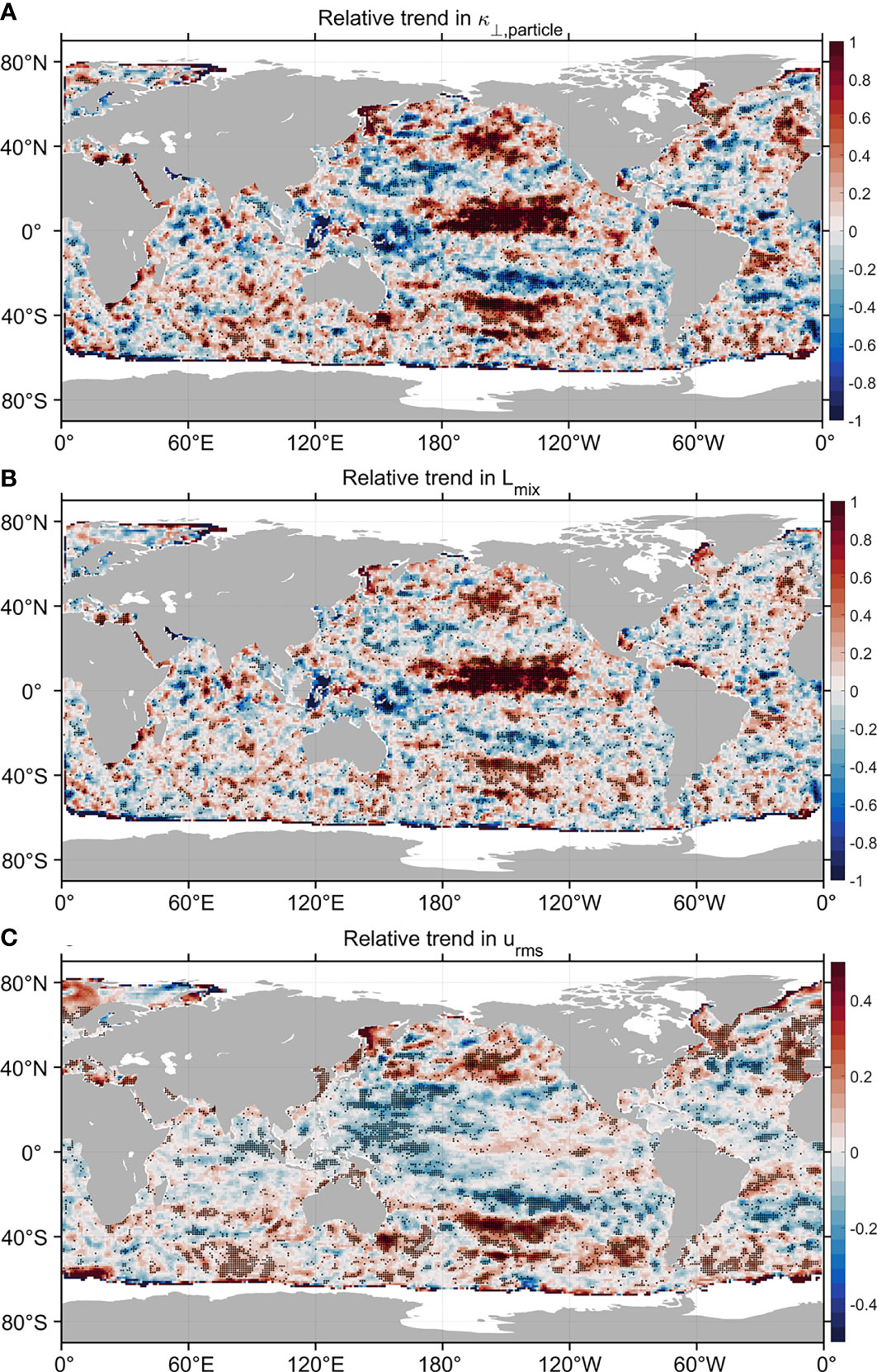
Figure 6 The relative trend of (A) ${\kappa }_{\perp ,particle}$, (B) $L_{mix,particle}$, and (C) $u_{rms}$ from Equation (6) in the global ocean during the period 1994-2017. Black dots indicate the grid points where the relative trend is statistically significant at the 95% confidence level.

To assess the respective contribution of $L_{mix,particle}$ and $u_{rms}$ to the relative trend in ${\kappa }_{\perp ,particle}$, we diagnosed the ratio of the relative trends between $L_{mix,particle}$ and ${\kappa }_{\perp ,particle}$ and that between $u_{rms}$ and ${\kappa }_{\perp ,particle}$. A positive (negative) ratio of the relative trends between $L_{mix,particle}$ and ${\kappa }_{\perp ,particle}$ indicates that $L_{mix,particle}$ has a positive (negative) effect on the relative trend of ${\kappa }_{\perp ,particle}$. We can also interpret the contribution of $u_{rms}$ to ${\kappa }_{\perp ,particle}$ in an analogous way. Our results, shown in Figures 7A and 6B, suggest that compared to $u_{rms}$, $L_{mix,particle}$ contributes much more to the relative trend in ${\kappa }_{\perp ,particle}$.

FIGURE 7

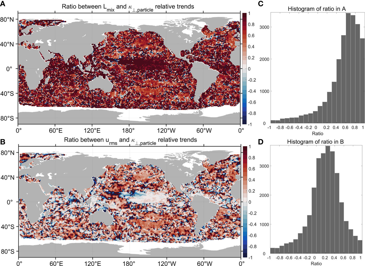
Figure 7 (A) The ratio of the relative trends between $L_{mix,particle}$ and ${\kappa }_{\perp ,particle}$ in the global ocean. (B) The ratio of the relative trends between $u_{rms}$ and ${\kappa }_{\perp ,particle}$ in the global ocean. (C) and (D) show histograms of the ratios from panels A and B.

The ratio of the relative trends between $L_{mix,particle}$ and ${\kappa }_{\perp ,particle}$ is generally larger than that between $u_{rms}$ and ${\kappa }_{\perp ,particle}$ (Figures 7A, B). In 65% (73%) of the global ocean, the ratio of the relative trends between $L_{mix,particle}$ and ${\kappa }_{\perp ,particle}$ relative trends is larger than 0.6 (0.5). We also evaluated the probability density functions (PDFs) of these ratios (Figures 7C, D). For the ratio between the $L_{mix,particle}$ and ${\kappa }_{\perp ,particle}$ relative trends, the PDF is wide and asymmetric with a skewness value of 2.73 (Figure 7C). Its peak approximately occurs at 0.6. As to the ratio between the $u_{rms}$ and ${\kappa }_{\perp ,particle}$ relative trends, its PDF is only slightly asymmetric with a skewness value of 0.47 (Figure 7D). The PDF peak approximately occurs at 0.3. Comparing the two PDFs further reveal that $L_{mix,particle}$ plays a larger role than $u_{rms}$ in modulating the relative trend of ${\kappa }_{\perp ,particle}$.

3.2 Regional analysis

Considering that the mixing trend has complex spatial variability, next we focus on five representative regions to further characterize and interpret the mixing trend in the ocean (yellow boxes in Figure 3). All these five regions have statistically significant mixing trend (Figure 4A). They respectively represent areas with large positive mixing trends (Regions 3 and 5), weak positive mixing trend (Regions 1 and 4), and large negative mixing trend (Region 2). Region 3 is located in the equatorial Central Pacific, where the largest positive mixing trend occurs. Previous studies have shown that eddy mixing in the equatorial region is linked with the large-scale climate variability (e.g., El Niño-Southern Oscillation; Gnanadesikan et al., 2017; Busecke and Abernathey, 2019). Regions 1 and 4 are located in the mid-ocean regions in the Pacific. The mixing trend in these two regions are positive but weak. Region 5 is a representative patch in the Antarctic Circumpolar Current and mixing there is relatively strong and positive. There are also regions with negative mixing trends in the global oceans, for example Region 2.

The time series of the regionally averaged ${\kappa }_{\perp ,particle}$ and the corresponding trends based on TS method are shown in Figure 4A. The trends in all the five regions are statistically significant at the 95% confidence level. In Region 2, the ${\kappa }_{\perp ,particle}$ time series has a negative trend, decreasing by 1.62 $\times$ 10³ ${\text{m}}^2{\text{s}}^{-1}$ per decade. It accounts for 18.8% of the climate mean ${\kappa }_{\perp ,particle}$. In all the other four regions, the ${\kappa }_{\perp ,particle}$ time series have positive trends. Among these four regions, the trend in Region 3 is the largest, with a magnitude of 5.32 $\times$ 10³ ${\text{m}}^2{\text{s}}^{-1}$ per decade and accounting for 31.0% of the climate mean value. These results suggest that eddy mixing effect will be significantly enhanced in the context of tropical climate change.

We also carried out the mixing trend decomposition, based on Equation (6). In all these regions, the relative trend of $L_{mix,particle}$ has magnitude larger than that of $u_{rms}$ (Figure 4B). The $L_{mix,particle}$ relative trend accounts for 56%-91% of the relative trend in ${\kappa }_{\perp ,particle}$, indicating that $L_{mix,particle}$ contributes more than $u_{rms}$ to the trend in ${\kappa }_{\perp ,particle}$. On the other hand, the relative trends of both $L_{mix,particle}$ and $u_{rms}$ are statistically significant at the 95% confidence level, except for the $u_{rms}$ trend in Region 3.

To keep this study concise and reader-friendly, we only focus on five regions with significant mixing trends, located in either the Pacific Ocean or the Southern Ocean. Note, that, there are also regions in other basins with significant mixing trends, such as 39°N-57°N 10°W-20°W in the Atlantic Ocean. In this Atlantic box, the eddy diffusivity trend is 555.5 m²s^-1 per decade. Consistent with the five regions we focus on, the $L_{mix,particle}$ relative trend in this box is also larger than that of $u_{rms}$ (not shown).

4 Suppressed mixing length theory and its trend decomposition

Since eddy mixing length and eddy velocity magnitude jointly determine eddy diffusivity [Equation (5)], separately interpreting the trends in mixing length and eddy velocity magnitude can help reveal the underlying mechanism of eddy mixing trend. We chose to use SMLT to discuss the mechanism of the trends in eddy mixing length (sections 4 and 5). In this section, we first introduce SMLT and then describe how to decompose the relative trend of SMLT-based mixing length into those of eddy and mean flow properties.

4.1 Suppressed mixing length theory

Though several mixing theories have been proposed (Ferrari and Nikurashin, 2010; Bates et al., 2014; Chen et al., 2015; Jansen et al., 2015; Wei and Wang, 2021), none of them can perfectly represent eddy mixing lengths. One of these theories that receive much attention is SMLT (Ferrari and Nikurashin, 2010), which is built on the critical layer idea from Green (1970). SMLT is derived based on several assumptions (e.g., linear, flat and homogeneous system, single-wave representation of eddies) (Ferrari and Nikurashin, 2010; Chen et al., 2015) and it often breaks down at topographic regions (Naveira Garabato et al., 2011; Chen et al., 2014b). However, it successfully represent the mixing suppression phenomenon induced by the propagation of eddies relative to the mean flow (e.g., Ferrari and Nikurashin, 2010; Klocker et al., 2012b). Much evidence shows that SMLT can well capture the large-scale spatial structure of eddy mixing (e.g., Ferrari and Nikurashin, 2010; Klocker et al., 2012b; Abernathey and Marshall, 2013; Bates et al., 2014; Klocker and Abernathey, 2014; Roach et al., 2016; Roach et al., 2018; Groeskamp et al., 2020). In addition, SMLT-based eddy mixing was found to be linked with the large-scale climate variability (Busecke and Abernathey, 2019). Since this study focuses on the large-scale and long-term variability of eddy mixing, we chose to discuss the mechanism of the eddy mixing length trend using SMLT.

In brief, SMLT explicitly expresses the cross-stream eddy mixing length as a function of mean flow and eddy properties. Based on this theory, eddy mixing length in the cross-stream direction can be written as the product of eddy size $L_{eddy}$ and a suppression factor $S$ ($\le$1),

$\begin{array}{ll}{L}_{mix,SMLT}=L_{eddy}\underset{S}{\underbrace{\left[\frac{1}{1+k_{eddy}^2{\gamma }^{-2}{(c_w-\left|U_g\right|)}^2}\right]}}.& (7)\end{array}$

Following Chen et al. (2014b), $L_{eddy}$ can be estimated from

$\begin{array}{ll}{L}_{eddy}(x,y)=2\pi \underset{k_{eddy}^{-1}(x,y)}{\underbrace{\left[\frac{{\iint }^{}{S}_{EKE}(k,l)dkdl}{{\iint }^{}\sqrt{k_2+l_2}{S}_{EKE}(k,l)dkdl}\right]}},& (8)\end{array}$

where $k_{eddy}$ refers to the dominant eddy wavenumber, $S_{EKE}(k,l)$ is the wavenumber spectra of geostrophic EKE, $k$ represents the zonal wavenumber, and $l$ denotes the meridional wavenumber. The variable $\left|{\text{U}}_g\right|$ is the magnitude of the geostrophic mean flow and $c_w$ represents the phase speed along the direction of geostrophic mean flow. Therefore, the term $c_w-\left|{\text{U}}_g\right|$ in the suppression factor $S$ represents the propagating speed of eddies relative to the mean flow. The phase speed $c_w$ is estimated from the Hovmöller diagram of sea surface height anomaly using the Radon transform method (Guan et al., 2022). As stated in Chen et al. (2014b), ${\gamma }^{-1}$ represents the eddy decorrelation time scale,

$\begin{array}{ll}\gamma (x,y)=\frac{u_{rms}(x,y)}{2\Gamma L_{eddy}(x,y)}.& (9)\end{array}$

All these parameters above are diagnosed using AVISO data.

Based on Equations (7)- (9), we can obtain another expression of SMLT,

$\begin{array}{ll}{L}_{mix,SMLT}=L_{eddy}\underset{S}{\underbrace{\left[\frac{1}{1+16{\pi }^2{\Gamma }^2{u}_{rms}^{-2}{(c_w-\left|U_g\right|)}^2}\right].}}& (10)\end{array}$

Similar to Equation (5), based on the mixing length theory (Taylor, 1915), we can diagnose the SMLT-based cross-stream eddy diffusivity from

$\begin{array}{ll}{\kappa }_{\perp ,SMLT}=\text{Γ}{u}_{rms}{L}_{mix,SMLT}.& (11)\end{array}$

4.2 Decomposition of eddy mixing length trends

Equation (10) shows that the SMLT-based eddy mixing length is mainly regulated by the following three terms: $L_{eddy}$, $u_{rms}$ and $c_w-\left|{\text{U}}_g\right|$. We can explore their respective contribution to the trend of eddy mixing length using the trend decomposition method from Guo et al. (2022). Note that this decomposition method has also been used in section 3.1.2. The SMLT-based eddy mixing length ($L_{mix,SMLT,2}$) trend can be decomposed as follows:

$\begin{array}{ll}\frac{1}{L_{mix,SMLT}}\frac{\partial L_{mix,SMLT}}{\partial t}=\frac{1}{L_{eddy}}\frac{\partial L_{eddy}}{\partial t}+\underset{\frac{1}{S}\frac{\partial S}{\partial t}}{\underbrace{\stackrel{S1}{\overbrace{\frac{2(1-S)}{u_{rms}}\frac{\partial u_{rms}}{\partial t}-}}\stackrel{S2}{\overbrace{\frac{2(1-S)}{(c_w-\left|U_g\right|)}\frac{\partial (c_w-\left|U_g\right|)}{\partial t}}}}},& (12)\end{array}$

where $S1$ and $S2$ represent the contributions of $u_{rms}$ and $c_w-\left|{\text{U}}_g\right|$ to the trend of eddy mixing length. Equation (12) reveals that the relative trend of $L_{mix,SMLT}$ can be represented in the form of the sum of the relative trends of these three terms ($L_{eddy}$, $S1$, and $S2$). Note that $S1$ represents the contribution of $u_{rms}$ to the $L_{mix,SMLT}$ trend. Therefore, $u_{rms}$ can not only directly affect the eddy diffusivity trend [Equation (6)], but also indirectly modulate the eddy diffusivity trend by influencing the eddy mixing length [Equation (12)].

Based on Equation (12), one can assess the contribution of each factor ($L_{eddy}$, $S1$, and $S2$) to the trend of the SMLT-based eddy mixing length. In the regions where SMLT successfully captures the trend in particle-based eddy mixing lengths, these results based on Equation (12) can help interpret the particle-based eddy mixing length trend as well.

5 Interpreting trends in eddy mixing length

5.1 Trend decomposition of eddy mixing length

We compare the SMLT-based trends in eddy diffusivity and mixing length with those from particles (Figure 8). SMLT can not capture the magnitude of the trend in eddy diffusivity. Also, SMLT does not capture the magnitude of the trend in eddy mixing length. This result is to a certain degree consistent with Guan et al. (2022), who found that the SMLT-based eddy diffusivity magnitude is noticeably smaller than its particle-based counterpart. The trend sign of the SMLT-based eddy diffusivity is consistent with the particle-based result in all the regions, except for Region 3. Concerning the trend in eddy mixing length, SMLT- and particle-based results have consistent signs in Regions 4 and 5. In the other three regions, the trend of the SMLT-based eddy mixing length is insignificant, whereas those from particles are significant. Therefore, SMLT could be used to reveal the mechanism of the $L_{mix,particle}$ trend in only Regions 4 and 5.

FIGURE 8

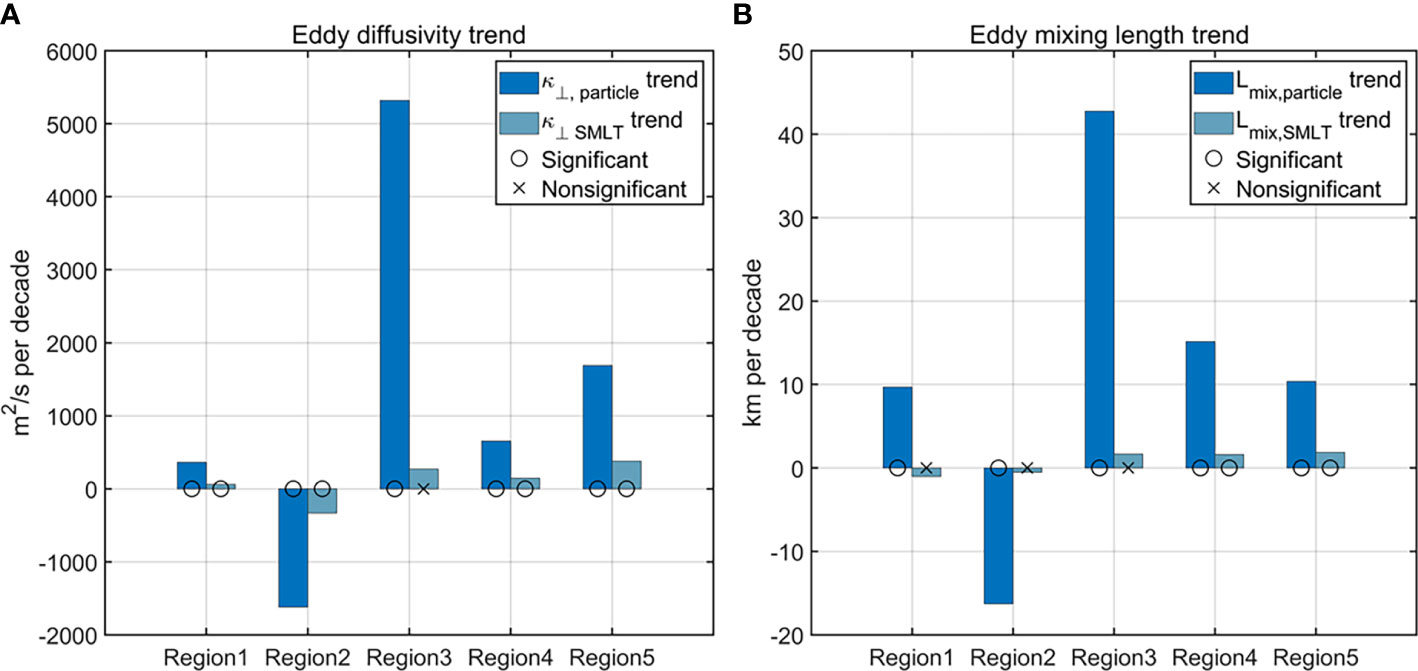
Figure 8 Trends in (A) eddy diffusivity and (B) eddy mixing length from the particle-based and SMLT-based methods in the representative regions shown in Figure 3. Statistically insignificant trends at the 95% confidence level are marked by “ $\times$“, and significant trends are marked by “$\circ$“.

The decomposition of the $L_{mix,SMLT}$ trend, based on Equation (12), reveals that among the three factors ($L_{eddy}$, $u_{rms}$, and $c_w-\left|{\text{U}}_g\right|$), $u_{rms}$ plays a dominant role in determining the trend in $L_{mix,SMLT}$. On the other hand, the trend in $c_w-\left|U_g\right|$ plays a negative role in the trend of eddy mixing length. As shown in Figure 9, in all the five regions, the relative trend in term $S1$ is larger than those in $S_2$ and $L_{eddy}$. Note that $S1$ represents the contribution of $u_{rms}$ to the $L_{mix,SMLT}$ trend. Therefore, besides acting as a direct and important governor of the eddy diffusivity trend (Figure 4B), $u_{rms}$ also play an indirect role in modulating eddy diffusivity trend through influencing the eddy mixing length (Figure 9). Although the relative trends of $L_{eddy}$ and $S1$ have comparable magnitudes in Region 3, the relative trend of $L_{eddy}$ is much smaller than that of $S1$ in the other regions, indicating a relative small role of $L_{eddy}$ in influencing the $L_{mix,SMLT}$ trend. In all the regions except Region 3, the sign of the relative trend in $S2$ is opposite to that of $L_{mix,SMLT}$. Therefore, in these regions, $c_w-\left|{\text{U}}_g\right|$ plays a negative role in the trend of eddy mixing length. Considering that the SMLT-based and particle-based eddy mixing lengths have the same trend sign in Regions 4 and 5, the SMLT results in these two regions can, to a certain degree, indicate the underlying mechanism of the particle-based eddy mixing length trend. However, in the other three regions (Regions 1-3), the sign of the trend in SMLT-based mixing length differs from that of particle-based mixing length. Therefore, SMLT cannot be used to explain mixing-length trends in Regions 1-3.

FIGURE 9

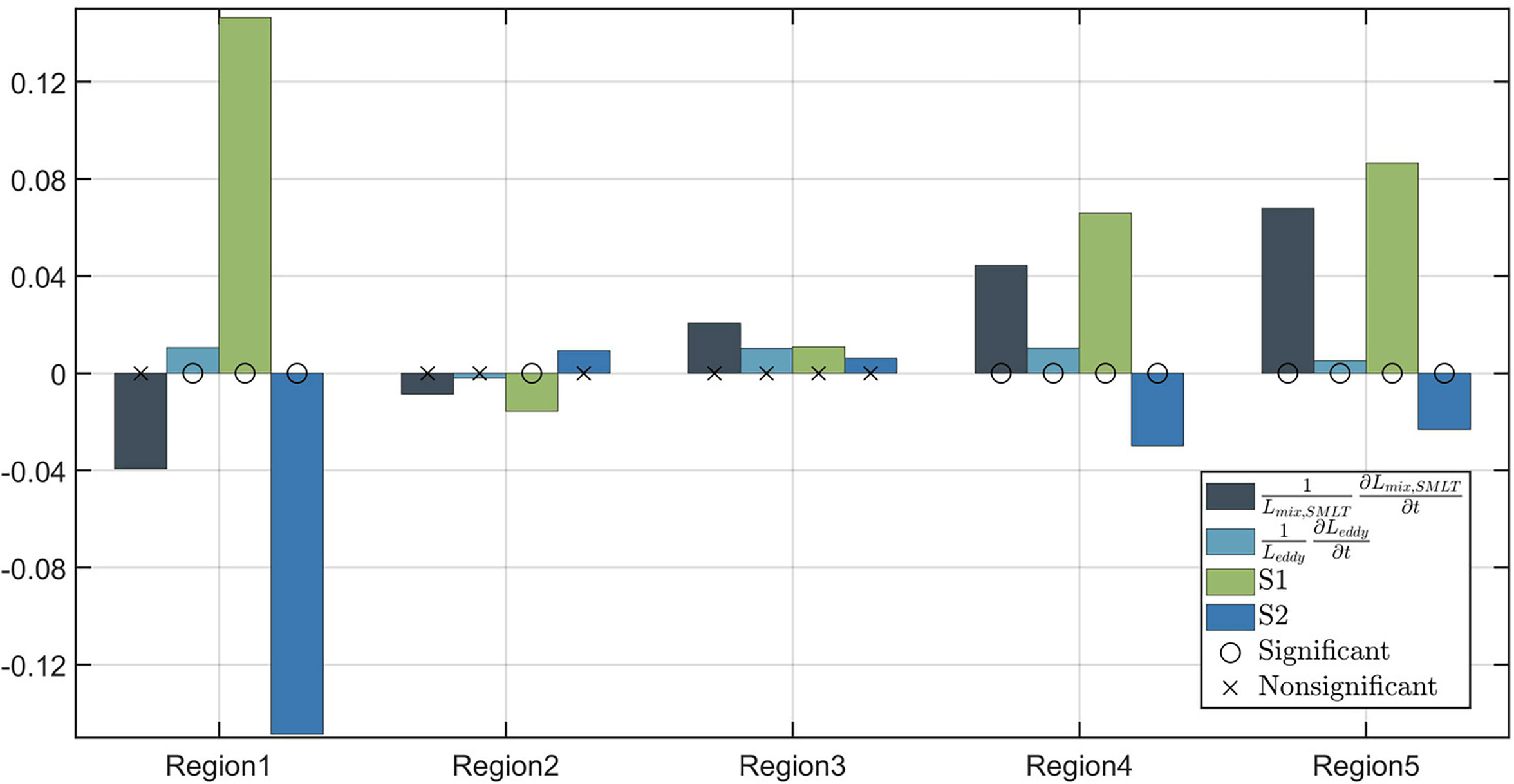
Figure 9 The relative trends of $L_{mix,SMLT}$, $L_{eddy}$, $S1$, and $S2$ from Equation (12) in the representative regions. The trends that are statistically insignificant at the 95% confidence level are marked by “ $\times$“, and those significant ones are marked by “$\circ$“.

Here we compare the trends in eddy properties with the mixing trends (Figure 10). In all the selected regions, the trend in eddy size ($L_{eddy}$) has the same sign as the trends in the particle-based eddy mixing length ($L_{mix,particle}$) and eddy diffusivity (${\kappa }_{\perp ,particle}$). This indicates that a positive response of the long-term variation of $L_{mix,particle}$ and ${\kappa }_{\perp ,particle}$ to the variability in $L_{eddy}$. However, though the trend in $c_w-\left|{\text{U}}_g\right|$ also has consistent sign with those in $L_{mix,particle}$ and ${\kappa }_{\perp ,particle}$ in all the regions except Region 3 (Figure 10B), $c_w-\left|{\text{U}}_g\right|$ and $L_{eddy}$ play opposite roles in shaping the mixing trends [see Equation (12)]. Similarly, in all these regions, the trend signs of $u_{rms}$ are consistent with those of $L_{mix,particle}$ and ${\kappa }_{\perp ,particle}$ (Figure 9C). This indicates that $u_{rms}$ plays a positive role in the mixing trends, consistent with the mixing length theory [Equation(5)] and SMLT [Equation (10)].

FIGURE 10

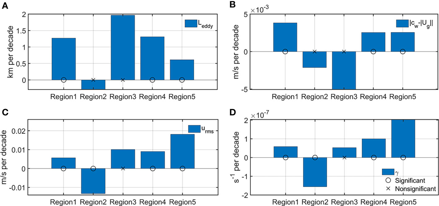
Figure 10 Trends of eddy/mean flow parameters from SMLT in the representative regions shown in Figure 3. (A) $L_{eddy}$. (B) $\left|c_w-\right|{\text{U}}_g\left|\right|$. (C) $u_{rms}$. (D) $\gamma$. The trends that are statistically insignificant at the 95% confidence level are marked by “ $\times$“, and those significant ones are marked by “$\circ$“.

5.2 Trends in eddy/mean flow properties

We further depict the regional trends in the eddy flow properties that are linked with the SMLT-based eddy diffusivity: Eddy size ($L_{eddy}$), the propagating speed of eddies relative to the mean flow ($c_w-\left|{\text{U}}_g\right|$), eddy velocity magnitude ($u_{rms}$) and the inverse of the eddy decorrelation time scale ($\gamma$) (Figure 10). In Regions 1, 4 and 5, eddy gets larger, more energetic, and propagate faster relative to the mean flow during the period 1997-2017. However, in these three regions, the inverse of the eddy decorrelation time scale has an increasing trend, indicating a faster decay of eddies during this period. In contrast, in Region 2, eddies get less energetic and decay more slowly during this time period. Yet, the trends in eddysize and eddy propagating speed relative to the mean flow are statistically nonsignificant. In Region 3, however, there are no statistically significant trends in all the four eddy properties.

Note that our trends in eddy properties can be interpreted based on previous studies about eddy dynamics. Firstly, we found that faster (slower) propagating speed of eddies relative to the mean flow generally corresponds to smaller (larger) eddy decorrelation time scale, i.e., faster (slower) eddy decay (Figures 10B, D). This phenomenon is consistent with the observation finding by Liu et al. (2022). Through both observations and idealized experiments, they demonstrate that a stronger Rossby wave phase speed leads to fast radiation of eddy energy and thus shorter eddy lifespan. Secondly, faster (slower) propagating speed of eddies relative to the mean flow often corresponds larger (smaller) eddy size. Specifically, in Regions 1, 4 and 5, the trends in $c_w-\left|{\text{U}}_g\right|$ and $L_{eddy}$ are both statistically significant and they have the same signs. This is to a certain extent related to the following previous findings. Klocker and Marshall (2014) found that eddy phase speed is generally consistent with the phase speed of linear, long Rossby waves that are Doppler shifted with the barotropic mean flow. Specifically, they show that the eddy propagation speed relative to the barotropic mean flow is $\beta L_D^2$, where $L_D$ is the Rossby deformation radius. In general, $L_D$ can be an approximate substitute for $L_{eddy}$ (Tulloch et al., 2011; Klocker and Abernathey, 2014). Therefore, it is unsurprising that $c_w-\left|{\text{U}}_g\right|$ has consistent trend sign with $L_{eddy}$. One caveat of this interpretation is that $U_g$ here is the surface geostrophic mean flow magnitude, not the barotropic mean flow considered in Klocker and Marshall (2014).

6 Interpreting trends in eddy velocity magnitude

Mixing length theory indicates that eddy diffusivity is proportional to the product of eddy mixing length and eddy velocity magnitude $u_{rms}$ [Equation (5)]. Here we interpret the trends in $u_{rms}$ using the geostrophic EKE budget, which is a key step towards unravelling the mechanism of the mixing-length trend.

6.1 Geostrophic EKE budget

To investigate the mechanism of the trend in $u_{rms}$ (surface geostrophic eddy velocity magnitude), we chose to derive and diagnose the budget equation of the surface geostrophic EKE (for details, see Supplementary Material). The formulation of the framework is inspired by the eddy/mean energy diagnostic framework from Chen et al. (2014a). But different from Chen et al. (2014a), our derivation here separately considers the geostrophic and ageostrophic EKE,

$\begin{array}{ll}\frac{\partial \overline{K_{E,g}}}{\partial t}=AD{V}_g+M_{K_{E,g}}+P{W}_H+R.& (13)\end{array}$

Here $K_{E,g}$ refers to the geostrophic EKE

$\begin{array}{ll}{K}_{E,g}=\frac{1}{2}{\rho }_0\overline{(u_g^{\text{'}2}+v_g^{\text{'}2})},& (14)\end{array}$

where ${\rho }_0$ is the sea surface density and takes a constant of 1027.5 kg m^-3. The overbar refers to the annual-mean over each year and ${·}^{\prime }$ denotes the deviation from the mean.

The mathematical formulas and the physical meanings of the terms on the right-hand side of Equation (13) are provided in Table 1. Equation (13) indicates that the trend in the geostrophic EKE may be induced by geostrophic advection ($AD{V}_g$), the geostrophic contribution to the eddy-mean kinetic energy exchange rate ($M_{K_{E,g}}$), the pressure work due to the horizontal ageostrophic flow ($P{W}_H$) and the residual term ($R$). As shown in Table 1, the residual term, $R$, includes four components: energy advection related to ageostrophic flow ($AD{V}_r$), the contribution of ageostrophic flow to the eddy-mean kinetic energy exchange rate ($M_{K_{E,r}}$), the change of EKE due to vertical and horizontal friction ($X_{K_E}$), and the temporal change rate of $K_{E,r}$. Among these components, $AD{V}_r$, $M_{K_{E,r}}$ and $\frac{\partial \overline{K_{E,r}}}{\partial t}$ can be diagnosed from

TABLE 1

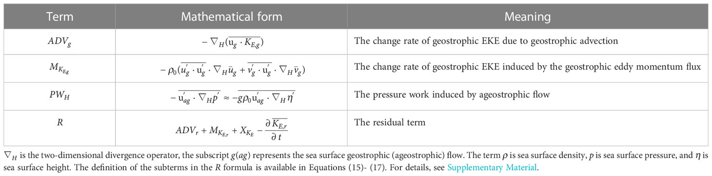
Table 1 The mathematical formulas and physical meanings of the terms on the right hand side of Equation (13).

$\begin{array}{ll}AD{V}_r=\underset{AD{V}_o}{\underbrace{-{\nabla }_H(\overline{{\text{u}}_o·0.5{\rho }_0(u_o^{\text{'}2}+v_o^{\text{'}2})})}}-AD{V}_g,& (15)\end{array}$

$\begin{array}{ll}{M}_{K_{E,r}}=\underset{M_{K_{E,o}}}{\underbrace{-{\rho }_0(\overline{u_o^{\text{'}}·{\text{u}}_o^{\text{'}}}·{\nabla }_H{\overline{u}}_o+\overline{v_o^{\text{'}}·{\text{u}}_o^{\text{'}}}·{\nabla }_H{\overline{v}}_o)}}-M_{K_{E,g}},& (16)\end{array}$

$\begin{array}{ll}\frac{\partial \overline{K_{E,r}}}{\partial t}=\frac{\partial \overline{\left[\frac{1}{2}{\rho }_0\left(u_o^{\text{'}2}+v_o^{\text{'}2}\right)\right]}}{\partial t}-\frac{\partial \overline{K_{E,g}}}{\partial t}.& (17)\end{array}$

Here $u_o$ and $v_o$ refer to the total surface velocity in the zonal and meridional direction. The ageostrophic velocity is defined as the difference between the total surface velocity and the geostrophic velocity,

$\begin{array}{ll}{\mathbf{\text{u}}}_{ag}={\mathbf{\text{u}}}_o-{\mathbf{\text{u}}}_g.& (18)\end{array}$

The full velocity ${\text{u}}_o$ is available from the OSCAR dataset, and the geostrophic velocity ${\text{u}}_g$ and sea surface height $\eta$ are available from the AVISO dataset. Therefore, one can directly diagnose all the terms in Equation (13) except for the $R$ term. Then we can approximately infer the value of $R$ by closing the $K_{E,g}$ budget. Concerning the terms in the $R$ equation (Table 1), using OSCAR and AVISO data, we can directly diagnose $AD{V}_r$, $M_{K_{E,r}}$ and $\frac{\partial K_{E,r}}{\partial t}$. The $X$ term is not explicitly diagnosed due to the absence of observed horizontal/vertical friction information.

6.2 Geostrophic EKE budget trends

To explore the origin of the trends in the surface geostrophic EKE and thus $u_{rms}$, we diagnosed the geostrophic EKE budget for each year [Equation (13)]. Then we estimated the trends in each term during the period 1994-2017. As shown in Figure 11, in all selected regions, the trends of $AD{V}_g$ and $M_{K_{E,g}}$ are generally small, with magnitudes on the order of 10^-7~10^-8 J m^-3. In contrast, the trends in $P{W}_H$ and $R$ are on the order of 10^-5~10^-6 J m^-3, much larger than those in $AD{V}_g$ and $M_{K_{E,g}}$. Therefore, in these five representative regions, the trends in the surface geostrophic EKE are mainly induced by the pressure work due to the horizontal ageostrophic flow ($P{W}_H$) and the residual term ($R$).

FIGURE 11

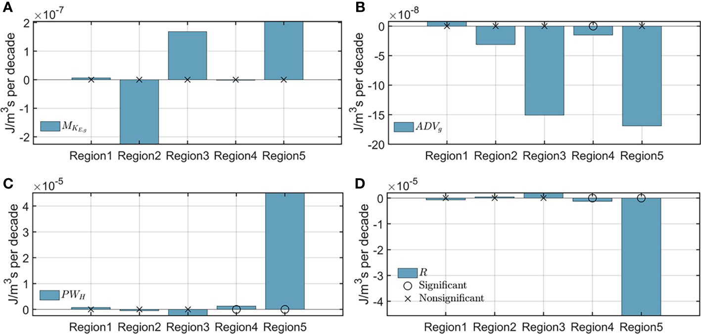
Figure 11 The trend in each term from the geostrophic EKE budget [Equation (13)] in the representative regions. (A) $M_{K_{E,g}}$. (B) $AD{V}_g$. (C) $P{W}_H$. (D) $R$. Statistically insignificant trends at the 95% confidence level are marked by “ $\times$“, and significant trends are marked by “$\circ$“.

The trends in $P{W}_H$ are statistically significant at the 95% confidence level in Regions 4 and 5. In these two regions, the trends in $P{W}_H$ and $u_{rms}$ have consistent signs (Figures 10C, 11C). Therefore, in Regions 4 and 5, the trend in pressure work ($P{W}_H$) contributes to the trend in $u_{rms}$. Using the classical linear Ekman theory, we express $P{W}_H$ as a function of wind stress and geostrophic flow (see Supplementary Material 3 for details). A series of studies have shown that both wind speed and ocean currents are accelerating (Hu et al., 2020; Peng et al., 2022). Much evidence have demonstrated that the increasing trend of EKE in the Southern Ocean is associated with enhanced wind stress (Sallee et al., 2011; Hogg et al., 2015; Mudelsee, 2019; Cai et al., 2022). In our study, Regions 4 and 5 are within the Southern Ocean. Similarly, in the western boundary current regions, Beal and Elipot (2016) found that the enhanced wind power leads to the strengthening of EKE. Therefore, the acceleration of the wind and the geostrophic flow may jointly induce the trend in the pressure work ($P{W}_H$).

Using the OSCAR and AVISO datasets, we also diagnosed the energy terms in the $R$ equation (Table 1). We estimated the $AD{V}_r$ and $M_{K_{E,r}}$ terms [Equations (15) and (16)], which are the part of the advection and eddy-mean energy exchange rate terms related to ageostrophic flow. The term $X_{K_E}$ is inferred from the other terms in the $R$ equation (Table 1). In all the five regions, the trends in both $AD{V}_r$ and $M_{K_{E,r}}$ are on the order of 10^-7~10^-8 J m^-3, whereas the trend in $X_{K_E}$ is on the order of 10^-5~10^-6 J m^-3 (not shown). Therefore, the leading contributor to the trend in $R$ is $X_{K_E}$, which denotes the EKE change rate due to horizontal/vertical friction. One caveat, however, is that uncertainties exist in our estimation of $X_{K_E}$. Example sources of uncertainty are provided next. One, our derivation of the geostrophic EKE budget [Equation (13)] ignores the contribution of vertical velocity to advection and eddy-mean energy exchange terms. Furthermore, the gridded AVISO dataset averages out the high-frequency ocean motions (e.g., internal tides). These issues would lead to uncertainties in our inference of $R$. In addition, the ageostrophic flow from OSCAR is to a large extent the Ekman flow and thus it does not include the submesoscale component of the ageostrophic flow. In consequence, our estimation of $AD{V}_r$, $M_{K_{E,r}}$ and $\frac{\partial K_{E,r}}{\partial t}$ excludes the contribution of oceanic submesoscales, which may be non-negligible. The estimates of $R$ and $X_{K_E}$ terms could be improved as the resolution of satellite observation increases. Further investigation along this line is left for future work.

7 Conclusion

Using the AVISO observations during 1994-2017, this study estimated the trend in particle-based eddy diffusivity (${\kappa }_{\perp ,particle}$) at the global surface ocean. The spatial structure of this eddy mixing trend has large regional variability. In 54% of the global ocean, ${\kappa }_{\perp ,particle}$ shows an increasing trend. The globally integrated ${\kappa }_{\perp ,particle}$ shows a significant increasing trend, with an increase of 284.1 ${\text{m}}^2{\text{s}}^{-1}$ per decade, accounting for 3.7% of the climate mean value. Using a trend decomposition method (Guo et al., 2022) and the mixing length theory, we found that the relative trend of ${\kappa }_{\perp ,particle}$ is equal to the sum of the relative trend in eddy mixing length ($L_{mix}$) and that of eddy velocity magnitude ($u_{rms}$). In 73% of the global ocean, $L_{mix}$ contributes more to the relative trend in eddy diffusivity than $u_{rms}$. Therefore, in these regions, the main direct source of the ${\kappa }_{\perp ,particle}$ trend is the trend in $L_{mix}$, not that in $u_{rms}$. Yet, the contribution of $u_{rms}$ is also noticeable.

Since $L_{mix}$ and $u_{rms}$ jointly determine eddy diffusivity, we explore the mechanism of eddy mixing trends by interpreting the trends in $L_{mix}$ and $u_{rms}$, respectively. We chose to discuss the mechanism of the $L_{mix}$ trend using SMLT and its trend decomposition. SMLT well captures the trend sign of the particle-based eddy mixing lengths in two of the five regions, i.e., Regions 4 and 5. The trends in eddy/mean flow parameters related to SMLT (e.g., eddy size, $u_{rms}$, the propagating speed of eddies relative to the mean flow, and the inverse of the eddy decorrelation time scale) jointly determine the trend in the SMLT-based mixing length. Among these parameters, $u_{rms}$ plays a dominant role in determining the SMLT-based $L_{mix}$ trend. We also found that $u_{rms}$ dose not only directly modulate the trend in eddy mixing, but also indirectly affect the eddy diffusivity trend through its link with the $L_{mix}$.

We then discuss the trend in $u_{rms}$, which also help unravel the origin of the eddy mixing trend. By diagnosing a novel surface geostrophic EKE budget, we found that pressure work due to the horizontal ageostrophic flow plays a dominant role in the trend in $u_{rms}$. Then using the classical linear Ekman theory, we developed a formula linking pressure work with wind stress and geostrophic flow. This formula and evidence in literature (e.g., Sallee et al., 2011; Hogg et al., 2015; Mudelsee, 2019; Hu et al., 2020; Cai et al., 2022; Peng et al., 2022) suggests that the acceleration of wind and geostrophic flow might jointly induce the trend in pressure work.

There are potential avenues to further improve this work. One, this study focuses on the surface ocean. The mixing trend at mid-depths and in the deep ocean remains unclear. Also it would be worthwhile evaluating whether this observed mixing trend is well captured in the widely-used numerical products (Ma et al., 2010; Yang et al., 2018; Xu et al., 2021). Two, the mechanisms of the trends in relevant eddy properties (e.g., eddy size and eddy phase speed) need to be further explored. This effort would help design eddy parameterization schemes taking into account mixing trend.

One caveat of this work is that uncertainties remain in our mixing trend estimation. The data duration we use is only 24 years and a longer time series may lead to a more robust estimation of the long-term trend (Beech et al., 2022). Therefore, though expensive, continuous observations of the oceanic currents and other relevant tracer variables (e.g., temperature) would be valuable for more accurate trend estimation.

Despite the uncertainties in our trend estimation, our results clearly indicate that there is regional long-term adjustment of mesoscale eddies throughout the ocean. As the ocean’s response to climate change is slow, ocean changes, including the changes in eddy mixing, will continue building up. The eddy adjustment may significantly affect the distribution of key tracers in the ocean (e.g., heat, salt, and nutrient) and thus change the water mass distribution and air-sea interaction. This in turn would lead to the variability of the ocean circulation, climate system and marine ecosystem. Therefore, it could be useful to fully consider the long-term trends in eddy mixing when implementing eddy parameterization schemes in non-eddy-resolving climate models.

Data availability statement

The original contributions presented in the study are included in the article/Supplementary Material. Further inquiries can be directed to the corresponding author.

Author contributions

RC and GZ conceived this project. RC conducted the particle-tracking experiments and formulated the diagnosis frameworks. GZ analyzed the data and wrote the initial draft. RC, LL, HW and SS reviewed and revised the manuscript. All authors interpreted the results and approved the submitted version.

Funding

This work was supported by the National Natural Science Foundation of China through 42076007. LL is partially supported by the seed grant from the Institute of Computational and Data Sciences at the Pennsylvania State University.

Acknowledgments

We thank Wenting Guan for her technical assistance about eddy diffusivity estimates, and Qianqian Geng for proofreading and editing the manuscript. h T. Gille and Julie L. McClean from Scripps Institution of Oceanography at the University of California, San Diego for introducing us to the topic of Lagrangian eddy diffusivities.

Conflict of interest

The authors declare that the research was conducted in the absence of any commercial or financial relationships that could be construed as a potential conflict of interest.

Publisher’s note

All claims expressed in this article are solely those of the authors and do not necessarily represent those of their affiliated organizations, or those of the publisher, the editors and the reviewers. Any product that may be evaluated in this article, or claim that may be made by its manufacturer, is not guaranteed or endorsed by the publisher.

Supplementary material

The Supplementary Material for this article can be found online at: https://www.frontiersin.org/articles/10.3389/fmars.2023.1157049/full#supplementary-material

References

Abernathey R. P., Marshall J. (2013). Global surface eddy diffusivities derived from satellite altimetry. J. Geophys. Res.: Oceans 118, 901–916. doi: 10.1002/jgrc.20066

CrossRef Full Text | Google Scholar

Abernathey R., Marshall J., Ferreira D. (2011). The dependence of southern ocean meridional overturning on wind stress. J. Phys. Oceanogr. 41, 2261–2278. doi: 10.1175/JPO-D-11-023.1

CrossRef Full Text | Google Scholar

Bates M., Tulloch R., Marshall J., Ferrari R. (2014). Rationalizing the spatial distribution of mesoscale eddy diffusivity in terms of mixing length theory. J. Phys. Oceanogr. 44, 1523–1540. doi: 10.1175/JPO-D-13-0130.1

CrossRef Full Text | Google Scholar

Beal L. M., Elipot S. (2016). Broadening not strengthening of the agulhas current since the early 1990s. Nature 540, 570–573. doi: 10.1038/nature19853

PubMed Abstract | CrossRef Full Text | Google Scholar

Beech N., Rackow T., Semmler T., Danilov S., Wang Q., Jung T. (2022). Long-term evolution of ocean eddy activity in a warming world. Nat. Climate Change 12, 910–917. doi: 10.1038/s41558-022-01478-3

CrossRef Full Text | Google Scholar

Bolton T., Abernathey R., Zanna L. (2019). Regional and temporal variability of lateral mixing in the north Atlantic. J. Phys. Oceanogr. 49, 2601–2614. doi: 10.1175/JPO-D-19-0042.1

CrossRef Full Text | Google Scholar

Bonjean F., Lagerloef G. S. (2002). Diagnostic model and analysis of the surface currents in the tropical pacific ocean. J. Phys. Oceanogr. 32, 2938–2954. doi: 10.1175/1520-0485(2002)032<2938:DMAAOT>2.0.CO;2

CrossRef Full Text | Google Scholar

Busecke J. J., Abernathey R. P. (2019). Ocean mesoscale mixing linked to climate variability. Sci. Adv. 5, eaav5014. doi: 10.1126/sciadv.aav5014

PubMed Abstract | CrossRef Full Text | Google Scholar

Busecke J., Abernathey R. P., Gordon A. L. (2017). Lateral eddy mixing in the subtropical salinity maxima of the global ocean. J. Phys. Oceanogr. 47, 737–754. doi: 10.1175/JPO-D-16-0215.1

CrossRef Full Text | Google Scholar

Cai Y., Chen D., Mazloff M. R., Lian T., Liu X. (2022). Topographic modulation of the wind stress impact on eddy activity in the southern ocean. Geophys. Res. Lett. 49, e2022GL097859. doi: 10.1029/2022GL097859

CrossRef Full Text | Google Scholar

Chen R., Flierl G. R., Wunsch C. (2014a). A description of local and nonlocal eddy–mean flow interaction in a global eddy-permitting state estimate. J. Phys. Oceanogr. 44, 2336–2352. doi: 10.1175/JPO-D-14-0009.1

CrossRef Full Text | Google Scholar

Chen R., Gille S. T., McClean J. L. (2017). Isopycnal eddy mixing across the kuroshio extension: stable versus unstable states in an eddying model. J. Geophys. Res.: Oceans 122, 4329–4345. doi: 10.1002/2016JC012164

CrossRef Full Text | Google Scholar

Chen R., Gille S., McClean J., Flierl G., Griesel A. (2015). A multiwavenumber theory for eddy diffusivities and its application to the southeast pacific (DIMES) region. J. Phys. Oceanogr. 45, 1877–1896. doi: 10.1175/JPO-D-14-0229.1

CrossRef Full Text | Google Scholar

Chen G., Li Y., Xie Q., Wang D. (2018). Origins of eddy kinetic energy in the bay of Bengal. J. Geophys. Res.: Oceans 123, 2097–2115. doi: 10.1002/2017JC013455

CrossRef Full Text | Google Scholar

Chen R., Mcclean J. L., Gille S. T., Griesel A. (2014b). Isopycnal eddy diffusivities and critical layers in the kuroshio extension from an eddying ocean model. J. Phys. Oceanogr. 44, 2191–2211. doi: 10.1175/JPO-D-13-0258.1

CrossRef Full Text | Google Scholar

Chen R., Waterman S. (2017). Mixing nonlocality and mixing anisotropy in an idealized western boundary current jet. J. Phys. Oceanogr. 47, 3015–3036. doi: 10.1175/JPO-D-17-0011.1

CrossRef Full Text | Google Scholar

Chernick M. R. (2011). Bootstrap methods: a guide for practitioners and researchers (John Wiley & Sons).

Google Scholar

Church J. A., White N. J., Konikow L. F., Domingues C. M., Cogley J. G., Rignot E., et al. (2011). Revisiting the earth’s sea-level and energy budgets from 1961 to 2008. Geophys. Res. Lett. 38 (18), L18601. doi: 10.1029/2011GL048794

CrossRef Full Text | Google Scholar

Danabasoglu G., Marshall J. (2007). Effects of vertical variations of thickness diffusivity in an ocean general circulation model. Ocean Model. 18, 122–141. doi: 10.1016/j.ocemod.2007.03.006

CrossRef Full Text | Google Scholar

Davis R. E. (1987). Modeling eddy transport of passive tracers. J. Mar. Res. 45, 635–666. doi: 10.1357/002224087788326803

CrossRef Full Text | Google Scholar

Davis R. E. (1991). Observing the general circulation with floats. Deep Sea Res. Part A. Oceanogr. Res. Pap. 38, 531–571. doi: 10.1016/S0198-0149(12)80023-9

CrossRef Full Text | Google Scholar

Dohan K. (2017). Ocean surface currents from satellite data. J. Geophys. Res.: Oceans 122, 2647–2651. doi: 10.1002/2017JC012961

CrossRef Full Text | Google Scholar

Du Y., Zhang Y., Feng M., Wang T., Zhang N., Wijffels S. (2015). Decadal trends of the upper ocean salinity in the tropical indo-pacific since mid-1990s. Sci. Rep. 5, 1–9. doi: 10.1038/srep16050

CrossRef Full Text | Google Scholar

Ferrari R., Nikurashin M. (2010). Suppression of eddy diffusivity across jets in the southern ocean. J. Phys. Oceanogr. 40, 1501–1519. doi: 10.1175/2010JPO4278.1

CrossRef Full Text | Google Scholar

Ferrari R., Wunsch C. (2009). Ocean circulation kinetic energy: reservoirs, sources, and sinks. Annu. Rev. Fluid Mech. 41, 253–282. doi: 10.1146/annurev.fluid.40.111406.102139

CrossRef Full Text | Google Scholar

Fox-Kemper B., Adcroft A., Böning C. W., Chassignet E. P., Curchitser E., Danabasoglu G., et al. (2019). Challenges and prospects in ocean circulation models. Front. Mar. Sci. 6, 65. doi: 10.3389/fmars.2019.00065

CrossRef Full Text | Google Scholar

Gent P. R., Mcwilliams J. C. (1990). Isopycnal mixing in ocean circulation models. J. Phys. Oceanogr. 20, 150–155. doi: 10.1175/1520-0485(1990)020<0150:IMIOCM>2.0.CO;2

CrossRef Full Text | Google Scholar

Gnanadesikan A., Pradal M., Abernathey R. (2015). Isopycnal mixing by mesoscale eddies significantly impacts oceanic anthropogenic carbon uptake. Geophys. Res. Lett. 42, 4249–4255. doi: 10.1002/2015GL064100

CrossRef Full Text | Google Scholar

Gnanadesikan A., Russell A., Pradal M. A., Abernathey R. (2017). Impact of lateral mixing in the ocean on El nino in a suite of fully coupled climate models. J. Adv. Model. Earth Syst. 9, 2493–2513. doi: 10.1002/2017MS000917

CrossRef Full Text | Google Scholar

Gocic M., Trajkovic S. (2013). Analysis of changes in meteorological variables using Mann-Kendall and sen’s slope estimator statistical tests in Serbia. Global Planet. Change 100, 172–182. doi: 10.1016/j.gloplacha.2012.10.014

CrossRef Full Text | Google Scholar

Green J. S. A. (1970). Transfer properties of the large-scale eddies and the general circulation of the atmosphere. Q. J. R. Meteorol. Soc. 96, 157–185. doi: 10.1002/qj.49709640802

CrossRef Full Text | Google Scholar

Griesel A., Gille S. T., Sprintall J., McClean J. L., Lacasce J. H., Maltrud M. E. (2010). Isopycnal diffusivities in the Antarctic circumpolar current inferred from Lagrangian floats in an eddying model. J. Geophys. Res.: Oceans 115, C06006. doi: 10.1029/2009JC005821

CrossRef Full Text | Google Scholar

Griesel A., Mcclean J. L., Gille S. T., Sprintall J., Eden C. (2014). Eulerian and Lagrangian isopycnal eddy diffusivities in the southern ocean of an eddying model. J. Phys. Oceanogr. 44, 644–661. doi: 10.1175/JPO-D-13-039.1

CrossRef Full Text | Google Scholar

Griffies S. M. (1998). The gent–mcwilliams skew flux. J. Phys. Oceanogr. 28, 831–841. doi: 10.1175/1520-0485(1998)028<0831:TGMSF>2.0.CO;2

CrossRef Full Text | Google Scholar

Groeskamp S., LaCasce J. H., McDougall T. J., Rogé M. (2020). Full-depth global estimates of ocean mesoscale eddy mixing from observations and theory. Geophys. Res. Lett. 47, e2020GL089425. doi: 10.1029/2020GL089425

CrossRef Full Text | Google Scholar

Guan W., Chen R., Zhang H., Yang Y., Wei H. (2022). Seasonal surface eddy mixing in the kuroshio extension: estimation and machine learning prediction. J. Geophys. Res.: Oceans 127, e2021JC017967. doi: 10.1029/2021JC017967

CrossRef Full Text | Google Scholar

Guo Y., Bachman S., Bryan F., Bishop S. (2022). Increasing trends in oceanic surface poleward eddy heat flux observed over the past three decades. Geophys. Res. Lett. 49, e2022GL099362. doi: 10.1029/2022GL099362

CrossRef Full Text | Google Scholar

Hamed K. H., Rao A. R. (1998). A modified Mann-Kendall trend test for autocorrelated data. J. hydrol. 204, 182–196. doi: 10.1016/S0022-1694(97)00125-X

CrossRef Full Text | Google Scholar

Hogg A. M., Meredith M. P., Chambers D. P., Abrahamsen E. P., Hughes C. W., Morrison A. K. (2015). Recent trends in the southern ocean eddy field. J. Geophys. Res.: Oceans 120, 257–267. doi: 10.1002/2014JC010470

CrossRef Full Text | Google Scholar

Hu S., Sprintall J., Guan C., McPhaden M. J., Wang F., Hu D., et al. (2020). Deep-reaching acceleration of global mean ocean circulation over the past two decades. Sci. Adv. 6, eaax7727. doi: 10.1126/sciadv.aax7727

PubMed Abstract | CrossRef Full Text | Google Scholar

Ivanova D. P., McClean J. L., Sprintall J., Chen R. (2021). The oceanic barrier layer in the eastern Indian ocean as a predictor for rainfall over Indonesia and Australia. Geophys. Res. Lett. 48, e2021GL094519. doi: 10.1029/2021GL094519

CrossRef Full Text | Google Scholar

Jansen M. F., Adcroft A. J., Hallberg R., Held I. M. (2015). Parameterization of eddy fluxes based on a mesoscale energy budget. Ocean Model. 92, 28–41. doi: 10.1016/j.ocemod.2015.05.007

CrossRef Full Text | Google Scholar

Johnson G. C., Lyman J. M. (2020). Warming trends increasingly dominate global ocean. Nat. Climate Change 10, 757–761. doi: 10.1038/s41558-020-0822-0

CrossRef Full Text | Google Scholar

Kendall M. G. (1948). Rank correlation methods.

Google Scholar

Klocker A., Abernathey R. (2014). Global patterns of mesoscale eddy properties and diffusivities. J. Phys. Oceanogr. 44, 1030–1046. doi: 10.1175/JPO-D-13-0159.1

CrossRef Full Text | Google Scholar

Klocker A., Ferrari R., Lacasce J. H. (2012b). Estimating suppression of eddy mixing by mean flows. J. Phys. Oceanogr. 42, 1566–1576. doi: 10.1175/JPO-D-11-0205.1

CrossRef Full Text | Google Scholar

Klocker A., Ferrari R., Lacasce J. H., Merrifield S. T. (2012). Reconciling float-based and tracer-based estimates of lateral diffusivities. J. Mar. Res. 70, 569–602. doi: 10.1357/002224012805262743

CrossRef Full Text | Google Scholar

Klocker A., Marshall D. P. (2014). Advection of baroclinic eddies by depth mean flow. Geophys. Res. Lett. 41, 3517–3521. doi: 10.1002/2014GL060001

CrossRef Full Text | Google Scholar

Koszalka I. M., LaCasce J. H. (2010). Lagrangian Analysis by clustering. Ocean Dyn. 60, 957–972. doi: 10.1007/s10236-010-0306-2

CrossRef Full Text | Google Scholar

LaCasce J., Bower A. (2000). Relative dispersion in the subsurface north Atlantic. J. Mar. Res. 58, 863–894. doi: 10.1357/002224000763485737

CrossRef Full Text | Google Scholar

Lagerloef G. S., Mitchum G. T., Lukas R. B., Niiler P. P. (1999). Tropical pacific near-surface currents estimated from altimeter, wind, and drifter data. J. Geophys. Res.: Oceans 104, 23313–23326. doi: 10.1029/1999JC900197

CrossRef Full Text | Google Scholar

Landschützer P., Gruber N., Bakker D. C. (2016). Decadal variations and trends of the global ocean carbon sink. Global Biogeochem. Cycles 30, 1396–1417. doi: 10.1002/2015GB005359

CrossRef Full Text | Google Scholar

Lee K., Nam S., Cho Y.-K., Jeong K.-Y., Byun D.-S. (2022). Determination of long-term, (1993–2019) sea level rise trends around the Korean peninsula using ocean tide-corrected, multi-mission satellite altimetry data. Front. Mar. Sci. 9, 810549. doi: 10.3389/fmars.2022.810549

CrossRef Full Text | Google Scholar

Liu R., Wang G., Chapman C., Chen C. (2022). The attenuation effect of jet filament on the eastward mesoscale eddy lifetime in the southern ocean. J. Phys. Oceanogr. 52, 805–822. doi: 10.1175/JPO-D-21-0030.1

CrossRef Full Text | Google Scholar

Lumpkin R., Elipot S. (2010). Surface drifter pair spreading in the north Atlantic. J. Geophys. Res.: Oceans, 115, C120117. doi: 10.1029/2010JC006338

CrossRef Full Text | Google Scholar

Ma C., Yang J., Wu D., Lin X. (2010). The kuroshio extension: a leading mechanism for the seasonal sea-level variability along the west coast of Japan. Ocean Dyn. 60, 667–672. doi: 10.1007/s10236-009-0239-9

CrossRef Full Text | Google Scholar

Mann H. B. (1945). Nonparametric tests against trend. Econ.: J. econ. Soc. 13, 245–259. doi: 10.2307/1907187

CrossRef Full Text | Google Scholar

Martínez-Moreno J., Hogg A. M., England M. H., Constantinou N. C., Kiss A. E., Morrison A. K. (2021). Global changes in oceanic mesoscale currents over the satellite altimetry record. Nat. Climate Change 11, 397–403. doi: 10.1038/s41558-021-01006-9

CrossRef Full Text | Google Scholar

Mudelsee M. (2019). Trend analysis of climate time series: a review of methods. Earth-science Rev. 190, 310–322. doi: 10.1016/j.earscirev.2018.12.005

CrossRef Full Text | Google Scholar

Nan F., Yu F., Xue H., Wang R., Si G. (2015). Ocean salinity changes in the northwest pacific subtropical gyre: the quasi-decadal oscillation and the freshening trend. J. Geophys. Res.: Oceans 120, 2179–2192. doi: 10.1002/2014JC010536

CrossRef Full Text | Google Scholar

Naveira Garabato A. C., Ferrari R., Polzin K. L. (2011). Eddy stirring in the southern ocean. J. Geophys. Res.: Oceans 116, C09019. doi: 10.1029/2010JC006818

CrossRef Full Text | Google Scholar

Ohlson J. A., Kim S. (2015). Linear valuation without OLS: the theil-sen estimation approach. Rev. Accounting Stud. 20, 395–435. doi: 10.1007/s11142-014-9300-0

CrossRef Full Text | Google Scholar

Patara L., Böning C. W., Biastoch A. (2016). Variability and trends in southern ocean eddy activity in 1/12° ; ocean model simulations. Geophys. Res. Lett. 43, 4517–4523. doi: 10.1002/2016GL069026

CrossRef Full Text | Google Scholar

Peng Q., Xie S.-P., Wang D., Huang R. X., Chen G., Shu Y., et al. (2022). Surface warming–induced global acceleration of upper ocean currents. Sci. Adv. 8, eabj8394. doi: 10.1126/sciadv.abj8394

PubMed Abstract | CrossRef Full Text | Google Scholar

Piontkovski S. A., Al-Tarshi M. H., Al-Ismaili S. M., Al-Jardani S., Al-Alawi Y. (2019). Inter-annual variability of mesoscale eddy occurrence in the western Arabian Sea. Int. J. Oceans Oceanogr. 13, 1–23.

Google Scholar

Risaro D. B., Chidichimo M. P., Piola A. R. (2022). Interannual variability and trends of sea surface temperature around southern south America. Front. Mar. Sci. 9, 213. doi: 10.3389/fmars.2022.829144

CrossRef Full Text | Google Scholar

Roach C. J., Balwada D., Speer K. (2016). Horizontal mixing in the southern ocean from argo float trajectories. J. Geophys. Res.: Oceans 121, 5570–5586. doi: 10.1002/2015JC011440

CrossRef Full Text | Google Scholar

Roach C. J., Balwada D., Speer K. (2018). Global observations of horizontal mixing from argo float and surface drifter trajectories. J. Geophys. Res.: Oceans 123, 4560–4575. doi: 10.1029/2018JC013750

CrossRef Full Text | Google Scholar

Rypina I. I., Kamenkovich I., Berloff P., Pratt L. J. (2012). Eddy-induced particle dispersion in the near-surface north Atlantic. J. Phys. Oceanogr. 42, 2206–2228. doi: 10.1175/JPO-D-11-0191.1

CrossRef Full Text | Google Scholar

Sa’adi Z., Shahid S., Ismail T., Chung E.-S., Wang X.-J. (2019). Trends analysis of rainfall and rainfall extremes in Sarawak, Malaysia using modified Mann–Kendall test. Meteorol. Atmos. Phys. 131, 263–277. doi: 10.1007/s00703-017-0564-3

CrossRef Full Text | Google Scholar

Sallee J.-B., Speer K., Rintoul S. (2011). Mean-flow and topographic control on surface eddy-mixing in the southern ocean. J. Mar. Res. 69, 753–777. doi: 10.1357/002224011799849408

CrossRef Full Text | Google Scholar

Schulte J. A., Najjar R. G., Li M. (2016). The influence of climate modes on streamflow in the mid-Atlantic region of the united states. J. Hydrol.: Reg. Stud. 5, 80–99. doi: 10.1016/j.ejrh.2015.11.003

CrossRef Full Text | Google Scholar

Sen P. K. (1968). Estimates of the regression coefficient based on kendall’s tau. J. Am. Stat. Assoc. 63, 1379–1389. doi: 10.1080/01621459.1968.10480934

CrossRef Full Text | Google Scholar

Stammer D. (1998). On eddy characteristics, eddy transports, and mean flow properties. J. Phys. Oceanogr. 28, 727–739. doi: 10.1175/1520-0485(1998)028<0727:OECETA>2.0.CO;2

CrossRef Full Text | Google Scholar

Steinkamp K., Gruber N. (2015). Decadal trends of ocean and land carbon fluxes from a regional joint ocean-atmosphere inversion. Global Biogeochem. Cycles 29, 2108–2126. doi: 10.1002/2014GB004907

CrossRef Full Text | Google Scholar

Sun W., Yang J., Tan W., Liu Y., Zhao B., He Y., et al. (2021). Eddy diffusivity and coherent mesoscale eddy analysis in the southern ocean. Acta Oceanol. Sin. 40, 1–16. doi: 10.1007/s13131-021-1881-4

CrossRef Full Text | Google Scholar

Syst E., Attribution C. C., Global W., Level S., Group B., Cazenave A.. (2018). Global sea-level budget 1993 – Present. Earth Sys. Sci. Data 1 (3), 1551–1590. doi: 10.5194/essd-10-1551-2018

CrossRef Full Text | Google Scholar

Taylor G. I. (1915). I. eddy motion in the atmosphere. Philos. Trans. R. Soc. London. Ser. A Containing Pap. Math. Phys. Character 215, 1–26. doi: 10.1098/rsta.1915.0001

CrossRef Full Text | Google Scholar

Theil H. (1950). A rank-invariant method of linear and polynomial regression analysis, I, II, III, nederl. Akad. Wetensch. Proc. 53, 386–392, 521–525, 1397–1412. doi: 10.1007/978-94-011-2546-8_20

CrossRef Full Text | Google Scholar

Tulloch R., Marshall J., Hill C., Smith K. S. (2011). Scales, growth rates, and spectral fluxes of baroclinic instability in the ocean. J. Phys. Oceanogr. 41, 1057–1076. doi: 10.1175/2011JPO4404.1

CrossRef Full Text | Google Scholar

Wei H., Wang Y. (2021). Full-depth scalings for isopycnal eddy mixing across continental slopes under upwelling-favorable winds. J. Adv. Model. Earth Syst. 13, e2021MS002498. doi: 10.1029/2021MS002498

CrossRef Full Text | Google Scholar

Xu L., Ding Y., Xie S.-P. (2021). Buoyancy and wind driven changes in subantarctic mode water during 2004–2019. Geophys. Res. Lett. 48, e2021GL092511. doi: 10.1029/2021GL092511

CrossRef Full Text | Google Scholar

Yamaguchi R., Suga T. (2019). Trend and variability in global upper-ocean stratification since the 1960s. J. Geophys. Res.: Oceans 124, 8933–8948. doi: 10.1029/2019JC015439

CrossRef Full Text | Google Scholar

Yang H., Qiu B., Chang P., Wu L., Wang S., Chen Z., et al. (2018). Decadal variability of eddy characteristics and energetics in the kuroshio extension: unstable versus stable states. J. Geophys. Res.: Oceans 123, 6653–6669. doi: 10.1029/2018JC014081

CrossRef Full Text | Google Scholar

Yu X., Ponte A. L., Elipot S., Menemenlis D., Abernathey R. (2019). Surface kinetic energy distributions in the global oceans from a high-resolution numerical model and surface drifter observations. Geophys. Res. Lett. 46 (16), 9757–9766. doi: 10.1029/2019GL083074

CrossRef Full Text | Google Scholar

Yue S., Wang C. (2004). The Mann-Kendall test modified by effective sample size to detect trend in serially correlated hydrological series. Water Resour. Manage. 18, 201–218. doi: 10.1023/B:WARM.0000043140.61082.60

CrossRef Full Text | Google Scholar

Zhao B., Lin P., Hu A., Liu H., Ding M., Yu Z., et al. (2022). Uncertainty in Atlantic multidecadal oscillation derived from different observed datasets and their possible causes. Front. Mar. Sci. 9, 2148. doi: 10.3389/fmars.2022.1007646

CrossRef Full Text | Google Scholar

Zhurbas V., Oh S. I. (2004). Drifter-derived maps of lateral diffusivity in the pacific and Atlantic oceans in relation to surface circulation patterns. J. Geophys. Res. 109, C05015. doi: 10.1029/2003JC002241

CrossRef Full Text | Google Scholar