
94% of researchers rate our articles as excellent or good
Learn more about the work of our research integrity team to safeguard the quality of each article we publish.
Find out more
ORIGINAL RESEARCH article
Front. Mar. Sci., 08 August 2022
Sec. Aquatic Microbiology
Volume 9 - 2022 | https://doi.org/10.3389/fmars.2022.897140
 Leocadio Blanco-Bercial1*Rachel Parsons1Luis M. Bolaños2Rod Johnson1Stephen J. Giovannoni2Ruth Curry1
Protists represent the majority of the eukaryotic diversity in the oceans. They have different functions in the marine food web, playing essential roles in the biogeochemical cycles. While the available data is rich in horizontal and temporal coverage, little is known on their vertical structuring, particularly below the photic zone. The present study applies V4 18S rDNA metabarcoding to samples collected over three years in conjunction with the BATS time-series to assess marine protist communities in the epipelagic and mesopelagic zones (0-1000 m). The protist community showed a dynamic seasonality in the epipelagic, responding to hydrographic yearly cycles. Mixotrophic lineages dominated throughout the year. However, autotrophs bloomed during the rapid transition between the winter mixing and the stratified summer, and heterotrophs had their peak at the end of summer, when the base of the thermocline reaches its deepest depth. Below the photic zone, the community, dominated by Rhizaria, is depth-stratified and relatively constant throughout the year, although they followed local hydrographic and biological features such as the oxygen minimum zone. The results suggest a dynamic partitioning of the water column, where the niche vertical position for each community changes throughout the year in the epipelagic, likely depending on nutrient availability, the mixed layer depth, and other hydrographic features. At depth, the protist community closely tracked mesoscale events (eddies), where the communities followed the hydrographic uplift, raising the deeper communities for hundreds of meters, and compressing the communities above.
Marine protists encompass a large and heterogeneous community representing the majority of the eukaryotic diversity on the oceans (Worden et al., 2015). They include primary producers (autotrophs), heterotrophs (phagotrophs and parasitic), and a substantial collection of lineages exhibiting varying degrees of mixotrophic strategies (Mitra et al., 2016). These groups occupy distinct niches in the marine food web, playing essential roles in biogeochemical cycles (Mitra et al., 2014; Worden et al., 2015). They are responsible for ~50% of annual planktonic photosynthetic primary productivity (PP), of which they consume ~66%, plus an additional 10% of bacterial PP (Calbet and Landry, 2004; Steinberg and Landry, 2017). Recent applications of molecular tools such as metabarcoding (de Vargas et al., 2015; Choi et al., 2020), metagenomics and single cell genomics (Latorre et al., 2021), have significantly sharpened our understanding of protist diversity, distributions, and functionality, from basic trophic modes to complex metabolic pathways, and emphasized their importance in channeling marine productivity to upper trophic levels. The available observational data is rich in horizontal spatial and temporal coverage, yet lacks vertical resolution, particularly below the photic zone (Ollison et al., 2021). There, a large and diverse community of heterotrophic protists thrives on sinking particulate matter, preys upon the prokaryotic populations (Rocke et al., 2015; Ollison et al., 2021) and removes a similar percentage of the prokaryotic standing stock compared to the epipelagic realm (Rocke et al., 2015). This trophic transfer may represent a critical mechanism sustaining the upper levels of mesopelagic trophic webs.
The warm oligotrophic subtropical gyres of the major ocean basins are the largest biome in the planet, and these nutrient-poor regions are expanding in size (Irwin and Oliver, 2009). To predict future conditions, it is essential to characterize their present state (Agusti et al., 2019). In these regions, PP is dominated by the prokaryotic and eukaryotic picophytoplankton (Riemann et al., 2011; Orsi et al., 2018; Agusti et al., 2019; Cotti-Rausch et al., 2020). Much of the PP of the larger size fractions depends on mixotrophic strategies, combining autotrophy with phagotrophy on the smaller primary producers (Mitra et al., 2016). The Bermuda Atlantic Time-series Study (BATS) is located in the western limits of the North Atlantic subtropical gyre (Lomas et al., 2013). The hydrography at BATS responds to a locally large seasonal cycle in atmospheric forcing, reflected in winter mixing that extends below the photic layer and contrasts sharply with a stratified summertime photic zone that is progressively mixed away during the fall. These characteristics drive nutrient availability, primary production and community composition (Church et al., 2013). Particle fluxes (Conte et al., 2001) and zooplankton community composition (Blanco-Bercial, 2020) exhibit signals that reflect seasonal timescales, and it is expected that the protist community also exhibit seasonality, at least in the epipelagic layers. This pattern in the protist community has not been found at other oligotrophic locations such as ALOHA, in the North Pacific, where a lack of community changes throughout the year has been documented (Ollison et al., 2021).
A significant hurdle to studying the marine protist community is the complex and tedious procedure needed to characterize these organisms. Historically, this was achieved by microscopy, and required expert personnel for sample preparation, analyses and taxonomic identification. Microscopy or image-based methods have the advantage of being quantitative, providing an estimate of cell sizes, and enabling biomass proxies. These methods are limited, as any other morphology-based analyses, by the presence of cryptic species, and the natural complexity of the diversity of protists. In the oligotrophic ocean, a large proportion of the protist community falls within the 2-20 µm size class, many of them naked, which makes the identification very complicated when using automated optical instruments (e.g. FlowCam, IFCB), or even with classical methods after fixation. Molecular techniques such as metabarcoding (Amaral-Zettler et al., 2009) and metagenomics (Venter et al., 2004) allow for direct characterization of planktonic communities (Not et al., 2007; Treusch et al., 2009; Treusch et al., 2012; Ollison et al., 2021) and its potential functionality (Sunagawa et al., 2015). These methods provide a better understanding of the diversity of the protist community in the oceans (Caron and Hu, 2019) and the associated trophic relationships, including the large presence of symbionts (Ollison et al., 2021).
The present study applies V4 18S rDNA metabarcoding to samples collected over three years in conjunction with the BATS time-series to assess marine protist communities in the epipelagic and mesopelagic zones. Its purpose is to describe the vertical and temporal distributions of community composition, their evolution and transitions over the annual cycle, and relationships to hydrographic structure. We aimed to characterize the distinct communities with depth and detail how their boundaries evolve and transition, as a response to the hydrographic features throughout the year. In the context of the time-series, it will provide an initial framework for characterizing the seasonal and vertical transitions in the community. In lieu of traditional approaches that bin data in depth layers, and seasons by calendar months, we employ a physical framework defined by four seasons and 11 hydrographic layers that delineate dynamical zones shaped by locally varying ocean mixing, stratification, and light penetration in the Sargasso Sea (Table 1; Curry et al., in prep).
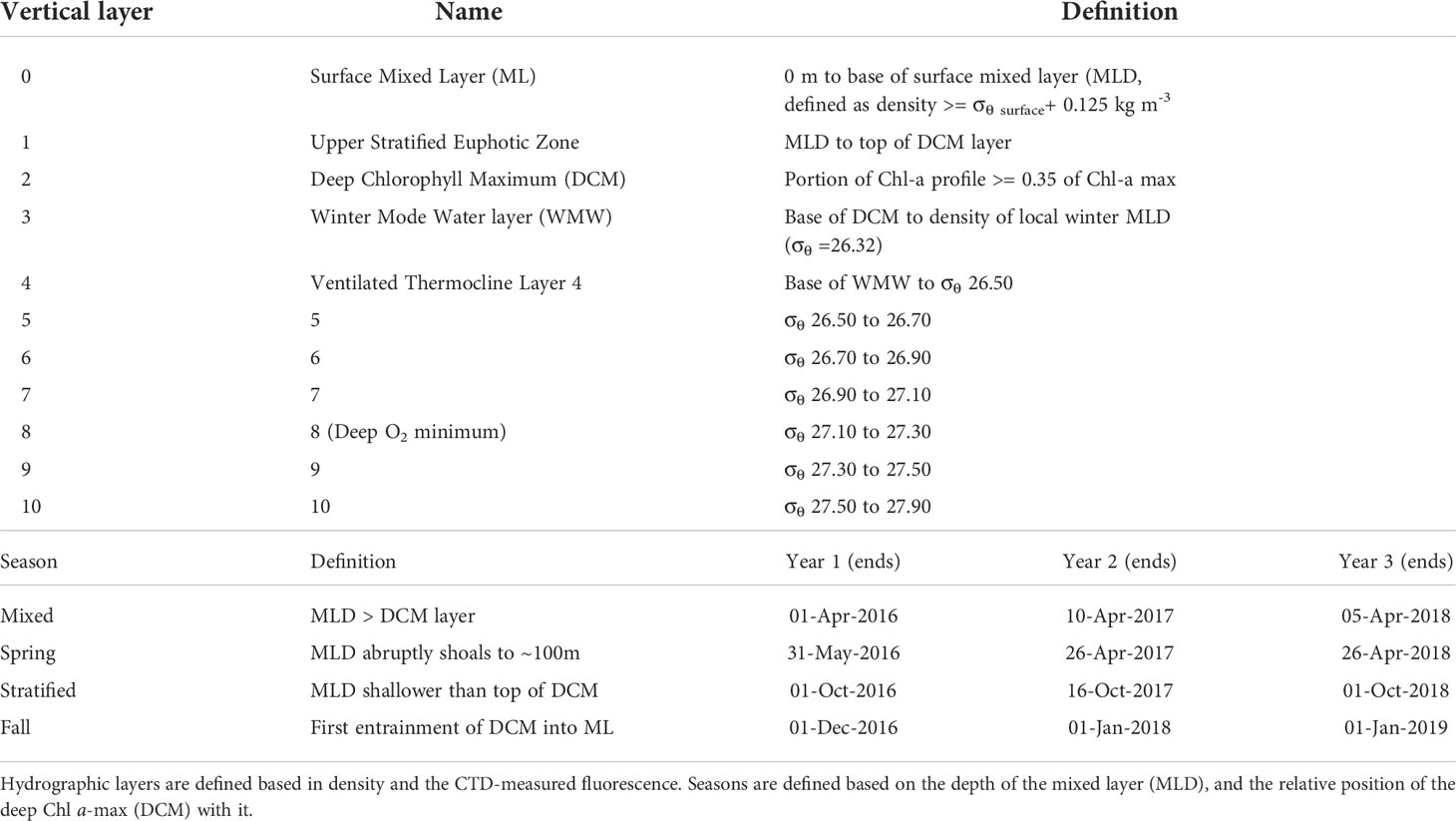
Table 1 Hydrographic envelope for the hydrographic layers and season definitions.
Monthly CTD profiles of temperature, salinity, density, oxygen, and chlorophyll fluorescence paired with discrete bottle sampling, provided hydrographic context. The details of sampling, quality control and post-processing are available on the BATS website (http://bats.bios.edu/index.html). Each profile was assigned to one of four seasons (mixed, spring, stratified, fall; Table 1) based on retrospective evaluation of the full time series for each year. Hydrographic layer boundaries were determined based on a set of pre-defined physical criteria (Table 1) on a profile-by-profile basis from the fluorometer and density criteria.
Biological samples were acquired monthly from February 2016 to December 2018. March 2016 was sampled twice (March 8th and 25th); March 2017 sampling was cancelled due to rough weather. The protocol included 12 fixed depths between surface and 1000 m (0 m, 40 m, 80 m, 120 m, 160 m, 200 m, 250 m, 300 m, 500 m, 600 m, 800 m, 1000 m). At each depth, 4 L of water were filtered using 0.22 µM Sterivex filters (MERCK, MA, USA). Filtering pressure was kept at 5 mmHg. Both ends were sealed with parafilm or a sterile plug/cap. Filters were wrapped in foil and stored at -80°C.
Sucrose lysis buffer (1 mL) was added to the Sterivex filters upon thawing. DNA was extracted using the method by Giovannoni et al. (1990). Amplification and sequencing was carried out in the Center for Genome Research and Biocomputing at Oregon State University. The 18S rRNA V4 hypervariable region was amplified using the primers 5-CCAGCA[GC]C[CT]GCGGTAATTCC-3 and 5-ACTTTCGTTCTTGAT[CT][AG]A-3 (Stoeck et al., 2010), using the KAPA HiFi HotStart ReadyMix (Kapa Biosystems; Wilmington, MA, USA). The PCR thermal cycler program consisted of a 98°C denaturation step for 30 s, followed by 10 cycles of 10 s at 98°C, 30 s at 53°C and 30 s at 72°C, and 15 cycles of 10 s at 98°C, 30 s at 48°C and 30 s at 72°C, and a final elongation step at 72°C for 10 min. After PCR, dual indices and Illumina sequencing adapters were attached using the Illumina Nextera XT Index Kit. Amplicon sequencing was conducted on an Illumina MiSeq using 2x250 PE V2 chemistry.
Quality control and read merging were carried out with MeFiT Ver. 1 (Parikh et al., 2016), using Jellyfish Ver. 2 (Marçais and Kingsford, 2011), with strict parameters to compensate for the lack of complete overlap between forward and reverse: CASPER Ver. 0.8.5 (Kwon et al., 2014) K-mer size of 5, threshold for difference of quality score 5, threshold for mismatching ratio 0.1, and minimum length of overlap of 15. The Merge and Quality Filter Parameters (using the meep score (Koparde et al., 2017)) were set at a filtering threshold of 0.1, discarding non-overlapping reads. Assembled reads passing the QC were fed into MOTHUR ver. 1.43 (Schloss et al., 2009). In short, after trimming to the V4 region (by aligning to the SILVA 138 release trimmed to the V4 region) and removal of chimeras with VSEARCH (Rognes et al., 2016), single variants (=100% OTU; Porter and Hajibabaei, 2018) were obtained using UNOISE2 (Edgar, 2016) as implemented in MOTHUR (diffs=1). Taxonomic assignment was done using the PR2 database (Guillou et al., 2013) using the RDP classifier in MOTHUR. After excluding metazoans and “Eukaryota_unclassified”, samples were rarefied to 20,000 reads and all ASVs with less than two reads (global singletons) were equaled to zero. Scripts are available at the GitHub repository https://github.com/blancobercial/Protist_Time_Series.
Counts per sample and environmental metadata were loaded into PRIMER Ver. 7 (Clarke and Gorley, 2015). Diversity indices (total number of taxa S, Shannon diversity index H’, and Pielou’s evenness index J’) were calculated in PRIMER; Faith’s phylogenetic diversity PD (Faith, 1992) was calculated in MOTHUR using the same input table as for the other indices, after calculating the tree using ClearCut in MOTHUR from the aligned dataset. Samples were then standardize by the total, and square-root transformed (Hellinger transformation) (Legendre and Gallagher, 2001). A Bray-Curtis distance similarity matrix was built, and a Principal Coordinates Analysis (PCoA; Gower, 1966) was carried out. The relationship between environmental variables and the similarity between samples was analyzed with BioEnv in PRIMER, using Spearman Rank and up to five variables for the model. The variables included day of year, depth, temperature, salinity, oxygen, fluorescence, turbidity and density. A second analysis included the factor “hydrographic layer” (Table 1), to assess how this partitioning compared to the protist community. All environmental variables were normalized (subtracting the mean and dividing by the standard deviation) before analyses to remove biases associated to different variable scales.
Non-hierarchical k-means clustering based on group-average ranks was used to find the best grouping reflecting the self-organization of the community, from number of clusters K=2 until two of the clusters were not statistically different (K=14). At each K level, an analysis of similarities (ANOSIM) was run (with 999 permutations) to assess the R-value at each clustering level and if the clustering level was statistically significant (both globally and between pairs of clusters). The K levels showing the maximum R-values were further analyzed. Higher R values (closer to 1) represent higher differences between clusters. Clustering was mapped to the hydrographic layers to assess the fidelity of each community cluster to the pre-defined hydrography-based layering, evaluated within the PCoA ordination, and their taxonomic composition at PR2 “Super-Group” (=Phylum) level analyzed. A test of homogeneity of multivariate dispersions (PERMDISP) was run to compare the dispersion among clusters, as a measure of intra-cluster variability.
The molecular lineages (single variants) with the largest contribution to the similarity in each cluster, and to dissimilarity between adjacent clusters, were assessed using a Similarity Percentage (SIMPER) analyses. Fine taxonomic assignment was done using BLAST (Altschul et al., 1990), analyzing several of the top scores to understand the precision of assignments (species/genus/family/etc.). After selecting the highest scores (and only those with similarity >90%), the lowest shared taxonomy assignment was retained. Interpretation of the seasonal and vertical changes was contextualize within the oceanographic landscape and transitions between clusters, and with the functional profile (based in the literature) of each lineage.
PCoA analyses were further performed at each discrete depth to study the interaction between seasonality and depth. Same procedure was repeated following those samples that overlapped with the Chl-a maximum peak for each profile (which did not happen every month because a set of fixed depths were sampled each time). SIMPER analyses were run to detect taxa related to seasonal succession at each depth.
For all analyses, a Holm-Bonferroni correction was applied to the significance threshold when multiple comparisons were done (Holm, 1979).
Over the 3-year period, hydrographic sampling revealed the expected seasonal cycles of cold season mixing, warm season stratification, the short spring transition, and the vertical distribution of chlorophyll fluorescence (Figure 1). The hydrographic layer boundaries fluctuated in depth over the observational period, highlighting the ability of this physical framework to transcend the temporal variations in vertical water mass structure associated with winter mixing, mesoscale eddies, location of the nutricline, and varying light penetration (Figure 1, Supp. Figure S1). The depth of the surface mixed layer (Layer 0) varied seasonally from 10 m in the stratified season to 170-212 m in the mixed. The depth of the DCM (Deep Chlorophyll Maximum; Layer 2; Figure 1C) ranged from 70 to 130 m. The top of Layer 8, corresponding to the deep O2 minimum (Figure 1B), varied between 600 and 850 m. Other hydrographic features detected were the uplifts in the deep mesopelagic layers due to the passage of large eddies (Figure 1). The most prominent uplifts (of about 200 m) occurred during 2018.
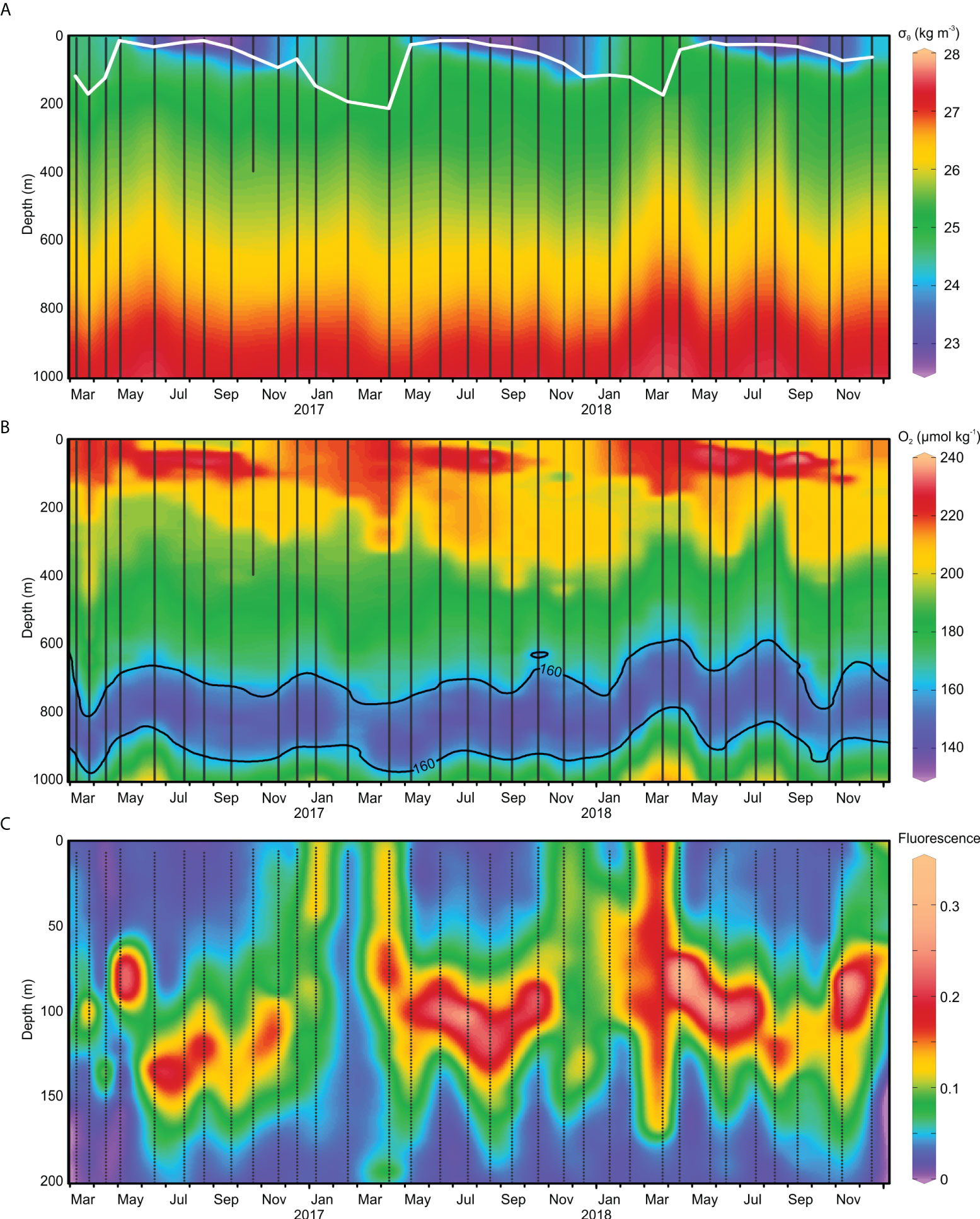
Figure 1 (A) Density (σθ; kg m-3), (B) oxygen (µmol kg-1) and (C) fluorescence (RFU) profiles at BATS station from March 2016 to December 2018. Thin, vertical lines indicate sampling events. Density and oxygen profiles are 0-1000 m, meanwhile fluorescence is shown only in the epipelagic (0-200 m). Mixed Layer Depth (MLD) is indicated by a white line in the density profile. The oxygen minimum zone is defined as the region with less than 160 µmol kg-1, delineated with a black line in the oxygen profile.
Of the 408 samples (34 sampling months, 12 depths), 369 produced a library. The remaining samples failed at some point of the procedure (sampling at sea or extraction), and did not produce a useable library. It usually affected several samples from the same cast, especially the deeper layers (where DNA concentration was always lower). About ~39 million reads were generated (average ~105,000 reads per sample; 23,000 to 364,000). Of those, the strict QC retained 42% as (16.5M reads; 44,000 per sample average) “very high quality” (MEEP definition for those passing the QC settings). There was no link between reads passing QC and months or depths.
Non-hierarchical clustering based on Bray-Curtis distances showed two local R maxima (that is, a maximum in the difference among clusters), for the number of clusters (K) K=2 (ANOSIM R=0.903; p<0.001) and K=9 (R=0.904; p<0.001). These clusters represent groups of samples with similar community composition that are statistically different from the communities in the other clusters. In both cases, all pairwise comparisons between clusters were significant. The K=2 partitioning roughly divided the samples between the epipelagic (photic) and the mesopelagic zones, although when the MLD (Mixed Layer Depth) reached into in the mesopelagic, the upper community followed the MLD depth (Figure 2A). The K=9 clustering aligned closely with the hydrographic layering, with higher numbers of different clusters in the epipelagic, and greater homogeneity in mesopelagic (Figure 2B). In some cases, single clusters spanned several hydrographic layers in the mesopelagic. The clusters precisely traced hydrographic events such as the deepening of the MLD in winter, the abrupt succession to a different community following the shoaling of this layer at the spring transition, and the uplift of mesopelagic layers due to the passage of mesoscale eddies (Figure 2C).
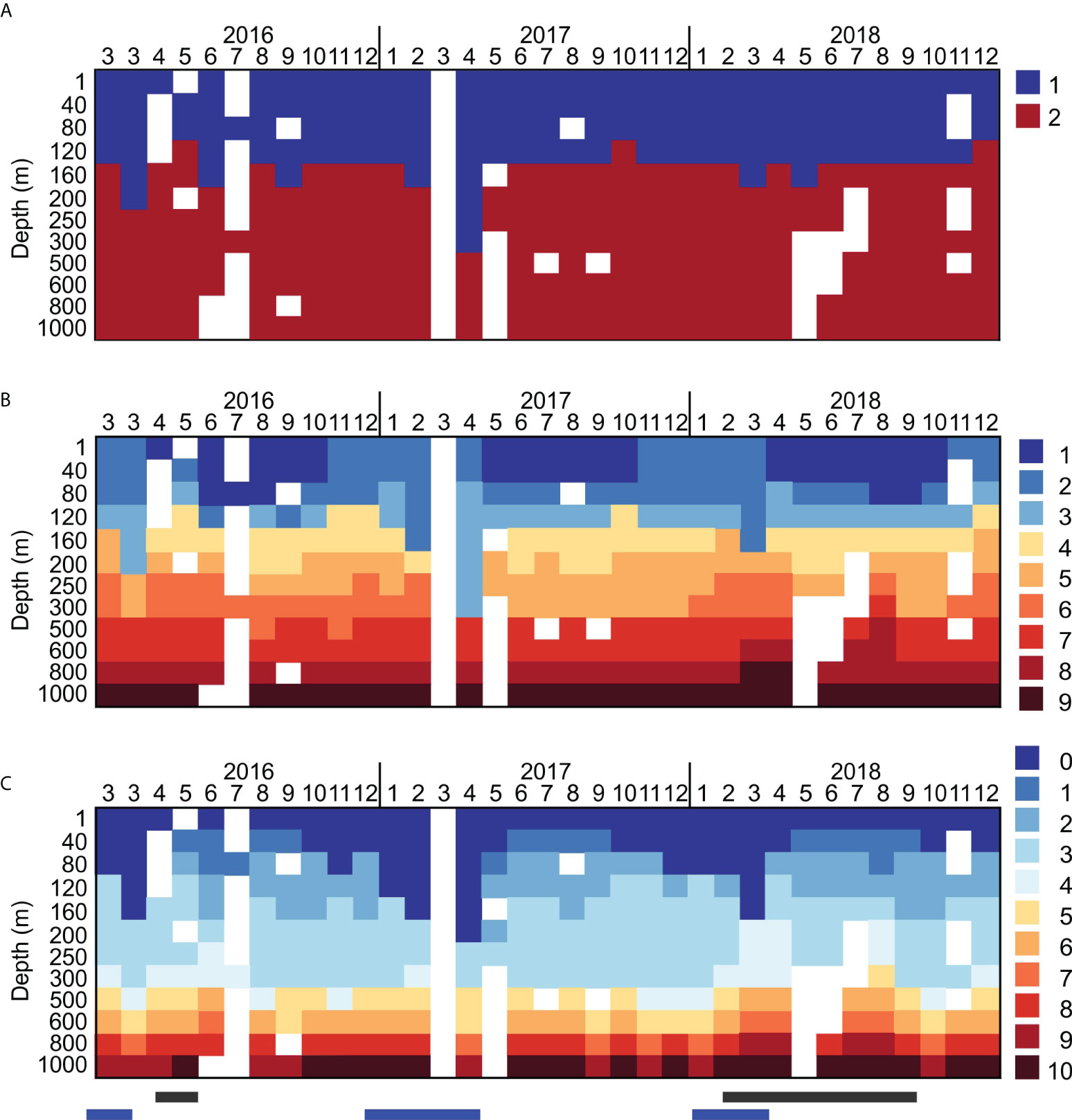
Figure 2 Assignment for each sampled depth, at each month, to the community-composition based on non-hierarchical clusters for (A) K=2 (upper panel) and (B) K=9 (middle panel). Numbers are indicative of months at the top of each panel. K=2 separates the epipelagic and the mesopelagic, meanwhile K=9 reflects the epipelagic seasonality and depth-stratification. The lower panel (C) shows the assignment of each sample to the 11 hydrographic layers defined by Curry et al. (see text, and Table 1). Blue bars correspond to deep mixing events, black bars to uplift of the deeper layers due to the passage of eddies.
In the K=9 grouping (Figure 2B), the epipelagic zone was characterized by a succession of different communities over the annual cycle. Cluster 1 dominated the hydrographic Layer 0 (surface MLD) in the spring and stratified seasons, but was displaced by Cluster 2 during the fall and mixed seasons. Cluster 1 was detected as soon as the MLD shoaled in each year, and remained detectable until the onset of fall when the MLD (Layer 0) gradually deepened and Cluster 2 became dominant. Cluster 3, found below clusters 1 and 2, corresponded to the lower portion of the epipelagic zone that included the DCM (Figures 2A, C). Clusters 4, 5 and 6 occupied the underlying water mass (upper mesopelagic), corresponding to the local deep winter mixed layer (the Winter Mode Water, WMW; Layers 3 & 4), a very weakly stratified portion of the water column occupying the approximate depth range 150-400 m, that did not strictly align with density. Clusters 7, 8 and 9, in the lower mesopelagic (500 – 1000 m), aligned with the density fields. Cluster 8 overlapped with Layer 8, the oxygen minimum zone (OMZ, with O2 < 160 µmol kg-1). The mesopelagic layers were uplifted during the passage of the fronts in 2018, detected by the raised density layers (Figure 2). Clusters were more tightly grouped with depth (PERMDISP test for homogeneity of multivariate dispersions; p < 0.0001), indicating a more variable community in the epipelagic compared to the mesopelagic, and in the upper mesopelagic compared to the deep mesopelagic.
The PCoA ordination arranged the samples with the first axis roughly corresponding to a combination of depth and environmental factors (Figure 3), with many samples departing from their theoretical position if based only on depth (also shown in Figure 2B). The BioEnv procedure determined that the best model to relate the sample ordination with the environmental variables combined O2, fluorescence, depth and density (ρ=0.729 p < 0.001), but since depth and density are highly correlated, the next best model included O2, fluorescence and density (ρ=0.690, p < 0.001). The proposed hydrographic layering was the best-correlated single environmental variable (ρ=0.651, p < 0.001). Superimposing the non-hierarchical clustering onto the PCoA, the K=2 showed a sharp divide between the clusters, despite the intrusions of the upper cluster into deeper layers described before (Figure 1). For K=9, separation of clusters 1 & 2 reflected the seasonal shifts in the upper epipelagic layers (mixed vs stratified conditions). The remaining clusters projected consecutively in the PCoA, with very little mixing at the boundaries. The PCoA also indicated a larger separation between cluster 7 (occupying depths 500 – 600 m) and the other communities. In contrast, clusters 8 (OMZ) and 9 were very close to each other, with minimal mixing.
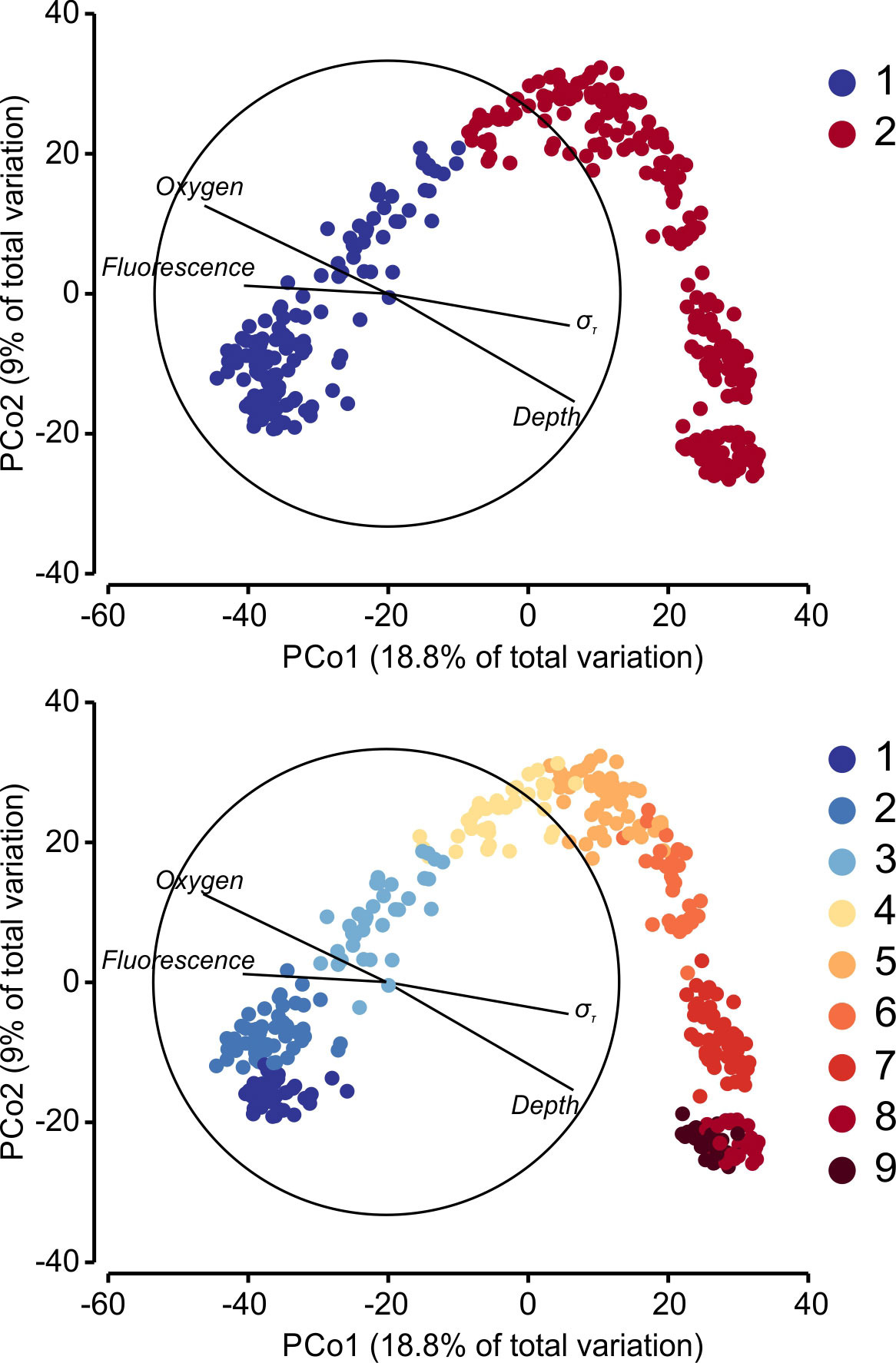
Figure 3 PCoA ordination of all samples for the first two axis, based in their community composition and using Bray-Curtis distances. Environmental factors over are overimposed as vectors, with length corresponding to the correlation ρ. The circle represents ρ=1. Colors indicate the non-hierarchical cluster for each sample, for K=2 (upper panel) and K=9 (lower panel).
The taxonomic composition showed 40-45% of the reads corresponding to Syndiniales (Figure 4), a parasitic group (Guillou et al., 2008); the proportion originating from free dispersal states versus the parasitic state is unknown. At K=2, the taxonomic composition showed a shift from a more diverse community in the epipelagic, with many different clades including autotrophs, heterotrophs and mixotrophs, to a heterotrophic, Rhizaria-dominated, community at depth (Figure 5). This result was more pronounced if the Syndiniales were not considered in the analyses. The variables/single variants with the largest contribution to the similarity within each cluster, identified with the SIMPER analyses, indicated that the epipelagic cluster was characterized by a large presence of autotrophs (mostly Pelagophyceae Pelagomonas calceolata) and mixotrophs (from Ochrophyta, Stramenopiles and Dinophyta) although some of the latter clades include all trophic possibilities. In contrast, heterotrophs overwhelmingly dominated the deep cluster, principally Radiolarians (Polycystinea and Acantharea), and representatives of Stramenopiles (Labyrinthulea). The dissimilarity between groups was then driven by the mixture of autotrophs (especially P. calceolata and the Chlorophyta Ostreococcus sp.) and heterotrophs/mixotrophs (Stramenopiles MAST-4A, and several Dinophyceae lineages) in the epipelagic, compared to their virtual absence in the mesopelagic, where depth-specific heterotrophic Radiolaria dominated.
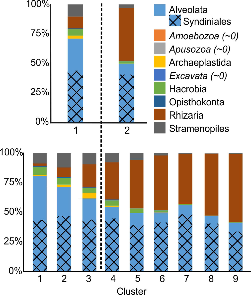
Figure 4 Taxonomic composition (at clade level) for each non-hierarchical cluster at K=2 (top) and K=9 (bottom). The parasitic order Syndiniales is highlighted within the Alveolata, showing its dominance within this phylum. Dashed line approximate the divide between the epi (left) and the mesopelagic (right).
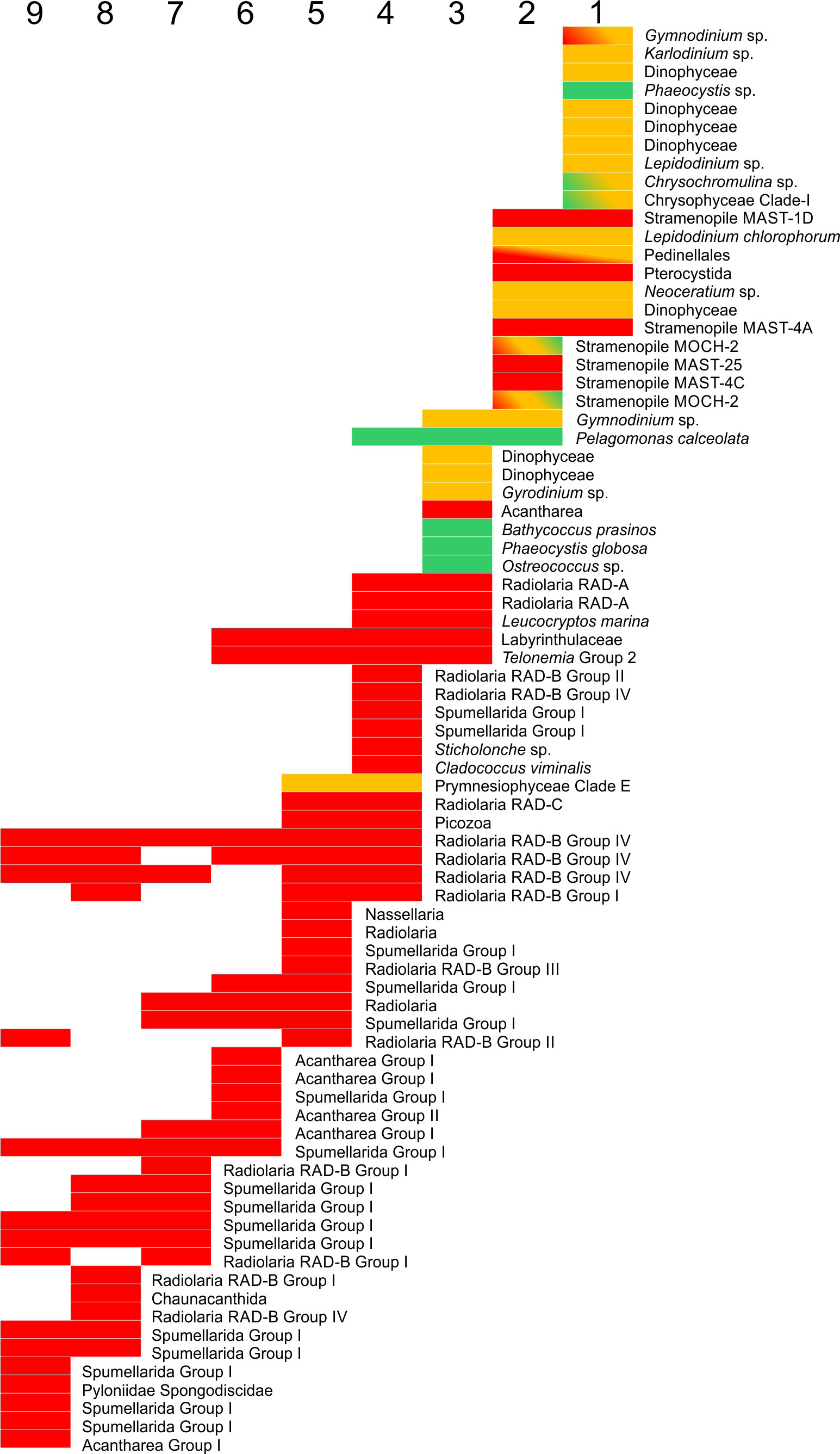
Figure 5 Functional profile (red: heterotroph, orange: mixotroph, green: autotroph) for each of the main components of the nine clusters, as indicated by the SIMPER analyses (after removal of parasitic lineages). When the V4 region was shared among lineages with different functional profiles, the corresponding colors are indicated in the bar.
The taxonomic composition at K=9 reflected a more detailed partitioning (Figure 4). Alveolata dominated the near-surface community during the spring and stratified seasons even if excluding Syndiniales (cluster 1), together with a mixture of Hacrobia and Stramenopiles. In contrast, the near-surface taxa during the mixed periods (cluster 2) exhibited greater abundances of Stramenopiles and Rhizaria. Cluster 3, below clusters 1 & 2, contained the highest concentrations of Archaeplastida, although Rhizaria was the dominant free-living group. A gradual decrease of all the non-Rhizaria groups was associated with increasing depth: Hacrobia and Stramenopiles disappeared almost completely by cluster 7, with only Alveolata maintaining a significant presence. Syndiniales abundances slightly decreased with depth, but had a greater presence in Cluster 7 (500-600 m). SIMPER analyses complimented these findings, determining which taxa showed a clear affinity with cluster. There was no single taxon with a significant presence in all clusters, and most were significant only in one or two clusters. A few Rhizaria, however, showed high numbers in several mesopelagic layers (Figure 5; Table 1). Cluster 1 (surface stratified) was characterized by mixotrophs and heterotrophs of Alveolata Dinophyta (e.g., Warnowia sp., Karlodinium sp. or Lepidodinium spp.), Hacrobia Prymnesiophyceae (Chrysochromulina sp.) and several Stramenopiles. The only autotroph was a clade of Phaeocystis sp., although this group is known to appear as free living or as a symbiont autotroph in Rhizaria colonies. Cluster 2 (near-surface, mixed periods) shows large abundances of P. calceolata (autotroph), but most of the other clades belong to mixotrophs (e.g. several Dinophyceae, and MOCH-2), or heterotrophs (e.g., MAST lineages 25, 4A, 4C and 1D, Hacrobia Pterocystida). Cluster 3 (DCM) showed several mixotrophs among the dominant lineages, but the main groups were autotrophs (the small P. calceolata, Ostreococcus sp., Bathycoccus prasinos, and the Haptophyta Phaeocystis globosa). Heterotrophs characteristic from this clade included the Hacrobia Leucocryptos marina and several Rhizaria (although these might have autotrophic symbionts such as Phaeocytis). Clade 5, below the Chlorophyll maximum, showed significant abundances of the autotroph P. calceolata, however the shift towards a heterotrophic Rhizaria-dominated community was noticeable, together with heterotrophic (Telonemia sp., Leucocryptos marina) and likely mixotrophic (Prymnesiophyceae Clade E) Hacrobia. Different Rhizaria dominated all remaining clusters, while some heterotrophic Hacrobia and Stramenopiles were still among the dominant clades in clusters 5 and 6.
The dissimilarity between consecutive clusters reflected transitions in community function. The mixotroph-dominated cluster one (surface stratified) was replaced by the autotroph-dominated community occupying the ML during the periods of deep mixing (cluster 2). In cluster 3 there was a larger increase of the autotrophs at the cost of mixotrophs from cluster 2. Deeper, differences were due to the progressive decrease in autotrophs, increase of heterotrophs, and layer to layer replacements between different heterotrophs (mostly Rhizaria).
When considering all samples together, there was no discernible seasonal signal. Seasonality, however, appeared when analyzing single depths/clusters. Seasonality was evident in the top layers (surface and 40 m especially; ANOSIM R=0.66 and R=0.62 respectively; p<0.001), but the signal faded with depth, with ANOSIM R progressively decaying (indicating lowering differences among seasons), and becoming non-significant below 300 m. There was no significant seasonality in the mesopelagic. In the lower mesopelagic, the passage of eddies was, however, detectable as a group of dissimilar samples (Figure 6).
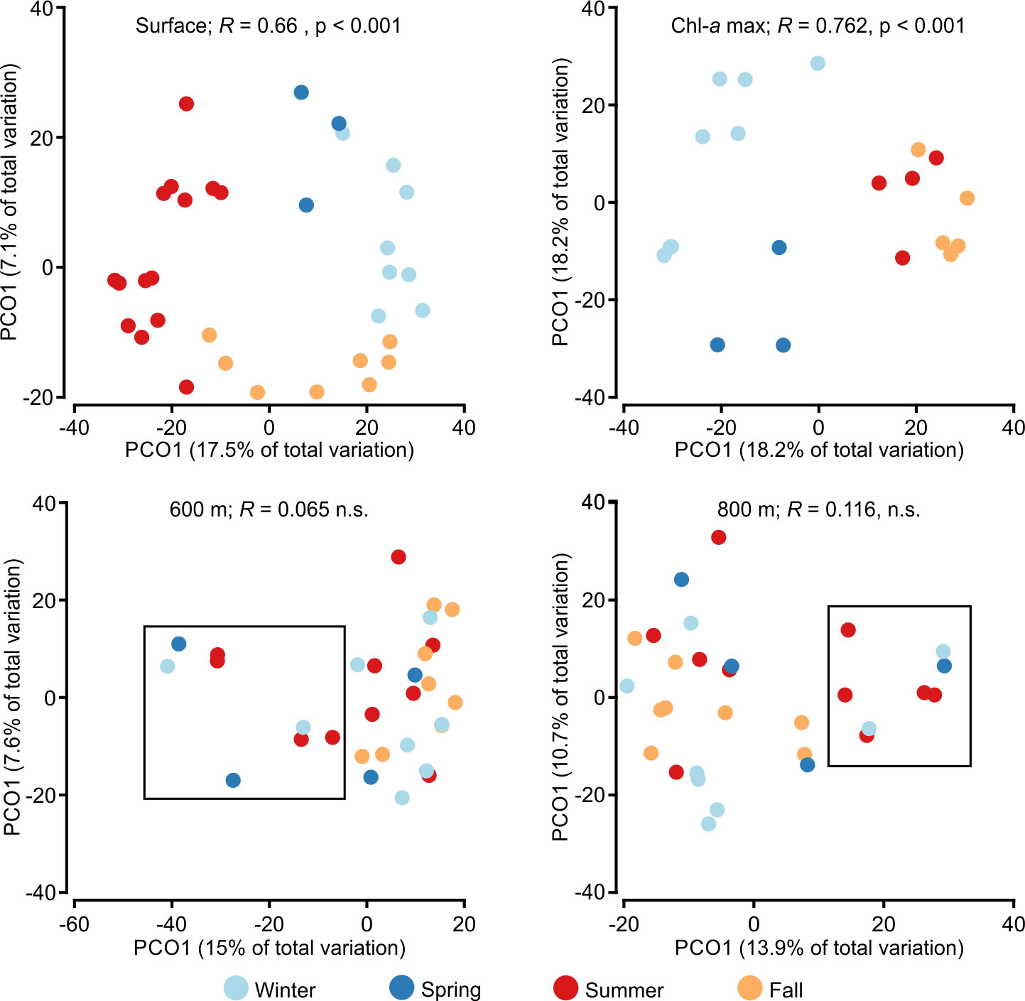
Figure 6 PCoA ordinations for samples from surface (upper left), Chl-a maximum (upper right), 600 m depth (lower left) and 800 m depth (lower right), based in Bray-Curtis distances, with ANOSIM R values for factor “seasons” indicated for each graph, and colors indicating seasons. In the epipelagic, a seasonal signal was detected, especially in the upper layers. In the mesopelagic (lower panels) no seasonality was observed, and samples diverging from the center core at these depths corresponded however to the uplifting events due to the passage of hydrographic features (within the squares).
Near the surface, the highly diverse community was composed of many taxa with low relative abundances (mostly < 2% average), dominated by mixotrophs and heterotroph clades. Only mixed and spring seasons had an autotroph (P. calceolata) among the most abundant clades (only representing ~ 2% of the reads), while a single heterotroph identified as Warnowia sp. represented 8% of reads in spring. In the stratified season, mixotrophs, and a diverse community of heterotrophs, including Telonemia, Warnowia, several Hacrobia Centroheliozoa and the Rhizaria Minorisa minuta dominated the community. In the fall, mixotrophs gained more prominence compared to heterotrophs.
Cluster 3 was generally associated with the Layer 2 (broadly defined DCM) but, since the DCM varied substantially, sometimes this layer did not capture the feature. Cluster 3 community exhibited depth dependence, but no apparent seasonal cycle. When DCM samples were restricted to those acquired within 90% of the actual chlorophyll maximum, a strong and significant seasonal pattern was detected (ANOSIM R = 0.762, p < 0.001; Figure 6). The stratified and fall periods, despite mixing in the 2PCos representation, were statistically different (R = 0.5, p < 0.05) and were separated in the 3-PCoA (Figure S2). The SIMPER analyses performed to find the main contributors to the dissimilarity between these seasons in this narrow Chl-a max, showed that the main difference happened during the spring season, when a few autotrophic clades dominate the community (Ostreococcus sp., P. calceolata and B. prasinos). Three different clades of Micromonas, and P. globosa, were also among the most abundant clades. Together, autotrophs represented over 30% of the reads of the non-parasitic community. Other main groups included Dinophyceae (likely mixotrophs) and heterotrophs such as Telonemia sp. and Radiolaria (although these might have autotrophic endosymbionts). After transitioning to the stratified period, only P. calceolata, B. prasinos and P. globosa showed relatively high abundances in the DCM; however, their prevalence was much lower (just above 5%). In contrast, mixotrophs and heterotrophs increased in relative abundance. In the fall transition, P. calceolata and P. globosa were the only autotrophs among the main taxa (with slightly higher relative abundances compared to the stratified period), while the proportion of heterotrophs (Rhizaria and Telonemia) increased. During the mixing season, there was again a strong shift to autotrophs (especially P. calceolata, B. prasinus and Ostreococcus. sp.; about 10% of the total reads combined) and mixotrophs, with no free heterotrophs among the main lineages in the community.
Diversity indices indicated a mismatch between species-based and phylogenetic-based diversity indices (Figure 7). The data showed a higher number of species (S), species diversity (H’) and evenness (J’) in the upper layers of the water column, gradually decreasing with depth, reaching a minimum in the cluster corresponding to the oxygen minimum zone. These profiles also revealed an interesting feature: superimposed upon the general trend of decreasing diversity and evenness with increasing depth throughout the upper 1000 m, the indices identified three subgroups (clusters 1-3, 4-6 and 7-9) each of which exhibited its own decreasing trend. The subgroups correspond respectively to the epipelagic, upper mesopelagic, and lower mesopelagic portions of the water column. The profile for Faith’s phylogenetic diversity was distinctly different from these: it showed rising diversity from clusters 1 to 4, followed by a steady decrease with depth to a minimum in the OMZ.
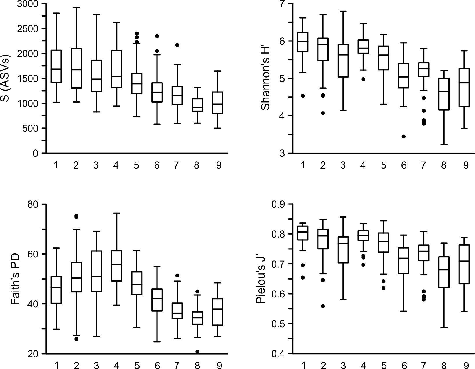
Figure 7 Box and whiskers graphs for the distribution of the number of taxa (S), Shannon’s H’, Faith PD and Pielou’s J’ for all samples from each cluster at K=9. Boxes indicate median, first and third quartiles. Meanwhile S and H’ follow a decreasing pattern with depth, PD shows a maxima at cluster 4 (below the DCM), and Pielou’s J’ shows three different decreasing trends, in the epipelagic, and the upper and lower mesopelagic.
The data presented here supports the presence of a significant seasonality in the photic community in the Subtropical North Atlantic, whose signal and strength gradually decreases with depth, becoming undetectable in the mesopelagic. The structure of epipelagic and mesopelagic protist communities in the Sargasso Sea is strongly shaped by local ocean dynamics (e.g., mixing, stratification, nutrient distributions and light penetration) and expressed in the vertical and seasonal partitioning of community composition, diversity, and function. Mixotrophic groups dominate the sunlit epipelagic layers, with small, autotrophic taxa gaining relevance where the base of the photic layer meets the top of the nutricline (Arenovski et al., 1995). The mesopelagic layers below are inhabited by heterotrophic communities where Rhizaria becomes the most abundant group, outside of parasitic lineages (i.e. Syndiniales). The deep communities are likely fueled by complex food webs, feeding on prokaryotes, particles and each other (Byung Cheol et al., 2000; Rocke et al., 2015). With the present warming trends, favoring cyanobacteria at the expenses of the eukaryotic community, especially during the stratification periods (Lomas et al., 2022), it is essential to characterize the present communities to understand futures changes in composition and functionality, their seasonal successions, and their vertical arrangement in the water column.
Nutrient limitation in the epipelagic zone favors mixo- and heterotrophic protists closer to the surface, with autotrophs balancing nutrients and light at its base. This is largely a consequence of ocean stratification, which enhances or inhibits vertical exchanges. The degree of stratification at the base of the photic zone affects the rate of nutrient supply fueling the autotrophic lineages at the local DCM. Over the annual cycle, hydrographic Layers 0, 1 and 2 exhibit dramatic changes in stratification driven by local air-sea fluxes, with hydrographic layers 1 and 2 being subsumed into layer 0 beginning in the Fall and ending at the Spring transition. This process creates the vertical partitioning of community clusters 1, 2 and 3 and their seasonality observed in K=9: i.e. clusters 1 and 2 dominate hydrographic layers 0 and 1 above the DCM from Spring through the Stratified season, with cluster 1 disappearing in the Fall and Mixed seasons. Cluster 3, in hydrographic layer 2, waxes in Spring then gradually wanes through the Stratified and Fall seasons. Such seasonality is absent at ALOHA in the North Pacific where winter mixing is shallower, the base of the photic layer remains stratified throughout the year, and protist communities align with depth (Ollison et al., 2021). This difference is not unexpected, due to the more constant hydrographic conditions, primary production and particle flux measured throughout the year by the Hawaii Ocean Time-series compared to those at BATS (Church et al., 2013). The more homogeneous conditions would then favor the presence of a dominant community all year long at ALOHA, showing only depth-controlled layering.
The pronounced seasonality observed in the Sargasso Sea implies shifts in trophic ecology and energy fluxes which likely influence biogeochemical cycles over the annual cycle (Goericke, 1998; Lomas et al., 2013). High relative abundances of mixotrophs and heterotrophs compared to autotrophs during the stratified and fall seasons indicate a complex recycling food web where small protists such as Warnowia, Telonemia, Karlodinium or Minorisa minuta and MAST and MOCH lineages prey on picophytoplankton, responsible of most of the primary production in the Sargasso Sea (Caron et al., 1999; Sanders et al., 2000; Klaveness et al., 2005; Riemann et al., 2011; Place et al., 2012; del Campo et al., 2013; Massana et al., 2014; Orsi et al., 2018; Cotti-Rausch et al., 2020). Both autotrophs and small mixo- and heterotrophs would also be preyed upon by larger mixotrophs or heterotrophs protists (Lessard and Murrell, 1998; Quevedo and Anadón, 2001; Andersen et al., 2011). Autotrophic protists (picophytoplankton and small nanophytoplankton, such as Ostreococcus, Bathycoccus or Pelagomonas calceolata) had a numerical relevance only in the mixed and spring seasons, but mixotrophs still represent a significant portion of the community. Those mixotrophs would benefit from their ability to carry out photosynthesis, while still preying on the small autotrophs (Sanders et al., 2000), likely due to the concurring C fixation by photosynthesis with the heterotrophic acquisition of N and P (Edwards, 2019). Recently, Choi et al. (2020) reported elevated summer abundances of uncultured dictyophytes at BATS, and evidence that these taxa are more prevalent in the upper water common when nutrients are most depleted. These and other observations, and the findings we report, suggest that mixotrophic strategies become relatively more advantageous when production is limited by macronutrients, likely due to the repartitioning of N and P rather than the energetic benefits of mixotrophy. As such, in the oligotrophic Sargasso Sea they would be at a significant advantage compared to non-mixotrophs (Duhamel et al., 2019; Edwards, 2019; Choi et al., 2020), only attenuated during the strong mixing period. Shifting between mixotrophy-dominated and autotrophy-dominated communities has implications in nutrient cycling (in terms of e.g. sources, metabolic byproducts or remineralization of those) and trophic structure of the community (Mitra et al., 2016; Cohen, 2022).
The observed month-to-month depth expansion and contraction of the different protist communities influences community functionality. Cluster 1, which occupies the near surface layers throughout the spring and stratified season, disappears in fall when the surface MLD begins to erode into the DCM, and only emerges again when the ML abruptly shoals the following spring. The temporary nature of this group contrasts with the other communities, which are likely present throughout the year, albeit with periods of expansion and contraction. As such, heterotrophy, and its trophic and biogeochemical consequences, would increase in summer and fall, with the expansion of the stratified surface community. The fall is also when the Chl-a-max corresponds to a community rich in heterotrophs, although many are potential mixotrophs via endosymbionts (Bjorbækmo et al., 2020). The effect of these non-constitutive mixotrophs on the biogeochemical cycles is one major question to be addressed in the future. Although in some cases a few clusters are missing in some months, it might be an artifact of the punctuated depth sampling with niskin bottles, which would miss their depths at that particular month. As a comparison, the bottle sampling also missed some of the density-derived layers, but they were all present in the continuous profiles. In those months, some of the deeper clusters were then missed.
It should be noted that in some cases the functionality of taxa is relatively easy to assign (e.g. Telonemia or Ostreococcus), while in many other cases it is difficult to assess with certainty. Close relatives, with different functional profiles (i.e. mixotrophy vs. autotrophy) often share a single V4 sequence. Other sources of uncertainty come from the non-constitutive mixotrophs. In our case, the main group is Rhizaria. These are known to potentially carry photosynthetic endosymbionts (e.g., Phaeocystis sp.) (Bjorbækmo et al., 2020). Addressing these uncertainties is required to understand the full role of mixotrophy in the oceans, and its influence in the biogeochemical cycles (Mitra et al., 2014; Gonçalves Leles et al., 2018; Edwards, 2019; Flynn et al., 2019; Gonçalves Leles et al., 2021).
In the mesopelagic zone, protist are vertically partitioned into distinct communities that occupy specific density strata. This may reflect a response to resource availability and/or particular environmental conditions (Biard and Ohman, 2020), such as the OMZ, where there is an increase in particles. Within the main clades, specific lineages also occupied specific hydrographic layers, suggesting a preferred niche for each, similarly to what was observed in the Rhizaria. An alternate explanation is that vertical biological gradients may reflect “where” and “when” the density layers were at the sea surface - i.e. the ventilated thermocline model of gyre circulation (Luyten et al., 1983). The “age” of a water parcel at BATS typically increases with depth/density reflecting longer distances traveled since ventilation. Geographic gradients in surface community composition could thus translate to vertical gradients at mesopelagic depths, and/or, if the community composition evolves as a function of time, the vertical gradients may reflect “age”.
Our findings, showing higher diversity in the epipelagic, peaking below the Chl-a max, and then decreasing with depth, are opposite in pattern to the study by Ollison et al. (2021). These differences can be attributed to many causes. There is great disparity in the environmental conditions, with strong seasonality and fully oxic OMZ at BATS compared to the quasi-permanent conditions and the thick and suboxic OMZ at ALOHA (Church et al., 2013). Additionally there are pure methodological differences: the present manuscript is based on DNA metabarcoding, while Ollison et al. (Ollison et al., 2021) used an RNA-based metabarcoding approach. Our data, however, coincides with the findings of Canals et al. (2020), where a similar pattern of decreasing diversity with depth and a peak around the Chl-a maximum, was found for ciliates in the Atlantic Ocean, suggesting that the environmental landscape (the hydrography) is driving the differences between ocean basins.
The clear signal of increasing phylogenetic diversity towards the Chl-a-max, with the layers below the 1% (but above the mesopelagic) showing the highest diversity, is notable. This maxima might be related to the presence of more, and more diverse, ecological niches, since here light and nutrients are able to sustain a rich autotroph community (below it is too dark; nutrients are scarce above) in addition to the heterotroph and mixotrophs, facilitating the coexistence of more phylogenetically apart lineages. This pattern contrasts with the taxonomic diversity, either H’, or SVs richness, which did not show a noticeable change in the epipelagic. This mismatch is significant since PD is often directly correlated to species richness (Barker, 2008; Voskamp et al., 2020). The pattern here likely reflects the abrupt transition from an Alveolata-dominate surface community towards one more phylogenetically diverse, despite a relatively constant species richness, owing to the availability of nutrients.
The mesopelagic communities exhibited lower diversity and tighter grouping in the PCoA, indicative of less month-to-month variability compared to epipelagic communities. These patterns may be related to seasonality in the epipelagic layers, where a more dynamic environment would favor community succession processes month to month (represented as a higher dispersal between samples) and inhibits efficient competitive exclusion processes (causing higher diversity within sample). The deeper layers, however, characterized by less environmental variability, would favor the same lineages with competitive advantages month after month, limiting the number of taxa, and resulting in more stable communities. The vertical stratification of the Rhizaria community could be due to resource availability (decreasing with depth; Pedrosa-Pàmies et al., 2018), resource structure (e.g. presence and size of aggregates, filaments, or dissolved) and/or elemental stoichiometry with depth.
Metabarcoding approaches, as any other method, are subject to many methodological limitations and bias (Bucklin et al., 2016; Santoferrara, 2019). The initial selection of which region and primers to use, the marker copy number variability between taxa, etc., are a source of biases that would affect the description of the community. Other source of uncertainty is the taxonomic assignment of the different lineages (SV or OTUs), due to both incomplete databases (where there is a lot of work to do by the community), and to the lack of resolution at the species level by most ribosomal markers. To mitigate these biases, the taxonomy for the discussed lineages was analyzed against GenBank, to understand the ambiguity of the taxonomic assignment, and corrected if needed (compared to the mothur PR2 based assignment). Regarding the copy number bias, we are confident that the core of this manuscript, the seasonal and depth community transitions, are not affected by this fact, since there are strong changes in the community composition and not small changes of the same taxa, and would very likely hold true independently of the marker used. Finally, the raw value of the diversity indices should be considered only in the context of this study, since methodological questions as the indicated or the rarefaction (or extrapolation) level chosen can drastically affect diversity estimates (Santoferrara, 2019; Blanco-Bercial, 2020). Despite this possible bias, it is very likely that the observed patterns of variability (where diversity is higher/lower, etc.) are however robust against those bias. Any comparison with other existing data would require a reanalysis with shared bioinformatics approaches.
The protist community in the Sargasso Sea shows a dynamic seasonality in the epipelagic, responding to hydrographic yearly cycles. Mixotrophic lineages, able to take advantage of the smaller picophytoplankton and heterotroph bacterioplankton, dominate throughout the year; however, autotrophs bloom during the rapid transition between the winter mixing and the stratified summer. Pure heterotrophs have their peak moment at the end of summer, when the base of the thermocline reaches its deepest depth, and likely mixotrophs lose part of their photosynthetic advantage due to the almost complete depletion of nutrients near the surface. Below the photic zone, the community, dominated by Rhizaria, is depth-stratified, relatively constant throughout the year. These populations, relying on the vertical flux of organic matter, respond to local hydrographic and biological features such as the oxygen minimum zone. Together, this suggests a dynamic partitioning of the water column, where the niche vertical position for each community changes throughout the year, likely depending on nutrient availability, the mixed layer depth, and other hydrographic features. Future research should address several uncertainties needed to implement these data into biogeochemical models. The most prominent problem to solve is the lack of lineage-level quantitative data (i.e., counts), which would allow a better understanding of the energy flows. Most of the lineages we report on here are 2-20 µm in cell diameter, falling in the range where taxon-specific cell counting is most difficult, between flow cytometry and automated image analyses. A second uncertainty is clarifying the functionality (trophic modes) in those lineages (e.g. MOCH groups with autotrophs, mixotrophs, and heterotrophs), to more accurately associate these strategies with the temporal and spatial patterns in the system. Together with the present data, these would allow better characterization of the carbon flux throughout the water column, and the role of mixotrophs and heterotrophs in controlling the biogeochemical cycles in the oligotrophic oceans.
The data presented in the study are deposited in the NCBI repository, accession number PRJNA769790.
LB-B conceived the experiment. RP, LB, RJ, and RC acquired the samples and/or conducted the experiments. LB-B and RC analyzed the samples. LB-B wrote the manuscript with contributions and review by all authors. All authors contributed to the article and approved the submitted version.
This research was funded by the Simon’s Foundation International as part of the BIOSSCOPE (http://scope.bios.edu/) and MAGIC (SFI award #545298) projects, the NSF funded OCE-1851224, and the Bermuda Atlantic Time-series Study program (BATS; NSF OCE-1756105).
Special thanks to the BATS personnel and to the Captains and crew of the RV Atlantic Explorer for their logistical support at sea. This research made use of the FCMMF laboratory equipment at BIOS (NSF DBI-1522206).
The authors declare that the research was conducted in the absence of any commercial or financial relationships that could be construed as a potential conflict of interest.
The reviewer SW declared a past co-authorship with the author SG to the handling editor.
All claims expressed in this article are solely those of the authors and do not necessarily represent those of their affiliated organizations, or those of the publisher, the editors and the reviewers. Any product that may be evaluated in this article, or claim that may be made by its manufacturer, is not guaranteed or endorsed by the publisher.
The Supplementary Material for this article can be found online at: https://www.frontiersin.org/articles/10.3389/fmars.2022.897140/full#supplementary-material
Agusti S., Lubián L. M., Moreno-Ostos E., Estrada M., Duarte C. M. (2019). Projected changes in photosynthetic picoplankton in a warmer subtropical ocean. Front. Mar. Sci. 5 (506). doi: 10.3389/fmars.2018.00506
Altschul S. F., Gish W., Miller W., Myers E. W., Lipman D. J. (1990). Basic local alignment search tool. J. Mol. Biol. 215 (3), 403–410. doi: 10.1016/S0022-2836(05)80360-2
Amaral-Zettler L. A., McCliment E. A., Ducklow H. W., Huse S. M. (2009). A method for studying protistan diversity using massively parallel sequencing of V9 hypervariable regions of small-subunit ribosomal RNA genes. PLoS One 4 (7), e6372. doi: 10.1371/annotation/50c43133-0df5-4b8b-8975-8cc37d4f2f26
Andersen N. G., Nielsen T. G., Jakobsen H. H., Munk P., Riemann L. (2011). Distribution and production of plankton communities in the subtropical convergence zone of the Sargasso Sea II. Protozooplankton and copepods. Mar. Ecol. Prog. Ser. 426, 71–86. doi: 10.3354/meps09047
Arenovski A. L., Lim E. L., Caron D. A. (1995). Mixotrophic nanoplankton in oligotrophic surface waters of the Sargasso Sea may employ phagotrophy to obtain major nutrients. J. Plankton Res. 17 (4), 801–820. doi: 10.1093/plankt/17.4.801
Barker G. M. (2008). Phylogenetic diversity: a quantitative framework for measurement of priority and achievement in biodiversity conservation. Biol. J. Linn. Soc. 76 (2), 165–194. doi: 10.1111/j.1095-8312.2002.tb02081.x
Biard T., Ohman M. D. (2020). Vertical niche definition of test-bearing protists (Rhizaria) into the twilight zone revealed by in situ imaging. Limnol Oceanog 65 (11), 2583–2602. doi: 10.1002/lno.11472
Bjorbækmo M. F. M., Evenstad A., Røsæg L. L., Krabberød A. K., Logares R. (2020). The planktonic protist interactome: where do we stand after a century of research? ISME J. 14 (2), 544–559. doi: 10.1038/s41396-019-0542-5
Blanco-Bercial L. (2020). Metabarcoding analyses and seasonality of the zooplankton community at BATS. Front. Mar. Sci. 7 (173). doi: 10.3389/fmars.2020.00173
Bucklin A., Lindeque P. K., Rodriguez-Ezpeleta N., Albaina A., Lehtiniemi M. (2016). Metabarcoding of marine zooplankton: prospects, progress and pitfalls. J. Plankton Res. 38 (3), 393–400. doi: 10.1093/plankt/fbw023
Byung Cheol C., Sang Cheol N., Dong Han C. (2000). Active ingestion of fluorescently labeled bacteria by mesopelagic heterotrophic nanoflagellates in the East Sea, Korea. Mar. Ecol. Prog. Ser. 206, 23–32. doi: 10.3354/meps206023
Calbet A., Landry M. R. (2004). Phytoplankton growth, microzooplankton grazing, and carbon cycling in marine systems. Limnol Oceanog 49 (1), 51–57. doi: 10.4319/lo.2004.49.1.0051
Canals O., Obiol A., Muhovic I., Vaqué D., Massana R. (2020). Ciliate diversity and distribution across horizontal and vertical scales in the open ocean. Mol. Ecol. 29 (15), 2824–2839. doi: 10.1111/mec.15528
Caron D. A., Hu S. K. (2019). Are we overestimating protistan diversity in nature? Trends Microbiol. 27 (3), 197–205. doi: 10.1016/j.tim.2018.10.009
Caron D. A., Peele E. R., Lim E. L., Dennett M. R. (1999). Picoplankton and nanoplankton and their trophic coupling in surface waters of the Sargasso Sea south of Bermuda. Limnol Oceanog 44 (2), 259–272. doi: 10.4319/lo.1999.44.2.0259
Choi C. J., Jimenez V., Needham D. M., Poirier C., Bachy C., Alexander H., et al. (2020). Seasonal and geographical transitions in eukaryotic phytoplankton community structure in the Atlantic and pacific oceans. Front. Microbiol. 11 (2187). doi: 10.3389/fmicb.2020.542372
Church M. J., Lomas M. W., Muller-Karger F. (2013). Sea Change: Charting the course for biogeochemical ocean time-series research in a new millennium. Deep Sea Res. Part II: Topical Stud. Oceanog 93, 2–15. doi: 10.1016/j.dsr2.2013.01.035
Cohen N. R. (2022). Mixotrophic plankton foraging behaviour linked to carbon export. Nat. Commun. 13 (1) 1302. doi: 10.1038/s41467-022-28868-7
Conte M. H., Ralph N., Ross E. H. (2001). Seasonal and interannual variability in deep ocean particle fluxes at the oceanic flux program (OFP)/Bermuda Atlantic time series (BATS) site in the western Sargasso Sea near Bermuda. Deep Sea Res. Part II: Topical Stud. Oceanog 48 (8), 1471–1505. doi: 10.1016/S0967-0645(00)00150-8
Cotti-Rausch B. E., Lomas M. W., Lachenmyer E. M., Baumann E. G., Richardson T. L. (2020). Size-fractionated biomass and primary productivity of Sargasso Sea phytoplankton. Deep Sea Res. Part I: Oceanog Res. Papers 156, 103141. doi: 10.1016/j.dsr.2019.103141
del Campo J., Not F., Forn I., Sieracki M. E., Massana R. (2013). Taming the smallest predators of the oceans. ISME J. 7 (2), 351–358. doi: 10.1038/ismej.2012.85
de Vargas C., Audic S., Henry N., Decelle J., Mahé F., Logares R., et al. (2015). Eukaryotic plankton diversity in the sunlit ocean. Science 348 (6237). doi: 10.1126/science.1261605
Duhamel S., Kim E., Sprung B., Anderson O. R. (2019). Small pigmented eukaryotes play a major role in carbon cycling in the P-depleted western subtropical north Atlantic, which may be supported by mixotrophy. Limnol Oceanog 64 (6), 2424–2440. doi: 10.1002/lno.11193
Edgar R. C. (2016). UNOISE2: improved error-correction for illumina 16S and ITS amplicon sequencing. BioRxiv 081257. doi: 10.1101/081257
Edwards K. F. (2019). Mixotrophy in nanoflagellates across environmental gradients in the ocean. Proc. Natl. Acad. Sci. 116 (13), 6211–6220. doi: 10.1073/pnas.1814860116
Faith D. P. (1992). Conservation evaluation and phylogenetic diversity. Biol. Conserv. 61 (1), 1–10. doi: 10.1016/0006-3207(92)91201-3
Flynn K. J., Mitra A., Anestis K., Anschütz A. A., Calbet A., Ferreira G. D., et al. (2019). Mixotrophic protists and a new paradigm for marine ecology: where does plankton research go now? J. Plankton Res. 41 (4), 375–391. doi: 10.1093/plankt/fbz026
Giovannoni S. J., DeLong D. F., Schmidt T. M., Pace N. R. (1990). Tangential flow filtration and preliminary phylogenetic analysis of marine picoplankton. Appl. Environ. Microbiol. 56, 2572–2575. doi: 10.1128/aem.56.8.2572-2575.1990
Goericke R. (1998). Response of phytoplankton community structure and taxon-specific growth rates to seasonally varying physical forcing in the Sargasso Sea off Bermuda. Limnol Oceanog 43 (5), 921–935. doi: 10.4319/lo.1998.43.5.0921
Gonçalves Leles S., Bruggeman J., Polimene L., Blackford J., Flynn K. J., Mitra A. (2021). Differences in physiology explain succession of mixoplankton functional types and affect carbon fluxes in temperate seas. Prog. Oceanog 190, 102481. doi: 10.1016/j.pocean.2020.102481
Gonçalves Leles S., Polimene L., Bruggeman J., Blackford J., Ciavatta S., Mitra A., et al. (2018). Modelling mixotrophic functional diversity and implications for ecosystem function. J. Plankton Res. 40 (6), 627–642. doi: 10.1093/plankt/fby044
Gower J. C. (1966). Some distance properties of latent root and vector methods used in multivariate analysis. Biometrika 53 (3-4), 325–338. doi: 10.1093/biomet/53.3-4.325
Guillou L., Bachar D., Audic S., Bass D., Berney C., Bittner L., et al. (2013). The protist ribosomal reference database (PR2): a catalog of unicellular eukaryote small Sub-unit rRNA sequences with curated taxonomy. Nucleic Acids Res. 41 (D1), D597–D604. doi: 10.1093/nar/gks1160
Guillou L., Viprey M., Chambouvet A., Welsh R. M., Kirkham A. R., Massana R., et al. (2008). Widespread occurrence and genetic diversity of marine parasitoids belonging to syndiniales (Alveolata). Environ. Microbiol. 10 (12), 3349–3365. doi: 10.1111/j.1462-2920.2008.01731.x
Holm S. (1979). A simple sequentially rejective multiple test procedure. Scandinavian J. Stat 6 (2), 65–70.
Irwin A. J., Oliver M. J. (2009). Are ocean deserts getting larger? Geophys Res. Lett. 36 (18). doi: 10.1029/2009GL039883
Klaveness D., Shalchian-Tabrizi K., Thomsen H. A., Eikrem W., Jakobsen K. S. (2005). Telonema antarcticum sp. nov., a common marine phagotrophic flagellate. Int. J. Systematic Evolutionary Microbiol. 55 (6), 2595–2604. doi: 10.1099/ijs.0.63652-0
Koparde V. N., Parikh H. I., Bradley S. P., Sheth N. U. (2017). MEEPTOOLS: a maximum expected error based FASTQ read filtering and trimming toolkit. Int. J. Comput. Biol. Drug Design 10 (3), 237–247. doi: 10.1504/ijcbdd.2017.085409
Kwon S., Lee B., Yoon S. (2014). CASPER: context-aware scheme for paired-end reads from high-throughput amplicon sequencing. BMC Bioinf. 15 (9), S10. doi: 10.1186/1471-2105-15-S9-S10
Latorre F., Deutschmann I. M., Labarre A., Obiol A., Krabberød A. K., Pelletier E., et al. (2021). Niche adaptation promoted the evolutionary diversification of tiny ocean predators. Proc. Natl. Acad. Sci. 118 (25), e2020955118. doi: 10.1073/pnas.2020955118
Legendre P., Gallagher E. D. (2001). Ecologically meaningful transformations for ordination of species data. Oecologia 129 (2), 271–280. doi: 10.1007/s004420100716
Lessard E. J., Murrell M. C. (1998). Microzooplankton herbivory and phytoplankton growth in the northwestern Sargasso Sea. Aquat. Microbial. Ecol. 16 (2), 173–188. doi: 10.3354/ame016173
Lomas M. W., Bates N. R., Johnson R. J., Knap A. H., Steinberg D. K., Carlson C. A. (2013). Two decades and counting: 24-years of sustained open ocean biogeochemical measurements in the Sargasso Sea. Deep Sea Res. Part II: Topical Stud. Oceanog 93 (0), 16–32. doi: 10.1016/j.dsr2.2013.01.008
Lomas M. W., Bates N. R., Johnson R. J., Steinberg D. K., Tanioka T. (2022). Adaptive carbon export response to warming in the Sargasso Sea. Nat. Commun. 13 (1) 1211. doi: 10.1038/s41467-022-28842-3
Luyten J., Pedlosky J., Stommel H. (1983). The ventilated thermocline. J. Phys. Oceanog 13 (2), 292–309. doi: 10.1175/1520-0485(1983)013<0292:TVT>2.0.CO;2
Marçais G., Kingsford C. (2011). A fast, lock-free approach for efficient parallel counting of occurrences of k-mers. Bioinformatics 27 (6), 764–770. doi: 10.1093/bioinformatics/btr011
Massana R., del Campo J., Sieracki M. E., Audic S., Logares R. (2014). Exploring the uncultured microeukaryote majority in the oceans: reevaluation of ribogroups within stramenopiles. ISME J. 8 (4), 854–866. doi: 10.1038/ismej.2013.204
Mitra A., Flynn K. J., Burkholder J. M., Berge T., Calbet A., Raven J. A., et al. (2014). The role of mixotrophic protists in the biological carbon pump. Biogeosciences 11 (4), 995–1005. doi: 10.5194/bg-11-995-2014
Mitra A., Flynn K. J., Tillmann U., Raven J. A., Caron D., Stoecker D. K., et al. (2016). Defining planktonic protist functional groups on mechanisms for energy and nutrient acquisition: Incorporation of diverse mixotrophic strategies. Protist 167 (2), 106–120. doi: 10.1016/j.protis.2016.01.003
Not F., Gausling R., Azam F., Heidelberg J. F., Worden A. Z. (2007). Vertical distribution of picoeukaryotic diversity in the Sargasso Sea. Environ. Microbiol. 9 (5), 1233–1252. doi: 10.1111/j.1462-2920.2007.01247.x
Ollison G. A., Hu S. K., Mesrop L. Y., DeLong E. F., Caron D. A. (2021). Come rain or shine: Depth not season shapes the active protistan community at station ALOHA in the north pacific subtropical gyre. Deep Sea Res. Part I: Oceanog Res. Papers 170, 103494. doi: 10.1016/j.dsr.2021.103494
Orsi W. D., Wilken S., del Campo J., Heger T., James E., Richards T. A., et al. (2018). Identifying protist consumers of photosynthetic picoeukaryotes in the surface ocean using stable isotope probing. Environ. Microbiol. 20 (2), 815–827. doi: 10.1111/1462-2920.14018
Parikh H. I., Koparde V. N., Bradley S. P., Buck G. A., Sheth N. U. (2016). MeFiT: merging and filtering tool for illumina paired-end reads for 16S rRNA amplicon sequencing. BMC Bioinf. 17, 491. doi: 10.1186/s12859-016-1358-1
Pedrosa-Pàmies R., Conte M. H., Weber J. C., Johnson R. (2018). Carbon cycling in the Sargasso Sea water column: Insights from lipid biomarkers in suspended particles. Prog. Oceanog 168, 248–278. doi: 10.1016/j.pocean.2018.08.005
Place A. R., Bowers H. A., Bachvaroff T. R., Adolf J. E., Deeds J. R., Sheng J. (2012). Karlodinium veneficum–the little dinoflagellate with a big bite. Harmful Algae 14, 179–195. doi: 10.1016/j.hal.2011.10.021
Porter T. M., Hajibabaei M. (2018). Scaling up: A guide to high-throughput genomic approaches for biodiversity analysis. Mol. Ecol. 27 (2), 313–338. doi: 10.1111/mec.14478
Quevedo M., Anadón R. (2001). Protist control of phytoplankton growth in the subtropical north-east Atlantic. Mar. Ecol. Prog. Ser. 221, 29–38. doi: 10.3354/meps221029
Riemann L., Nielsen T. G., Kragh T., Richardson K., Parner H., Jakobsen H. H., et al. (2011). Distribution and production of plankton communities in the subtropical convergence zone of the Sargasso Sea And bacterioplankton. Mar. Ecol. Prog. Ser. 426, 57–70. doi: 10.3354/meps09001
Rocke E., Pachiadaki M. G., Cobban A., Kujawinski E. B., Edgcomb V. P. (2015). Protist community grazing on prokaryotic prey in deep ocean water masses. PLoS One 10 (4), e0124505. doi: 10.1371/journal.pone.0124505
Rognes T., Flouri T., Nichols B., Quince C., Mahé F. (2016). VSEARCH: a versatile open source tool for metagenomics. PeerJ 4, e2584. doi: 10.7717/peerj.2584
Sanders R. W., Berninger U. G., Lim E. L., Kemp P. F., Caron D. A. (2000). Heterotrophic and mixotrophic nanoplankton predation on picoplankton in the Sargasso Sea and on georges bank. Mar. Ecol. Prog. Ser. 192, 103–118. doi: 10.3354/meps192103
Santoferrara L. F. (2019). Current practice in plankton metabarcoding: optimization and error management. J. Plankton Res. 41 (5), 571–582. doi: 10.1093/plankt/fbz041
Schloss P. D., Westcott S. L., Ryabin T., Hall J. R., Hartmann M., Hollister E. B., et al. (2009). Introducing mothur: open-source, platform-independent, community-supported software for describing and comparing microbial communities. Appl. Environ. Microbiol. 75 (23), 7537–7541. doi: 10.1128/aem.01541-09
Steinberg D. K., Landry M. R. (2017). Zooplankton and the ocean carbon cycle. Annu. Rev. Mar. Sci. 9 (1), 413–444. doi: 10.1146/annurev-marine-010814-015924
Stoeck T., Bass D., Nebel M., Christen R., Jones M. D. M., Breiner H.-W., et al. (2010). Multiple marker parallel tag environmental DNA sequencing reveals a highly complex eukaryotic community in marine anoxic water. Mol. Ecol. 19, 21–31. doi: 10.1111/j.1365-294X.2009.04480.x
Sunagawa S., Coelho L. P., Chaffron S., Kultima J. R., Labadie K., Salazar G., et al. (2015). Structure and function of the global ocean microbiome. Science 348 (6237). doi: 10.1126/science.1261359
Treusch A. H., Demir-Hilton E., Vergin K. L., Worden A. Z., Carlson C. A., Donatz M. G., et al. (2012). Phytoplankton distribution patterns in the northwestern Sargasso Sea revealed by small subunit rRNA genes from plastids. ISME J. 6 (3), 481–492. doi: 10.1038/ismej.2011.117
Treusch A. H., Vergin K. L., Finlay L. A., Donatz M. G., Burton R. M., Carlson C. A., et al. (2009). Seasonality and vertical structure of an ocean gyre microbial community. ISME J. 3 (10), 1148–1163. doi: 10.1038/ismej.2009.60
Venter J. C., Remington K., Heidelberg J. F., Halpern A. L., Rusch D., Eisen J. A., et al. (2004). Environmental genome shotgun sequencing of the Sargasso Sea. Science 304 (5667), 66–74. doi: 10.1126/science.1093857
Voskamp A., Hof C., Biber M. F., Hickler T., Niamir A., Willis S. G., et al. (2020). Climate change impacts on the phylogenetic diversity of the world’s terrestrial birds: more than species numbers. bioRxiv 2020, 2012.2002.378216. doi: 10.1101/2020.12.02.378216
Keywords: protist, plankton, mesopelagic, Bermuda Atlantic time-series study, time-series
Citation: Blanco-Bercial L, Parsons R, Bolaños LM, Johnson R, Giovannoni SJ and Curry R (2022) The protist community traces seasonality and mesoscale hydrographic features in the oligotrophic Sargasso Sea. Front. Mar. Sci. 9:897140. doi: 10.3389/fmars.2022.897140
Received: 15 March 2022; Accepted: 14 July 2022;
Published: 08 August 2022.
Edited by:
Anne Michelle Wood, University of Oregon, United StatesReviewed by:
Tammi Lee Richardson, University of South Carolina, United StatesCopyright © 2022 Blanco-Bercial, Parsons, Bolaños, Johnson, Giovannoni and Curry. This is an open-access article distributed under the terms of the Creative Commons Attribution License (CC BY). The use, distribution or reproduction in other forums is permitted, provided the original author(s) and the copyright owner(s) are credited and that the original publication in this journal is cited, in accordance with accepted academic practice. No use, distribution or reproduction is permitted which does not comply with these terms.
*Correspondence: Leocadio Blanco-Bercial, Leocadio@bios.edu
Disclaimer: All claims expressed in this article are solely those of the authors and do not necessarily represent those of their affiliated organizations, or those of the publisher, the editors and the reviewers. Any product that may be evaluated in this article or claim that may be made by its manufacturer is not guaranteed or endorsed by the publisher.
Research integrity at Frontiers
Learn more about the work of our research integrity team to safeguard the quality of each article we publish.