Probabilistic extreme SST and marine heatwave forecasts in Chesapeake Bay: A forecast model, skill assessment, and potential value

We test whether skillful 35-day probabilistic forecasts of estuarine sea surface temperature (SST) are possible and whether these forecasts could potentially be used to reduce the economic damages associated with extreme SST events. Using an ensemble of 35-day retrospective forecasts of atmospheric temperature and a simple model that predicts daily mean SST from past SST and forecast atmospheric temperature, we create an equivalent ensemble of retrospective SST forecasts. We compare these SST forecasts with reference forecasts of climatology and damped persistence and find that the SST forecasts are skillful for up to two weeks in the summer. Then, we post-process the forecasts using nonhomogeneous Gaussian regression and assess whether the resulting calibrated probabilistic forecasts are more accurate than the probability implied by the raw model ensemble. Finally, we use an idealized framework to assess whether these probabilistic forecasts can valuably inform decisions to take protective action to mitigate the effects of extreme temperatures and heatwaves. We find that the probabilistic forecasts provide value relative to a naive climatological forecast for 1-2 weeks of lead time, and the value is particularly high in cases where the cost of protection is small relative to the preventable losses suffered when a heatwave occurs. In most cases, the calibrated probabilistic forecasts are also more valuable than deterministic forecasts based on the ensemble mean and naive probabilistic forecasts based on damped persistence. Probabilistic SST forecasts could provide substantial value if applied to adaptively manage the rapid impacts of extreme SSTs, including managing the risks of catch-and-release mortality in fish and Vibrio bacteria in oysters.

Introduction

Extreme ocean temperatures have extensive negative impacts on ocean and estuarine ecosystems. Extended periods of warm extremes, or marine heatwaves, can cause coral bleaching (Liu et al., 2018), the growth of pathogenic Vibrio bacteria (Baker-Austin et al., 2017; Green et al., 2019) and harmful cyanobacterial blooms (Jöhnk et al., 2008; Paerl and Huisman, 2008), shifts in the distribution of many species (Sanford et al., 2019), and increased fish mortality from stresses such as disease (Groner et al., 2018) and catch-and-release fishing (Gale et al., 2013). As anthropogenic climate change continues to progress, warm temperature extremes are occurring more often (Laufkötter et al., 2020; Mazzini and Pianca, 2022) and are likely to continue to become more common in the future (Frölicher et al., 2018; Oliver et al., 2019).

Forecasts of ocean temperature variability and extremes can be useful to inform decisions to mitigate some of these negative impacts. Studies of a wide range of different large ocean regions and marine ecosystems have found potential skill at predicting monthly mean sea surface temperatures (SSTs) and heatwave probabilities several months in advance (Stock et al., 2015; Jacox et al., 2019; Smith and Spillman, 2019; Jacox et al., 2020). These temperature forecasts can be combined with adaptive management strategies to mitigate some of the impacts of climate variability and extremes on ocean ecosystems (Tommasi et al., 2017; Lindegren and Brander, 2018). For example, forecasts of coral reef heat stress and bleaching have been used to inform management and monitoring actions (Liu et al., 2018). However, many important fish habitats, water uses, and management decisions are found in small-scale estuarine and coastal regions, and few studies have assessed whether skillful temperature and heatwave forecasts are possible in these regions. Recently, in a study of Chesapeake Bay, we found that numerical model forecasts of summer surface and bottom temperature were skillful up to two weeks in advance and also found the potential for skill in a heatwave case study (Ross et al., 2020).

Management decisions benefit not only from accurate forecasts of local and regional conditions, but also from accurate information about forecast probability and uncertainty. Decision makers armed with probabilistic forecasts make better decisions than those given only deterministic forecasts (Roulston et al., 2006; Ramos et al., 2013). Probabilistic forecasts may be particularly useful for the forecasting of extreme events, as these events are by definition rare and unlikely and may not be meaningfully predicted by binary or categorical forecasts (Murphy, 1991). Although information about forecast probability and uncertainty is often provided in weather and climate forecasts, probabilistic forecasts are less frequently encountered in the burgeoning field of ocean forecasting.

Probabilistic forecasts can be produced by running an ensemble of model simulations that use different models, initial conditions, and/or parameterizations to account for uncertainty and determining the distribution and spread of the resulting ensemble of model predictions. At the simplest level, a probabilistic forecast of an event happening can be calculated as the fraction of ensemble members in which the event happens. However, ensembles of earth system models are often underdispersive—the distribution of model predictions tends to be too narrow, resulting in overconfident forecasts (Palmer et al., 2005). Biases in forecast uncertainty can be corrected using post-processing methods that account for the ensemble spread as well as historical forecast errors to produce calibrated probabilistic forecasts that provide reliable information about forecast probability and uncertainty.

In this study, we first develop a simple model for producing deterministic and probabilistic forecasts of sea surface temperature in Chesapeake Bay, USA (Section 2). This model predicts future SST from past SST and the future air temperature forecast by an atmospheric model ensemble, which enables the thousands of model simulations needed for an extensive ensemble of retrospective forecasts to be run nearly instantly and allows an assessment of the role of air temperature predictability in driving water temperature predictability. We compare 18 years of retrospective forecasts from this model with observations to assess the forecast accuracy and determine whether a post-processing method improves probabilistic forecast skill (Section 3). Then, we examine forecast skill specifically for the case of temperature extremes and assess the potential economic value of several variations of deterministic and probabilistic forecasts. Finally, we consider drivers of SST variability other than air temperature and discuss potential improvements to the simple model system developed by this study (Section 4).

Methods

Data

Observed air and water temperatures were obtained for the NOAA station at Thomas Point, MD from the National Data Buoy Center (Figure 1). This station has recorded hourly air temperature (17.4 m above MSL) and water temperature (1 m below MLLW) from October 1985 to the present. We resampled these hourly observations to daily means and removed days in which less than 18 hourly observations were available. Gaps in the data of up to three days were filled with linear interpolation, while larger gaps were dropped from the analysis.

FIGURE 1

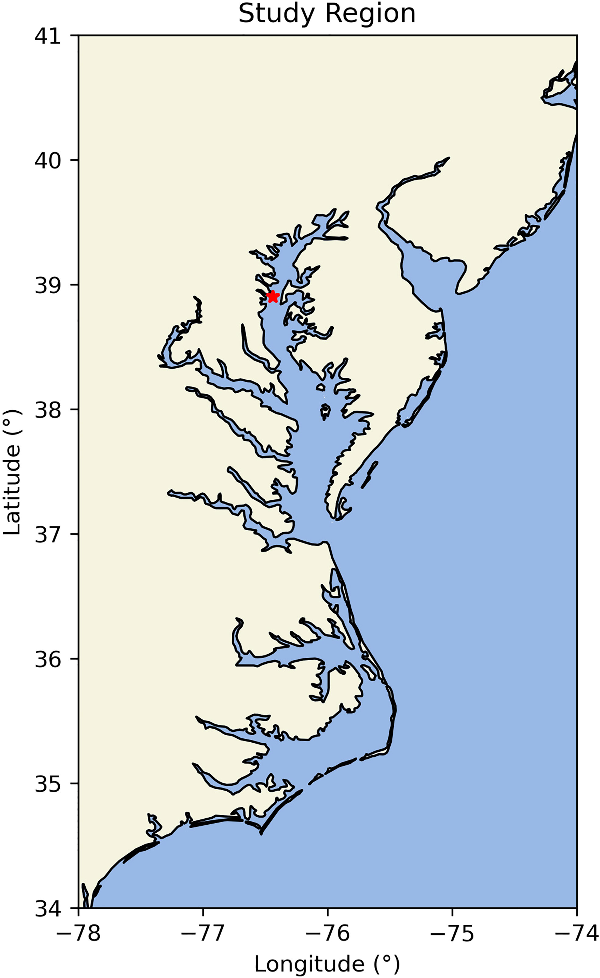
Figure 1 Location of the Thomas Point station (red star) within Chesapeake Bay.

Forecasts of near-surface air temperature were obtained from the Global Ensemble Forecast System (GEFS) model output provided as part of the Subseasonal Experiment (SubX) dataset (Pegion et al., 2019). This dataset contains a suite of retrospective forecast simulations, or reforecasts, in which a weather forecast model was initialized with historical observations and freely run forward in time to produce a forecast. The GEFS reforecasts that we used were initialized once per week (every Wednesday) from 1999 through 2016 and run for 35 days. Each reforecast simulation included 10 ensemble members, with each ensemble member beginning with slightly perturbed initial conditions and other minor differences to capture uncertainty (Zhou et al., 2017). The GEFS data were archived at 1 degree resolution, and we used an average of grid points between 38 and 40°N and -76 to -75°E to approximate air temperatures at the Thomas Point station.

To prepare the air temperature forecasts for use in forecasting water temperature, we applied a simple lead-dependent bias and drift correction. We calculated a smoothed, lead-dependent climatology for the GEFS ensemble mean using methods described in Pegion et al. (2019) and Ross et al. (2020) (except with the smoothing window reduced to ±5 days to better capture peaks) and subtracted the climatology from the GEFS reforecast to produce anomalies. The smoothed climatology calculated for the Thomas Point air temperature observations during the same time period was then added to the anomalies to produce corrected air temperature forecasts. This correction addresses mean biases and drifts in the model, including mean biases that may arise as a result of the difference in station and model air temperature height, and allows the correction to vary as a function of the forecast initialization and lead time.

Predicting SST from near-surface air temperature

Surface water temperature at the Thomas Point station was predicted from the ensemble of bias-corrected GEFS air temperature forecasts using a simple model that we adapted from models developed by Piccolroaz et al. (2013) and subsequent papers (Toffolon et al., 2014; Toffolon and Piccolroaz, 2015; Piccolroaz, 2016; Piccolroaz et al., 2016). This model predicts the time rate of change of sea surface temperature (or temperature within the surface mixed layer) as a function of the net air-sea heat flux, with the net heat flux parameterized entirely by the water and near-surface air temperatures. The model was originally developed to predict water temperature in lakes and rivers that respond rapidly to atmospheric temperature forcing. The shallow Chesapeake Bay and other coastal regions in the Northeast U.S. also respond fairly rapidly and predictably to atmospheric temperature forcing (Hare and Able, 2007; Hare et al., 2010; Muhling et al., 2018). Furthermore, the net air-sea heat flux is the primary driver of marine heatwaves in Chesapeake Bay (Mazzini and Pianca, 2022). We used an adaptation of this model because it provides both prediction skill and low computational costs.

Mathematically, the model for Chesapeake Bay SST is

$\begin{array}{ll}\frac{dW}{dt}(W,A)=\frac{H_{net}}{\rho c_{p}D}\approx \frac{{\beta }_0+{\beta }_{1}A+{\beta }_{2}W}{\delta }& (1)\end{array}$

where W and A are the surface water and air temperatures, respectively. Physically, the time rate of water surface temperature change depends on the net heat flux H_net divided by the water density ρ, the specific heat capacity c_p , and the water mixed layer depth D . The model parameterizes this rate of change using three empirically-determined β terms that relate the net heat flux to the daily mean air and water surface temperatures and a normalized depth $\delta =\frac{D}{D_0}$ which is the mixed layer depth divided by a reference mixed layer depth. Note that we have implicitly divided the β terms by ρc_pD₀ .

In Equation 1, the parameterized heat flux is distributed throughout the surface mixed layer, the depth of which must also be parameterized. We designed our parameterization to account for the seasonal variation of mixing of temperature and density in Chesapeake Bay near the Thomas Point station: temperature is typically vertically homogeneous in autumn and winter and partially stratified in spring and summer (Figure S1A) and density is usually stratified but less so in autumn and winter (Figure S1B). We parameterized the mixed layer depth using an annual harmonic:

$\begin{array}{ll}\delta =1+c_0\cos (\omega d)+s_0\sin (\omega d)& (2)\end{array}$

where ω is the angular frequency corresponding to a period of one year, d is the day of the year, and c₀ and s₀ are tunable coefficients. Consistent with expectations, in the optimized model, the mixed layer depth is highest in winter and lowest in summer (Figure S2). Adding an additional higher order harmonic did not improve the model performance. Other uses of similar SST models have parameterized the mixed layer depth using the sea surface temperature (e.g. Piccolroaz et al., 2013); however, we found that SST is not easily related to the extent of vertical mixing in Chesapeake Bay. For example, June and September have similar mean SST but different vertical temperature and density profiles (Figure S1).

To forecast future sea surface temperature from forecast future air temperature, the model in Equation 1 was initialized with water and air temperatures observed on the day before the start of the air temperature forecasts and stepped forward in time using a predictor-corrector method:

$\begin{array}{ll}\begin{array}{ll}{\widehat{W}}_{t+\text{Δ}t}=\hfill & W_t+\text{Δ}t\frac{dW}{dt}(W_t,A_t)\hfill \\ W_{t+\text{Δ}t}=\hfill & W_t+\frac{1}{2}\text{Δ}t\left(\frac{dW}{dt}(W_t,A_t)+\frac{dW}{dt}({\widehat{W}}_{t+\text{Δ}t},A_{t+\text{Δ}t})\right)\hfill \end{array}& (3)\end{array}$

where the time step Δt is one day. To prevent unphysical values and keep the simulations stable, the water temperature was restricted to values between -1°C and 40°C.

To find the optimal values of the tunable parameters in the SST model, the model was run forward in time using the time series of atmospheric temperature observed at the Thomas Point buoy during 1986 through 1998. The model ran continuously, aside from restarting with observed water temperatures during occasional interruptions in the atmospheric temperature observations. Optimization was achieved by minimizing the mean square error of the predicted water temperature compared to the observed water temperature.

After tuning on observed data from 1986 to 1998, the SST model was used to produce forecasts of SST for 1999 to 2016 using the dataset of GEFS air temperature forecasts. The GEFS dataset consists of an ensemble of 10 air temperature forecasts per initialization date, and the model in Equation 3 was run separately for each forecast to produce an ensemble of 10 SST forecasts for each date. Each forecast for a given start date was initialized with the same water and air temperature observed on the day before the initialization.

Probabilistic SST forecasts

In addition to considering the raw 10-member ensemble of SST forecasts generated for each initialization date, we applied a nonhomogeneous Gaussian regression (NGR) post-processing method to obtain probabilistic forecasts from the ensemble (Gneiting et al., 2005). NGR assumes that the probability distribution for forecast SST given a model ensemble x is a Gaussian distribution determined by the ensemble mean μ_x and the ensemble variance ${\sigma }_x^2$, shifted and scaled to adjust for biases in the mean and variance of the ensemble relative to the range of observed outcomes:

$\begin{array}{ll}P(\text{SST}\mid x)\sim \mathcal{N}(a+b{\mu }_x,c+d{\sigma }_x^2)& (4)\end{array}$

In Equation 4, a represents a mean SST forecast bias, which should be near zero in our case because the atmospheric forecasts are bias-corrected and the parameters of the SST model are optimized to minimize error. Similarly, b , which scales the ensemble mean, will ideally be near 1 for our case. The key components are the variance bias c and scaling d , which determine the variance of the probability distribution and the uncertainty of the forecast. NGR uses information about the ensemble variance to determine the forecast uncertainty. However, ensemble forecasts of the earth system are routinely underdispersive (Palmer et al., 2005), in which case the scaling term d corrects for underdispersion by inflating the variance of the ensemble and the constant term c applies a mean bias correction to the variance. For cases where the ensemble variance does not provide information about the forecast uncertainty, d = 0 and the forecast uncertainty is a constant set by c .

The four parameters in Equation 4 were determined by minimizing the continuous ranked probability score (CRPS) averaged over the complete set of retrospective forecasts, following Gneiting et al. (2005). For a single observation y and a forecast cumulative distribution function F , the CRPS is

$\begin{array}{ll}\text{CRPS(}F,y)={\displaystyle {\int }_{-\infty }^{\infty }{\left[F(t)-H(t-y)\right]}^{2}dt,}& (5)\end{array}$

where H is the Heaviside step function and t denotes a threshold. This score evaluates a probabilistic forecast of a continuous variable and is equivalent to taking the Brier score for a forecast of the probability of exceeding a threshold t and integrating it over all real thresholds (Gneiting and Raftery, 2007). If the forecast is deterministic, the CRPS is equal to the absolute error (Gneiting and Raftery, 2007). Because the forecast distribution F for nonhomogeneous Gaussian regression is a Gaussian distribution, a closed form solution for Equation 5 is

$\begin{array}{ll}\text{CRPS}\left[\mathcal{N}(\mu ,{\sigma }^2),y\right]=\sigma \left\{\frac{y-\mu }{\sigma }\left[2\text{Φ}\left(\frac{y-\mu }{\sigma }\right)-1\right]+2\phi \left(\frac{y-\mu }{\sigma }\right)-\frac{1}{\sqrt{\pi }}\right\}& (6)\end{array}$

where Φ and φ are the CDF and PDF of a normal distribution with mean 0 and variance 1 evaluated at the normalized forecast error (y−μ)/σ (Gneiting et al., 2005). An optimization algorithm was used to find the parameters a , b , c , and d that minimized the CRPS averaged over all forecasts.

Because we expected that the optimal NGR parameters will vary as the lead time changes, for example due to changing underdispersion or weakening of the relationship between ensemble variance and forecast error, a different set of parameters was derived for each forecast lead time. For a forecast lead time t , the parameters were optimized using forecasts from leads t±1 . We note that the optimization was performed using the same set of forecasts and observations that were also used to assess the skill of the probabilistic forecasts, and therefore the skill assessment could be artificially biased high. However, due to the large sample size (18 years of weekly forecasts), any artificial bias should be minimal.

We refer to the probabilistic forecasts produced using this post-processing method as calibrated forecasts because the forecast probability implied by the ensemble has been adjusted using an algorithm tuned to produce probabilities that are more consistent with the observed frequencies of events. Whether the forecast probabilities are actually consistent with the observed frequencies has also been referred to as calibration in some studies; however, we will refer to consistency between forecast probabilities and observations as reliability (Section 2.4).

To graphically demonstrate the concepts discussed in this section, Figure 2 shows the calibrated ensemble mean forecast (thick red line) derived from the 10-member SST forecast ensemble (thin red lines) for a single forecast beginning on July 26, 2006. The uncertainty in the forecast, represented by the 80% forecast interval (shaded red area), increases at later lead times. Due to the significant underdispersion of the 10-member ensemble at shorter lead times, the calibrated uncertainty in the first few days is much wider than the ensemble spread. At later lead times, as forecast skill declines, the width of the forecast interval becomes nearly constant.

FIGURE 2

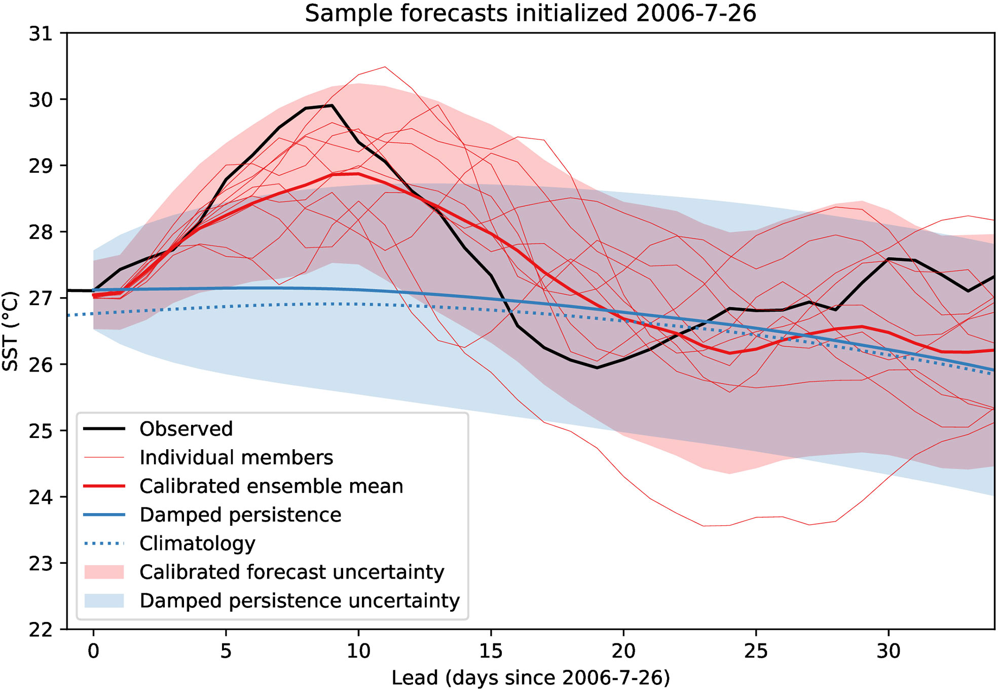
Figure 2 Demonstration of a set of model forecasts (red) and reference forecasts (blue) for SST at the Thomas Point station initialized on July 26, 2006, and the SST observed at the station (black). Shaded regions indicate 80% prediction intervals.

Evaluation of SST forecasts

The evaluation of the SST forecasts was primarily conducted using skill scores, which compare the error of the model forecasts with the error of a reference forecast such as the long-term mean value or the previously observed value (Murphy, 1988; Murphy and Epstein, 1989). A general skill score, expressed in percent, takes the form of

$\begin{array}{ll}100\%\times \frac{A(f)-A(r)}{A(p)-A(r)}& (7)\end{array}$

where A denotes an accuracy metric that compares a set of forecasts with a set of observations, f is the model forecasts, r is the set of reference forecasts, and p is a perfect forecast (for which the accuracy metric is often zero) (Murphy, 1988). A positive skill score indicates that the forecasts are more accurate than the reference forecast; the upper bound of the skill score is 100% and indicates a perfect forecast. Deterministic forecasts were primarily evaluated using the mean square error (MSE) skill score, which uses the mean square error as the accuracy metric in Equation 7. Probabilistic forecasts of SST were evaluated using the continuous ranked probability skill score (Equation 6) as the accuracy metric in Equation 7. The uncertainty of the forecast evaluation metrics was determined using the bias-corrected and accelerated bootstrap method (Efron, 1987) with 1000 samples.

The skill scores used for forecast evaluation require one or more reference forecasts for comparison. As illustrated in Figure 2, we considered two different reference forecasts in this study. First, the climatological reference forecast predicts that future SST will follow the observed climatological mean. The climatological mean SST was determined using the same smoothing method used for air temperature (Section 2.1). Because the model forecasts are bias-corrected using the climatology from 1999–2016, we used this same period to calculate the climatological forecast. Additionally, we included a linear trend term to allow the climatology to change over time, to ensure that the forecast skill does not come solely from capturing an easily predictable response to climate change. Based on the observed trend in the 1999–2016 anomalies at the Thomas Point station, the SST climatology warms at a rate of 0.37°C per decade (a trend larger than Hinson et al. (2021) found for a longer time period and broader spatial region).

The second reference forecast, the damped persistence forecast, assumes that the SST anomaly (the difference between the daily SST and the mean climatology of SST) will gradually revert from the anomaly observed prior to the initialization of the forecast to zero. We assumed that the reversion to the mean for the damped persistence forecast is consistent with a first-order autoregressive (AR1) process. The damped persistence forecast at lead time t is given by

$\begin{array}{ll}W(t)=\overline{W}(t)+{W^{\prime }}_{-1}{\varphi }^{t+1}& (8)\end{array}$

where $\overline{W}\left(t\right)$ is the climatological mean SST, W^′₋₁ is the SST anomaly observed before the start of the forecast, and ϕ is the value of the autocorrelation function at lag 1. Note that lead 0 corresponds to a 1-day-ahead forecast for the autoregressive model, hence the addition of 1 to the lead time in the exponent. The autocorrelation function was calculated using the same period of data used to calculate the climatology and using detrended anomalies (i.e. with the linear trend term used for the climatological forecast subtracted from the anomalies). Similarly, to ensure that the damped persistence forecast accounts for the long-term trend, the anomaly W^′₋₁ in Equation 8 is also the detrended anomaly, and the climatology $\overline{W}\left(t\right)$ is the 1999-2016 climatology plus the linear trend. Damped persistence can also easily be considered as a reference forecast for the evaluation of probabilistic forecasts. In this case, the probability distribution for the forecast is a Gaussian distribution with a mean given by Equation 8 and a variance given by

$\begin{array}{ll}{\sigma }_W^2(t)={\sigma }^2\frac{1-{\varphi }^{2(t+1)}}{1-{\varphi }^2}& (9)\end{array}$

where σ² is the variance of the noise in the autoregressive process.

In addition to evaluating the skill of the probabilistic forecasts using the CRPS skill score, we also assessed whether the forecasts were reliable and sharp using methods similar to those suggested by Gneiting et al. (2007). In general terms, forecast reliability refers to whether the forecast probabilities are consistent with the observed frequencies of events; for example, out of all of the times that a 10% chance of an SST threshold being exceeded was forecast, 10% of the observations should show the exceedance (Johnson and Bowler, 2009). We assessed reliability using probability integral transform (PIT) plots, which are histograms of the forecast CDF values of the actual observations. A reliable forecast model is indicated by a flat PIT plot that resembles a histogram of samples from a standard uniform distribution, while some problems such as overdispersion, underdispersion, or biases can be identified by characteristic deviations from flatness. Forecast sharpness refers to the magnitude of the range covered by the forecast probability distribution; a better, sharper forecast will have the probability concentrated within a narrower range of outcomes. We assessed forecast sharpness by comparing the median widths of the 50% and 80% prediction intervals of the forecasts as a function of lead time.

In the example forecast (Figure 2), the observed SST on the day before the first forecast day was about 0.4°C above the climatological average for that day (dotted blue line), so the damped persistence forecast (solid blue line) begins near this SST anomaly and decreases towards the long-term climatology at later lead times. Uncertainty for the damped persistence forecast (shaded blue region) is lower for the first few lead times than for the rest of the forecast due to the information provided by the previous conditions and the gradual divergence of the autoregressive process. For roughly the first two weeks of this particular forecast, the calibrated ensemble mean forecast was closer to the observed SST than the reference forecasts of climatology or damped persistence were, which indicates a skillful forecast. The calibrated 80% prediction interval was also initially sharper than the damped persistence interval. At some later lead times, the reference forecasts were more accurate, which indicates that the model forecast was not skillful at this lead time.

Extreme SST forecasts

Using the suite of retrospective, probabilistic forecasts of Chesapeake Bay SST, we also created forecasts of the probability of experiencing an extreme heat event. We considered any day in which the daily mean SST exceeds 27.5°C to be an extreme event. We note that we are considering only a single day of extreme SST to be part of an event, whereas other definitions such as multiple days of SSTs above a certain threshold or the exceedance of certain SST quantiles rather than absolute values have more commonly been considered indicators of marine heatwaves (Hobday et al., 2016; Hobday et al., 2018). We focused on a single day definition in part because estuarine SST can be more variable and less persistent than open ocean SST and also because the negative impacts of extreme SSTs can occur rapidly in estuaries and coastal regions. We primarily focused on the 27.5°C threshold because exceeding this threshold is climatologically possible (with a maximum probability of 35% in early August; Supporting Information Figure S3), which allows a large enough sample size for evaluation, but is also never more likely than not to occur. Furthermore, 27.5°C is within a range of temperatures that have negative impacts on water quality and living marine resources in the bay (Muhling et al., 2017; Shields et al., 2019). To check whether the results are sensitive to the definition of an extreme event, we also evaluated forecasts using thresholds between 26.5 and 28.5°C. We also note that under our definition of an extreme heat event as the exceedance of an absolute temperature threshold, extreme heat events can only occur during the warm season. Mazzini and Pianca (2022) found that heatwaves defined using the traditional Hobday et al. (2016) definition, which can occur during any time of the year, occurred most frequently in the summer in Chesapeake Bay.

Evaluation of extreme SST forecasts

To assess the potential value of extreme SST forecasts, we applied an approach developed by Richardson (2000) and Wilks (2001) and recently applied by Kiaer et al. (2021). This method evaluates forecasts of an event occurrence based on the real or hypothetical value of using the forecasts to make a decision to avoid harmful impacts and financial losses associated with the event occurring. The evaluation takes place in a binary context where forecasts are used to decide whether or not to take action to protect against a potential event, and subsequently the event and its impacts either do or do not occur (summarized in Table 1). For example, exceeding the 27.5°C heatwave threshold could be considered an event; the loss associated with this event could be healthcare costs to treat infection with pathogenic Vibrio bacteria that grow rapidly at warmer temperatures (Ralston et al., 2011; Davis et al., 2017; Collier et al., 2021); and the action taken to avoid these impacts could be a temporary suspension of fishing and recreation if temperatures above 27.5°C are forecast.

TABLE 1

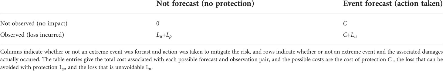
Table 1 Framework for evaluation of forecast value.

For an individual event-forecast pair, no cost is incurred for a correct forecast of no event. If an event is forecast and protective action is taken but the event does not occur, the cost of protection (C; for example, loss of fishing and recreational income) is incurred. If an event and the need for protection is correctly forecast to occur, the cost is C plus any unavoidable loss L_u associated with the event that occurs regardless of protection. Finally, if an event is not forecast but it does occur, both L_u and the loss that could have been prevented with protection, L_p , are incurred. To use this framework to evaluate the forecasts, the costs associated with the observed outcomes and the hypothetical forecast-driven decisions are added up over time and compared with the costs that would have been incurred using a reference or perfect forecast instead, following the framework for general skill scores (Equation 7).

It can be shown that the unavoidable loss L_u cancels out during calculation of the value skill score (Wilks, 2001), and the resulting score depends only on the forecasts, observations, and the ratio of the cost of protection to the preventable loss C/L_p . Probabilistic forecasts can be converted into binary decisions using this same ratio; if the forecast probability of a harmful event is less than C/L_p , no protective action should be taken because the expected loss is less than the cost of protection, but if the forecast probability is greater than C/L_p , protective action is expected to be beneficial and should be taken (Wilks, 2001). We used this rule to convert the probabilistic SST model forecasts and the reference forecasts of damped persistence and climatology (discussed next) into binary decisions. We also evaluated a deterministic forecast of the ensemble mean SST forecast; in this case, protective action is always taken when the ensemble mean exceeds the 27.5°C event threshold. We evaluated the forecasts over a range of values of C/L_p greater than 0 but less than 1; note that action is free and always taken when C/L_p=0 , and action is expensive and never taken when C/L_p>1 .

To calculate the climatological reference forecast needed for the skill score, (1) for each calendar day of year, we determined the fraction of days that exceeded the SST threshold during 1999–2016 (the empirical probability), and (2) we used the same smoothing method applied in Section 2.1 obtain a smooth climatology of the heat wave probability as a function of the day of year (Supporting Information Figure S3). In this case, we did not include a trend term in the climatology because it would be difficult to accurately estimate a trend in rare events over such a short time period.

Results

SST model

When run as a nearly continuous hindcast using the air temperature observed at the Thomas Point station, the model can accurately predict SST (Table 2). A modest negative bias (i.e., the model predictions are cooler than the observations) develops during the testing period, which could reflect the warming trend induced by climate change. Despite the worsened bias, the RMSE, MAE, and skill score are similar during the training and testing periods. This bias also should not affect the forecast simulations, which only run for 35 days after being initialized with observed SST. The parameters of the optimized SST model are provided in Table 3.

TABLE 2

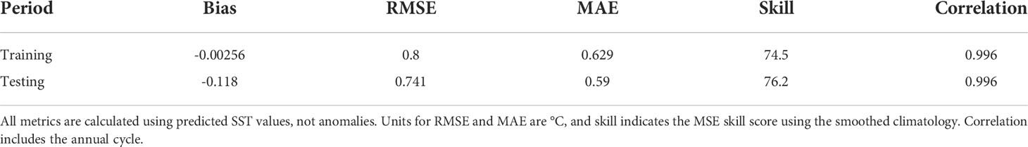
Table 2 Skill of the SST model hindcast during the training (1986–1998) and testing (1999–2016) periods.

TABLE 3

Table 3 Optimized values of the parameters in the model for SST (Equation 1).

Air and SST forecast evaluation

Compared to observations at the Thomas Point station, the ensemble mean of the GEFS retrospective forecasts for daily mean air temperature exhibits significant skill for about two weeks after forecast initialization. The first five forecast days have a root mean square error below 2°C (Figure 3A). The surface air temperature forecast errors contain a weak periodicity as a result of the weekly forecast initializations; for example, a large error associated with an extreme event that occurred at lead 6 in one set of forecasts will also occur at leads 13, 20, or 27 in forecasts initialized in prior weeks. Air temperature forecast error increases fairly linearly during the first two weeks, and overall the forecast skill scores are significantly greater than zero through lead 12 (Figure 3B). RMSE for leads 0-3 is lower for damped persistence than for climatology, resulting in lower skill scores when using damped persistence as the reference metric. Beyond lead 3, the damped persistence and climatology scores are essentially the same. This rapid convergence is consistent with the weak autocorrelation of the atmosphere, which results in a damped persistence forecast that quickly reverts from the initial condition to the long-term climatology. When separated by season (Figure 3C), the air temperature forecast skill relative to damped persistence reaches zero fastest for the summer, while the skill is generally highest for the winter.

FIGURE 3

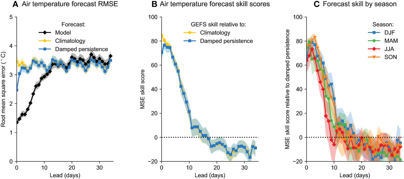
Figure 3 (A) Root mean square error of all GEFS ensemble mean air temperature forecasts compared with the error of the climatology and damped persistence reference forecasts. (B) Mean square error skill scores for all ensemble mean air temperature forecasts relative to the climatology and damped persistence reference forecasts. (C) MSE skill scores calculated separately for each season, using only damped persistence as the reference forecast. In all panels, shaded regions are 90% confidence intervals.

The calibrated forecasts of sea surface temperature remain significantly skillful for up to 17 days of lead time, much longer than the forecasts of air temperature (Figure 4). SST forecast errors are substantially lower than air temperature forecast errors (Figure 4A). These lower errors are consistent with the stronger autocorrelation and weaker variance of SST anomalies compared to air temperature anomalies. However, this stronger autocorrelation and weaker variance also results in lower skill scores for SST forecasts (Figure 4B), even though the skill scores remain positive for longer. Like air temperature, damped persistence is the most challenging reference forecast to beat (the lowest error and skill scores). SST forecasts generally follow the air temperature pattern of higher skill for longer lead times in the winter than in the summer (Figures 4C, D). Despite the use of this idealized model, the skill of the spring, summer, and fall forecasts is closely comparable to the skill found in numerical model simulations for the same time period by Ross et al. (2020).

FIGURE 4

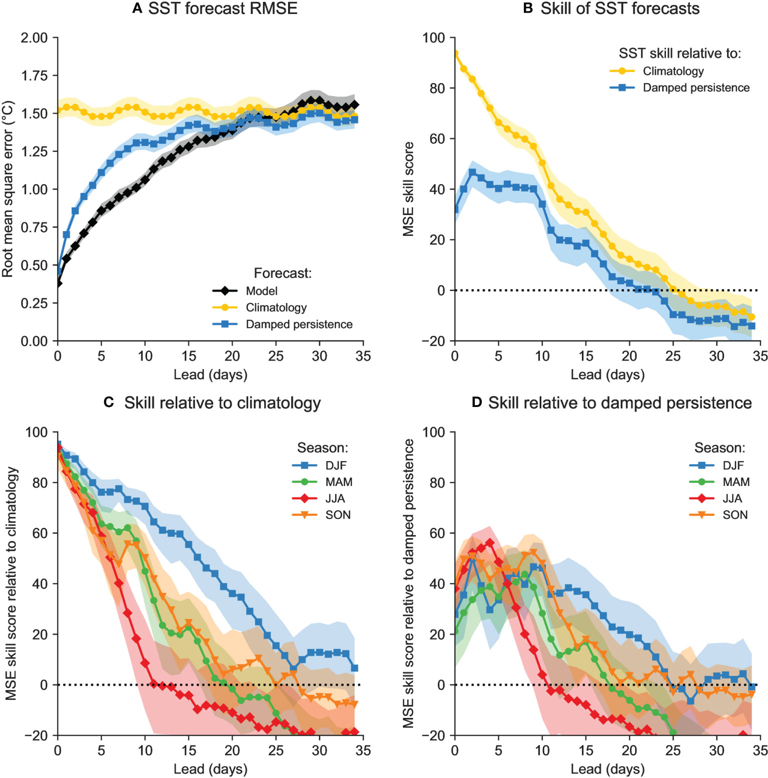
Figure 4 (A) Mean square error skill scores for calibrated SST forecasts over all forecast times. (B) MSE skill scores for each season, for the climatology reference forecast. (C, D) MSE skill scores for each season, using climatology (C) and damped persistence (D) as the reference forecasts. In all panels, shaded regions are 90% confidence intervals.

Figure 5A shows the values of the four parameters used in the NGR forecast calibration (Equation 4). The parameters a and b are near 0 and 1, respectively, indicating that mean biases in the SST forecasts are negligible. The parameter d is above one for the first week (aside from the first two days), indicating that the variance of the ensemble must be inflated to reliably capture the forecast uncertainty. However, because the ensemble variance is small in the early part of the forecast, the inflated ensemble variance dσ² nevertheless remains small relative to the total calibrated forecast variance (Figure 5B). The small value of the ensemble-informed variance dσ² relative to the fixed variance correction c suggests that the ensemble spread has a weak correlation with the forecast uncertainty and that the primary effect of the NGR post-processing is to give each forecast the same variance c .

FIGURE 5

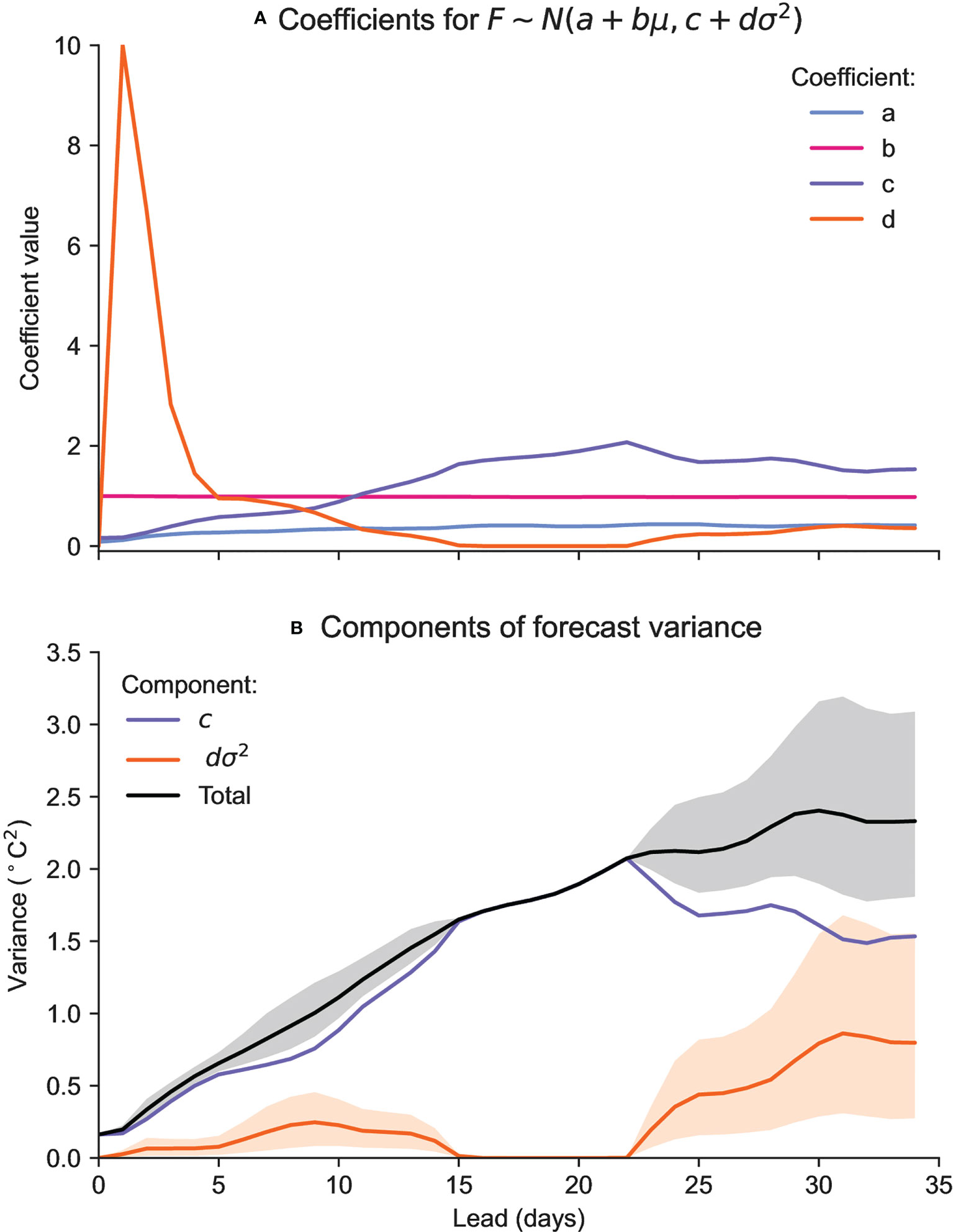
Figure 5 (A) NGR parameters used to calibrate the probabilistic forecasts. (B) Contribution of the variance bias correction c and the ensemble spread dσ² to the total variance of the calibrated probabilistic forecasts. Solid lines are averages over all forecasts, and shaded regions denote 10-90% percentiles.

In the evaluation of the probabilistic forecasts, the forecasts calibrated using NGR are skillful compared to the reference forecast of damped persistence (Figures 6A, B). To test whether the post-processing improved the forecast skill, we also calculated the CRPS score for the raw model ensemble using the empirical CDF of the ensemble (Hersbach, 2000) and compared with the score for the calibrated model. Using a probabilistic forecast derived directly from the variance of the raw model ensemble results in significantly lower CRPS skill due to the underdispersive nature of the raw ensemble. Skill for the calibrated forecasts remains significantly positive out to 17 days of lead time, matching the skill of the deterministic forecasts (Figure 4). However, the CRPS skill score is much lower than the MSE skill score at earlier lead times (before about 10 days), suggesting that there is room for improvement in the representation of forecast uncertainty at early leads. When separated by season, the skill is highest in the winter and lowest in the spring and summer, again consistent with the skill of the deterministic forecasts.

FIGURE 6

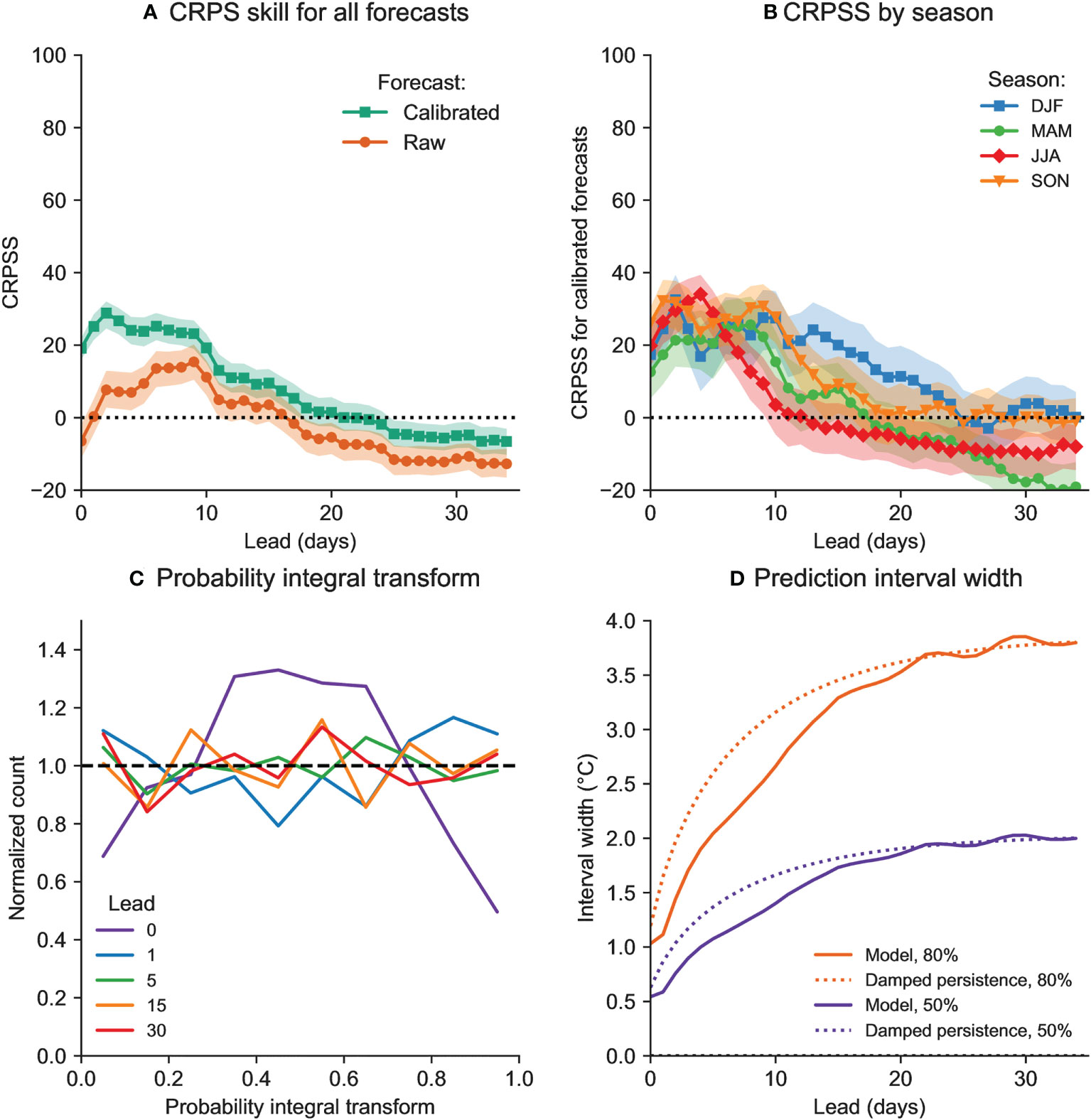
Figure 6 Assessment of the probabilistic forecasts. (A) Skill metrics based on the continuous ranked probability score (CRPS) for all forecasts. This figure compares the NGR calibrated forecasts (Section 2.3) with probabilistic forecasts where the uncertainty is determined by the raw ensemble. (B) Skill scores for the calibrated forecasts evaluated separately by initialization season. In both panels (A) and (B), shaded regions are 90% confidence intervals. (C) Probability integral transform plots for various forecast lead times. (D) Median widths of the 50 and 80 percent prediction intervals for the calibrated and damped persistence forecasts.

The NGR post-processing generally produced reliable probabilistic forecasts (Figure 6C). Representation of uncertainty appears to be challenging in the first few days of the forecast: the post-processed lead-0 forecasts are overdispersive (observations falling disproportionately in the middle of the forecast distribution) and the lead-1 forecasts are slightly underdispersive (observations disproportionately in the tails of the forecast distribution). By 5 days of lead time, however, the forecasts appear to be reliable, as indicated by nearly flat lines. In addition to being reliable, the forecasts are also reasonably sharp (Figure 6D). The model forecasts have substantially narrower prediction intervals than the damped persistence reference forecast during early leads. At lead times beyond about 20 days, the interval widths for both forecasts converge and plateau, consistent with unskillful forecasts of the climatological probability distribution.

Forecasting extreme SSTs

The simple model for forecasting Chesapeake Bay sea surface temperature examined in the previous section showed skill at producing both deterministic and probabilistic forecasts of SST. In this section, we evaluate whether the SST forecasts can be applied to predict and avoid the impacts of extreme SSTs.

The extreme forecasts show significant value when applied in the idealized decision-making framework detailed in Section 2.6. For lead 5 (Figure 7A), making decisions using the calibrated probabilistic forecast would result in substantial value beyond the benefit of using the climatological probability of experiencing an extreme SST for nearly all values of the cost to preventable loss ratio (with statistical significance for ratios below 0.5). The calibrated probabilistic model forecasts also generally have higher value than the probability given by the damped persistence forecast, suggesting that the modest skill of the probabilistic forecasts (Figure 6) nevertheless may provide meaningful and actionable information to decision-makers.

FIGURE 7

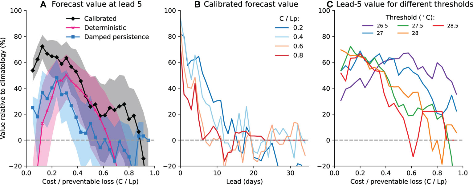
Figure 7 Relative value of heatwave forecasts. (A) The relative value of calibrated probabilistic forecasts, the deterministic forecasts using the ensemble mean, and the probabilistic damped persistence reference forecasts at 5 days lead time. Shaded regions are 90% confidence intervals. (B) Relative value of the calibrated probabilistic forecasts at all lead times. (C) Relative value of the calibrated forecasts using different thresholds of an extreme event ranging from 26.5 to 28.5°C. Confidence intervals are not shown in (B) or (C) for clarity.

Using the deterministic forecast, which entails ignoring all information about probability and simply taking protective action when the ensemble mean SST forecast is above the extreme threshold, also results in value for moderate values of the cost-loss ratio. Note that this method of using the deterministic forecast is essentially equivalent to deciding to protect whenever the forecast probability is above 50%; as a result, the value of the deterministic forecast resembles the value of the calibrated forecast when C/L_p is near 0.5, and the value is less than the calibrated forecasts for low values of C/L_p (when the deterministic forecast too rarely results in protection) and for high values of C/L_p (when the deterministic forecast too frequently results in protection).

The value of the calibrated probabilistic forecast is generally higher, and the calibrated forecasts are generally valuable for longer lead times, when C/L_p is smaller (Figure 7B). This pattern partially reflects the quickly increasing uncertainty in the SST forecasts—the high forecast probability required to take action when C/L_p is high rarely or never occurs in long-lead forecasts, and in this case the forecasts result in the same lack of action as the climatological reference case for high C/L_p . Note that in Figure 7A, the damped persistence reference forecast similarly has no value for high values of C/L_p at lead 5. In contrast, strong persistence of initial anomalies means that initial or early warm SSTs can correctly cause a small increase in the forecast extreme temperature probability, which, when C/L_p is small, can sometimes result in the correct decision to take action. It is also important to note that the value score is generally expected to be maximized at a C/L_p ratio equal to the observed frequency of the event being forecast (Richardson, 2000). As a result, it is expected that forecast value will be higher at low values of C/L_p when forecasting extreme events. However, in this study, the observed frequency varies seasonally, so the relation between the observed frequency and the C/L_p ratio with maximum value may not strictly hold.

The value of the forecasts depends similarly on the threshold used to define an extreme event (Figure 7C). Although the values for thresholds between 27 and 28.5°C generally have similar relationships to C/L_p , the value for the 26.5°C threshold shows an opposite pattern of lower value for low C/L_p and higher value for moderate to high C/L_p . Following the same reasoning as before, it is expected that the region of highest value will shift towards higher C/L_p as the temperature threshold is lowered and the climatological probability and observed frequency of exceeding the threshold increases.

Discussion

Sources of forecast errors and possible improvements to the model system

Our analysis of SST forecast skill in the Chesapeake Bay applied a simple model that predicts SST as a function of only the previously observed SST, the forecast air temperature, and the time of year. This simple model greatly reduced the computational requirements of this study and enabled the rapid generation of the large number of ensemble simulations necessary to generate and evaluate the probabilistic forecasts. The model also produced SST forecasts with skill roughly comparable to the forecasts produced with a dynamical ocean model (Ross et al., 2020). However, the idealized model neglects drivers of SST variability other than those that can be directly related to air and water temperature and time of year, which could reduce the forecast skill, and is also incapable of predicting other ecologically relevant variables such as bottom temperature. The idealized model thus provided an important framework for testing forecast methods and potential forecast skill, but expansion of this approach to an ensemble of dynamical model forecasts will be an essential future step.

A limitation of the simple model applied in this study is that it predicts daily mean sea surface temperature and does not resolve sub-daily temperature variability. At the study site, the difference between the daily mean SST and the daily maximum SST averages as low as 0.4°C in the winter to as high as 0.9°C in the summer (Supporting Information Figure S4). The variability of the maximum-mean difference is also higher in the summer. For applications that are especially sensitive to the exceedance of a specific threshold for a short period of time, this mean variability could be accounted for by reducing the daily mean temperature threshold accordingly, or the simple model could be modified to predict daily high or low temperatures and explicitly include the effects of downwelling shortwave radiation and other forcing predicted by the atmospheric model.

The model also does not account for wind-driven anomalies in SST. Wind events in the summer can increase mixing and reduce stratification (Scully, 2010; Xie and Li, 2018), resulting in lower SSTs as cooler deep water is mixed to the surface. Depending on direction, winds can also drive lateral circulation (Li and Li, 2011; Li and Li, 2012) and cause upwelling or downwelling and estuary-shelf exchange at the mouth of the bay (Paraso and Valle-Levinson, 1996). However, the latter two effects are likely small at the central upper-bay location analyzed in this study. To test whether wind-driven mixing could contribute to SST forecast errors, in Figure 8A, we compare the errors of SST forecasts with 5 days of lead time with the mean wind speed for all forecasts initialized between June and August. These results do show that increased wind speed results in positive SST forecast errors (observations cooler than forecast), although the overall contribution to the forecast error is small (R²=0.08 ).

FIGURE 8

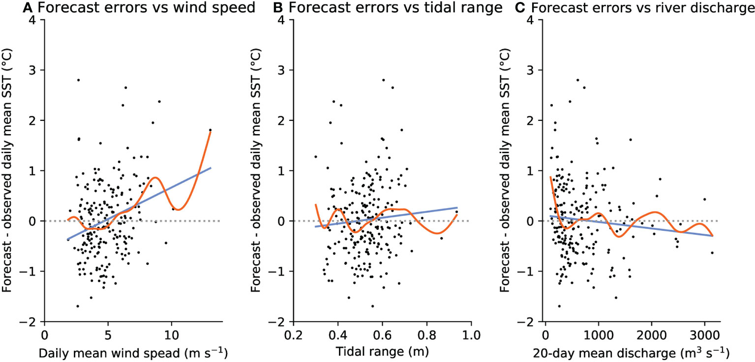
Figure 8 Errors of all 5 day lead summer forecasts compared with (A) the mean wind speed on the forecast verification day, (B) the tidal range on the forecast verification day, and (C) the discharge from the Susquehanna River averaged over the 20 days before the forecast verification day. In all subfigures, the solid orange line shows a generalized additive model fit to the data, and the solid blue line shows a linear fit to the data.

SST forecast errors could also be caused by variations in tidally driven mixing (such as the spring-neap cycle) which are not explicitly included in the simple model. In Figure 8B, we compare summer SST errors with tidal range. Tidal range was computed by taking hourly water levels from the NOAA tide gauge at Tolchester Beach, MD and calculating the difference between the daily maximum and daily minimum water level. Variations in tidal range appears to have a negligible effect on the SST forecast error (R²=0.006 ).

Finally, SST forecast errors could also be caused by river discharge to the bay. Processes throughout the Chesapeake Bay are strongly driven by river discharge (e.g. Jiang and Xia, 2016; Jiang and Xia, 2017), and about half of the total freshwater entering the bay is discharged by the Susquehanna River (Schubel and Pritchard, 1986). Increased river discharge increases salinity stratification in the bay, potentially resulting in a shallower mixed layer than predicted by the seasonal cycle of depth in the forecast model and producing errors in the forecast SST change. High river discharge also contributes a large volume of river water that may have a different temperature than the ambient bay water. In Figure 8C, we compare the summer SST forecast errors with discharge from the Susquehanna River measured at the Conowingo Dam averaged over the 20 days before the forecast verification date. Variations in river discharge also appear to have a negligible effect on the SST forecast error (R²=0.009 ). Two factors could help explain this negligible effect. First, river discharge has a strong seasonal cycle, and by including a seasonal cycle of mixed layer depth in the SST forecast model (Equation 2), we are able to capture the primary influence of river discharge on mixed layer depth and SST. Second, our analysis of temperature extremes and forecast errors has focused on summer, and Susquehanna River discharge is typically lowest in summer and autumn.

Potential improvements to forecast pre- and post-processing

Before using the air temperature forecasts as input to the SST model, the drifts and biases in the forecasts were removed by subtracting a smoothed climatology that was a function of the lead time and initialization day of year. This correction only adjusts the mean of the air temperature forecasts and does not remove other potential problems such as an incorrect climatological variance or a wrong distribution. We assessed the distributions of the observed and forecast air temperature anomalies and found that both were well-represented by nearly identical normal distributions (Figure S5). The similarity of the distributions suggests that a mean bias correction is sufficient, and we assumed that any of the minor errors in variance seen in Figure S5 would be corrected by the NGR post-processing step if they affected the SST forecasts. If the forecasts were not as well-behaved, bias correction methods that correct the full distribution of the model data [e.g., Cannon et al. (2015)] could be applied. One challenge of using these methods for correcting forecasts is that accurately estimating a correction to apply to the full distribution requires a substantially longer retrospective forecast period than merely estimating the mean.

During the forecast post-processing, forecast uncertainty was represented with a Gaussian distribution determined by the ensemble mean and variance. However, distributions with heavier tails, such as the logistic or t distributions, could give better prediction of extreme events and account for additional forecast uncertainty introduced by the estimation of the post-processing parameters (Siegert et al., 2016; Gebetsberger et al., 2018). Similarly, the minimum negative log-likelihood (or maximum likelihood), rather than the minimum CRPS, is an alternative calibration target that places heavier penalties on events in the tails of the forecast distribution (Gebetsberger et al., 2018). We tested post-processing the forecasts with logistic distributions fitted by minimizing the negative log-likelihood and found that it did not improve the value of the probabilistic forecasts (not shown). This result is consistent with the probability integral transform plot (Figure 6) which shows that the forecasts based on Gaussian distributions are generally reliable.

The four parameters used in the NGR post-processing method were assumed to depend only on the forecast lead time and were fit using all of the available retrospective forecast and observation data for a given lead. However, these parameters could be allowed to vary over time to capture changes or seasonal variability in the properties of the SST model forecasts. In short-term weather forecasts, a rolling window of forecasts and observations from the most recent days or weeks is often used to train the post-processing algorithm (e.g. Stensrud and Skindlov, 1996). This window allows the post-processing method to handle complications such as seasonal variations in model bias or spread or changes in weather regimes that affect predictability. Alternatively, the post-processing parameters could be fit separately for each calendar month or season to capture regular seasonal variability in model properties. Although in this study we only allowed the post-processing parameters to vary with lead time, future studies should experiment with other forms of time dependence for the parameters.

Potential applications of extreme SST and marine heatwave forecasts

The weather-scale extreme SST forecasts developed in this study have potential applications to managing fisheries and water quality issues that can arise quickly during high temperature excursions. In some cases, weather forecasts of air temperature have already been applied in an attempt to address these issues. For example, the Maryland Department of Natural Resources has recently issued advisories that recommend striped bass fishers take precautions when air temperature is forecast to exceed 90°F (about 32°C) and discourage striped bass fishing after 10 a.m. when air temperature is forecast to exceed 95°F (35°C) (Chesapeake Bay Magazine, 2019). These voluntary advisories are intended to reduce the mortality that occurs when striped bass are caught and released at times when the air and water is unusually warm. Similar and more robust advisories could be issued with the SST forecasts developed in this study, and the value-based assessment framework could be used to evaluate whether using forecasts to make decisions improves the tradeoff between the cost of reducing fishing when a heatwave is forecast and the loss of fish from catch-and-release mortality.

Current methods to reduce the risk of Vibrio bacteria in oysters rely on restricting harvest times and requiring rapid cooling of harvested oysters during months when the average water temperature exceeds a certain threshold (Froelich and Noble, 2016). This management method is essentially the same as the climatological reference forecast used in the value-based assessment framework—protective action is always taken when a certain climatological probability of dangerously warm water is exceeded. After a careful forecast skill assessment, with an appropriate emphasis on the need to protect public health, forecasts of air and water temperatures could be applied to determine when stricter harvest controls are beneficial and necessary or when looser controls could be permitted. In particular, forecasts may be useful for managing and adapting to climate change by identifying times when protective action needs to be taken outside of the time period when it was historically necessary.

In addition to reducing the ecosystem and public health impacts of extreme events, forecasts could also be used to reduce the economic impacts on fishers by enabling them to adjust their harvest to compensate for expected closures or decreases in catch. For example, Jin and Hoagland (2008) note that fishers may use short-term harmful algal bloom forecasts to increase their harvest before a bloom occurs and the fishery is closed. However, similar applications of forecasts, such as temperature-based forecasts of the timing of lobster landings in the Gulf of Maine, have had unanticipated effects and raised ethical concerns (Pershing et al., 2018; Hobday et al., 2019). Fortunately, reliable probabilistic forecasts with robustly assessed skill, such as those developed in the present study, can help reduce the potential for unintended consequences and avoid ethical issues (Hobday et al., 2019).

Conclusion

Our study presented a set of methods for developing and evaluating probabilistic forecasts of SST and extreme SST events in an estuary. These forecasts showed significant skill and have valuable potential to inform decisions to protect against damages associated with extreme events. In the idealized decision-making framework, accounting for uncertainty by using the calibrated probabilistic forecasts lead to better decisions than simply considering the deterministic ensemble mean forecast for most values of the ratio of the cost of taking protective action to the preventable loss. These forecasts were skillful despite the simple nature of the SST model, which predicted SST solely from forecasts of atmospheric temperature. Future studies should consider improvements to the SST model and conduct more detailed evaluations of applications that could benefit from probabilistic SST forecasts.

Data availability statement

The raw data supporting the conclusions of this article will be made available by the authors, without undue reservation.

Author contributions

AR conducted the analysis and wrote the first draft of the manuscript. CS provided guidance and contributed suggestions and edits on several revisions of the manuscript. Both authors read and approved the submitted version.

Funding

This report was partially prepared under award NA18OAR4320123 from the National Oceanic and Atmospheric Administration, U.S. Department of Commerce and with funding from the Climate Program Office (grant “Seasonal to interannual ocean habitat forecasts for the Northeast U.S. Large Marine Ecosystem”) and the Integrated Ecosystem Assessment program.

Acknowledgments

The authors acknowledge Hyung-Gyu Lim and Nathaniel Johnson for their comments and suggestions on an internal review of this manuscript, and Keith Dixon and Kathy Pegion for discussions that improved the manuscript.

Conflict of interest

The authors declare that the research was conducted in the absence of any commercial or financial relationships that could be construed as a potential conflict of interest.

The reviewer AH declared a past co-authorship with the author CS to the handling editor.

Publisher’s note

All claims expressed in this article are solely those of the authors and do not necessarily represent those of their affiliated organizations, or those of the publisher, the editors and the reviewers. Any product that may be evaluated in this article, or claim that may be made by its manufacturer, is not guaranteed or endorsed by the publisher.

Author disclaimer

The statements, findings, conclusions, and recommendations are those of the authors and do not necessarily reflect the views of the National Oceanic and Atmospheric Administration, or the U.S. Department of Commerce.

Supplementary material

The Supplementary Material for this article can be found online at: https://www.frontiersin.org/articles/10.3389/fmars.2022.896961/full#supplementary-material

References

Baker-Austin C., Trinanes J., Gonzalez-Escalona N., Martinez-Urtaza J. (2017). Non-cholera vibrios: The microbial barometer of climate change. Trends Microbiol. 25, 76–84. doi: 10.1016/j.tim.2016.09.008

PubMed Abstract | CrossRef Full Text | Google Scholar

Cannon A. J., Sobie S. R., Murdock T. Q. (2015). Bias correction of GCM precipitation by quantile mapping: How well do methods preserve changes in quantiles and extremes? J. Climate 28, 6938–6959. doi: 10.1175/JCLI-D-14-00754.1

CrossRef Full Text | Google Scholar

Chesapeake Bay Magazine (2019) Wild Chesapeake: New striped bass advisories help save catch & release fish. Available at: https://chesapeakebaymagazine.com/wild-chesapeake-new-striped-bass-advisories-help-save-catch-release-fish/.

Google Scholar

Collier S. A., Deng L., Adam E. A., Benedict K. M., Beshearse E. M., Blackstock A. J., et al. (2021). Estimate of burden and direct healthcare cost of infectious waterborne disease in the United States. Emerging Infect. Dis. 27, 140–149. doi: 10.3201/eid2701.190676

CrossRef Full Text | Google Scholar

Davis B. J. K., Jacobs J. M., Davis M. F., Schwab K. J., DePaola A., Curriero F. C. (2017). Environmental determinants of Vibrio parahaemolyticus in the Chesapeake Bay. Appl. Environ. Microbiol. 83, AEM.01147–17. doi: 10.1128/AEM.01147-17

CrossRef Full Text | Google Scholar

Efron B. (1987). Better bootstrap confidence intervals. J. Am. Stat. Assoc. 82, 171–185. doi: 10.2307/2289144

CrossRef Full Text | Google Scholar

Froelich B. A., Noble R. T. (2016). Vibrio bacteria in raw oysters: Managing risks to human health. philosophical transactions of the royal society of London. Ser. B Biol. Sci., 371. doi: 10.1098/rstb.2015.0209

CrossRef Full Text | Google Scholar

Frölicher T. L., Fischer E. M., Gruber N. (2018). Marine heatwaves under global warming. Nature 560, 360–364. doi: 10.1038/s41586-018-0383-9

PubMed Abstract | CrossRef Full Text | Google Scholar

Gale M. K., Hinch S. G., Donaldson M. R. (2013). The role of temperature in the capture and release of fish. Fish Fisheries 14, 1–33. doi: 10.1111/j.1467-2979.2011.00441.x

CrossRef Full Text | Google Scholar

Gebetsberger M., Messner J. W., Mayr G. J., Zeileis A. (2018). Estimation methods for nonhomogeneous regression models: Minimum continuous ranked probability score versus maximum likelihood. Monthly Weather Rev. 146, 4323–4338. doi: 10.1175/MWR-D-17-0364.1

CrossRef Full Text | Google Scholar

Gneiting T., Balabdaoui F., Raftery A. E. (2007). Probabilistic forecasts, calibration and sharpness. J. R. Stat. Society: Ser. B (Statistical Methodology) 69, 243–2168. doi: 10.1111/j.1467-9868.2007.00587.x

CrossRef Full Text | Google Scholar

Gneiting T., Raftery A. E. (2007). Strictly proper scoring rules, prediction, and estimation. J. Am. Stat. Assoc. 102, 359–378. doi: 10.1198/016214506000001437

CrossRef Full Text | Google Scholar

Gneiting T., Raftery A. E., Westveld A. H., Goldman T. (2005). Calibrated probabilistic forecasting using ensemble model output statistics and minimum CRPS estimation. Monthly Weather Rev. 133, 1098–1118. doi: 10.1175/MWR2904.1

CrossRef Full Text | Google Scholar

Green T. J., Siboni N., King W. L., Labbate M., Seymour J. R., Raftos D. (2019). Simulated marine heat wave alters abundance and structure of vibrio populations associated with the Pacific oyster resulting in a mass mortality event. Microbial Ecol. 77, 736–747. doi: 10.1007/s00248-018-1242-9

CrossRef Full Text | Google Scholar

Groner M. L., Hoenig J. M., Pradel R., Choquet R., Vogelbein W. K., Gauthier D. T., et al. (2018). Dermal mycobacteriosis and warming sea surface temperatures are associated with elevated mortality of striped bass in Chesapeake Bay. Ecol. Evol. 8, 9384–9397. doi: 10.1002/ece3.4462

PubMed Abstract | CrossRef Full Text | Google Scholar

Hare J. A., Able K. W. (2007). Mechanistic links between climate and fisheries along the East Coast of the United States: Explaining population outbursts of Atlantic croaker (Micropogonias undulatus). Fisheries Oceanography 16, 31–45. doi: 10.1111/j.1365-2419.2006.00407.x

CrossRef Full Text | Google Scholar

Hare J. A., Alexander M. A., Fogarty M. J., Williams E. H., Scott J. D. (2010). Forecasting the dynamics of a coastal fishery species using a coupled climate–population model. Ecol. Appl. 20, 452–464. doi: 10.1890/08-1863.1

PubMed Abstract | CrossRef Full Text | Google Scholar

Hersbach H. (2000). Decomposition of the continuous ranked probability score for ensemble prediction systems. Weather Forecasting 15, 559–570. doi: 10.1175/1520-0434(2000)015<0559:DOTCRP>2.0.CO;2

CrossRef Full Text | Google Scholar

Hinson K. E., Friedrichs M. A., St-Laurent P., Da F., Najjar R. G. (2021). Extent and causes of Chesapeake Bay warming. JAWRA J. Am. Water Resour. Assoc. 1–21. doi: 10.1111/1752-1688.12916

CrossRef Full Text | Google Scholar

Hobday A. J., Alexander L. V., Perkins S. E., Smale D. A., Straub S. C., Oliver E. C., et al. (2016). A hierarchical approach to defining marine heatwaves. Prog. Oceanography 141, 227–238. doi: 10.1016/j.pocean.2015.12.014

CrossRef Full Text | Google Scholar

Hobday A. J., Hartog J. R., Manderson J. P., Mills K. E., Oliver M. J., Pershing A. J., et al. (2019). Ethical considerations and unanticipated consequences associated with ecological forecasting for marine resources. ICES J. Mar. Sci. 76:1244-56. doi: 10.1093/icesjms/fsy210

CrossRef Full Text | Google Scholar

Hobday A., Oliver E., Sen Gupta A., Benthuysen J., Burrows M., Donat M., et al. (2018). Categorizing and naming marine heatwaves. Oceanography 31, 162–173. doi: 10.5670/oceanog.2018.205

CrossRef Full Text | Google Scholar

Jacox M. G., Alexander M. A., Siedlecki S., Chen K., Kwon Y.-O., Brodie S., et al. (2020). Seasonal-to-interannual prediction of North American coastal marine ecosystems: Forecast methods, mechanisms of predictability, and priority developments. Prog. Oceanography 183, 102307. doi: 10.1016/j.pocean.2020.102307

CrossRef Full Text | Google Scholar

Jacox M. G., Tommasi D., Alexander M. A., Hervieux G., Stock C. A. (2019). Predicting the evolution of the 2014–2016 California current system marine heatwave from an ensemble of coupled global climate forecasts. Front. Mar. Sci. 6. doi: 10.3389/fmars.2019.00497

CrossRef Full Text | Google Scholar

Jiang L., Xia M. (2016). Dynamics of the Chesapeake Bay outflow plume: Realistic plume simulation and its seasonal and interannual variability. J. Geophysical Research: Oceans 121, 1424–1445. doi: 10.1002/2015JC011191

CrossRef Full Text | Google Scholar

Jiang L., Xia M. (2017). Wind effects on the spring phytoplankton dynamics in the middle reach of the Chesapeake Bay. Ecol. Model. 363, 68–80. doi: 10.1016/j.ecolmodel.2017.08.026

CrossRef Full Text | Google Scholar

Jin D., Hoagland P. (2008). The value of harmful algal bloom predictions to the nearshore commercial shellfish fishery in the Gulf of Maine. Harmful Algae 7, 772–781. doi: 10.1016/j.hal.2008.03.002

CrossRef Full Text | Google Scholar

Jöhnk K. D., Huisman J., Sharples J., Sommeijer B., Visser P. M., Stroom J. M. (2008). Summer heatwaves promote blooms of harmful cyanobacteria. Global Change Biol. 14, 495–512. doi: 10.1111/j.1365-2486.2007.01510.x

CrossRef Full Text | Google Scholar

Johnson C., Bowler N. (2009). On the reliability and calibration of ensemble forecasts. Monthly Weather Rev. 137, 1717–1720. doi: 10.1175/2009MWR2715.1

CrossRef Full Text | Google Scholar

Kiaer C., Neuenfeldt S., Payne M. R. (2021). A framework for assessing the skill and value of operational recruitment forecasts. ICES J. Mar. Sci. 78, 3581–3591. doi: 10.1093/icesjms/fsab202

CrossRef Full Text | Google Scholar

Laufkötter C., Zscheischler J., Frölicher T. L. (2020). High-impact marine heatwaves attributable to human-induced global warming. Science. 369,:1621–1625. doi: 10.1126/science.aba0690

PubMed Abstract | CrossRef Full Text | Google Scholar

Li Y., Li M. (2011). Effects of winds on stratification and circulation in a partially mixed estuary. J. Geophysical Res. 116. doi: 10.1029/2010JC006893

CrossRef Full Text | Google Scholar

Li Y., Li M. (2012). Wind-driven lateral circulation in a stratified estuary and its effects on the along-channel flow. J. Geophysical Research: Oceans 117. doi: 10.1029/2011JC007829

CrossRef Full Text | Google Scholar

Lindegren M., Brander K. (2018). Adapting fisheries and their management to climate change: A review of concepts, tools, frameworks, and current progress toward implementation. Rev. Fisheries Sci. Aquaculture 26, 400–415. doi: 10.1080/23308249.2018.1445980

CrossRef Full Text | Google Scholar

Liu G., Eakin C. M., Chen M., Kumar A., de la Cour J. L., Heron S. F., et al. (2018). Predicting heat stress to inform reef management: NOAA Coral Reef Watch's 4-month coral bleaching outlook. Front. Mar. Sci. 5. doi: 10.3389/fmars.2018.00057

CrossRef Full Text | Google Scholar

Mazzini P. L. F., Pianca C. (2022). Marine heatwaves in the Chesapeake Bay. Front. Mar. Sci. 8. doi: 10.3389/fmars.2021.750265

PubMed Abstract | CrossRef Full Text | Google Scholar

Muhling B. A., Gaitán C. F., Stock C. A., Saba V. S., Tommasi D., Dixon K. W. (2018). Potential salinity and temperature futures for the Chesapeake Bay using a statistical downscaling spatial disaggregation framework. Estuaries Coasts 41, 349–372. doi: 10.1007/s12237-017-0280-8

CrossRef Full Text | Google Scholar

Muhling B. A., Jacobs J., Stock C. A., Gaitán C. F., Saba V. S. (2017). Projections of the future occurrence, distribution, and seasonality of three vibrio species in the Chesapeake Bay under a high-emission climate change scenario. GeoHealth 124, 419–489. doi: 10.1002/2017GH000089

CrossRef Full Text | Google Scholar

Murphy A. H. (1988). Skill scores based on the mean square error and their relationships to the correlation coefficient. Monthly Weather Rev. 116, 2417–2424. doi: 10.1175/1520-0493(1988)116<2417:SSBOTM>2.0.CO;2

CrossRef Full Text | Google Scholar

Murphy A. H. (1991). Probabilities, odds, and forecasts of rare events. Weather Forecasting 6, 302–07. doi: 10.1175/1520-0434(1991)006<0302:POAFOR>2.0.CO;2

CrossRef Full Text | Google Scholar

Murphy A. H., Epstein E. S. (1989). Skill scores and correlation coefficients in model verification. Monthly Weather Rev. 117, 572–582. doi: 10.1175/1520-0493(1989)117<0572:SSACCI>2.0.CO;2

CrossRef Full Text | Google Scholar

Oliver E. C. J., Burrows M. T., Donat M. G., Sen Gupta A., Alexander L. V., Perkins-Kirkpatrick S. E., et al. (2019). Projected marine heatwaves in the 21st century and the potential for ecological impact. Front. Mar. Sci. 6. doi: 10.3389/fmars.2019.00734

CrossRef Full Text | Google Scholar

Paerl H. W., Huisman J. (2008). Blooms like it hot. Science 320, 57–58. doi: 10.1126/science.1155398

PubMed Abstract | CrossRef Full Text | Google Scholar

Palmer T., Shutts G., Hagedorn R., Doblas-Reyes F., Jung T., Leutbecher M. (2005). Representing model uncertainty in weather and climate prediction. Annu. Rev. Earth Planetary Sci. 33, 163–193. doi: 10.1146/annurev.earth.33.092203.122552

CrossRef Full Text | Google Scholar

Paraso M. C., Valle-Levinson A. (1996). Meteorological influences on sea level and water temperature in the lower Chesapeake Bay: 1992. Estuaries 19, 548–561. doi: 10.2307/1352517

CrossRef Full Text | Google Scholar

Pegion K., Kirtman B. P., Becker E., Collins D. C., LaJoie E., Burgman R., et al. (2019). The subseasonal experiment (SubX): A multi-model subseasonal prediction experiment. Bull. Am. Meteorological Soc. 100, 2043–2060. doi: 10.1175/BAMS-D-18-0270.1

CrossRef Full Text | Google Scholar

Pershing A., Mills K., Dayton A., Franklin B., Kennedy B. (2018). Evidence for adaptation from the 2016 marine heatwave in the Northwest Atlantic ocean. Oceanography 31,:152–161. doi: 10.5670/oceanog.2018.213

CrossRef Full Text | Google Scholar

Piccolroaz S. (2016). Prediction of lake surface temperature using the air2water model: Guidelines, challenges, and future perspectives. Adv. Oceanography Limnology 7, 36–50. doi: 10.4081/aiol.2016.5791

CrossRef Full Text | Google Scholar

Piccolroaz S., Calamita E., Majone B., Gallice A., Siviglia A., Toffolon M. (2016). Prediction of river water temperature: A comparison between a new family of hybrid models and statistical approaches. Hydrological Processes 30, 3901–3917. doi: 10.1002/hyp.10913

CrossRef Full Text | Google Scholar

Piccolroaz S., Toffolon M., Majone B. (2013). A simple lumped model to convert air temperature into surface water temperature in lakes. Hydrology Earth System Sci. 17, 3323–38. doi: 10.5194/hess-17-3323-2013

CrossRef Full Text | Google Scholar

Ralston E. P., Kite-Powell H., Beet A. (2011). An estimate of the cost of acute health effects from food- and water-borne marine pathogens and toxins in the USA. J. Water Health 9, 680–694. doi: 10.2166/wh.2011.157

PubMed Abstract | CrossRef Full Text | Google Scholar

Ramos M. H., Van Andel S. J., Pappenberger F. (2013). Do probabilistic forecasts lead to better decisions? Hydrology Earth System Sci. 17, 2219–2232. doi: 10.5194/hess-17-2219-2013

CrossRef Full Text | Google Scholar

Richardson D. S. (2000). Skill and relative economic value of the ECMWF ensemble prediction system. Q. J. R. Meteorological Soc. 126, 649–667. doi: 10.1002/qj.49712656313

CrossRef Full Text | Google Scholar

Ross A. C., Stock C. A., Dixon K. W., Friedrichs M. A. M., Hood R. R., Li M., et al. (2020). Estuarine forecasts at daily weather to subseasonal time scales. Earth Space Sci. 7. doi: 10.1029/2020EA001179

CrossRef Full Text | Google Scholar

Roulston M. S., Bolton G. E., Kleit A. N., Sears-Collins A. L. (2006). A laboratory study of the benefits of including uncertainty information in weather forecasts. Weather Forecasting 21, 116–122. doi: 10.1175/WAF887.1

CrossRef Full Text | Google Scholar

Sanford E., Sones J. L., García-Reyes M., Goddard J. H. R., Largier J. L. (2019). Widespread shifts in the coastal biota of northern California during the 2014–2016 marine heatwaves. Sci. Rep. 94216. doi: 10.1038/s41598-019-40784-3

PubMed Abstract | CrossRef Full Text | Google Scholar

Schubel J. R., Pritchard D. W. (1986). Responses of upper Chesapeake Bay to variations in discharge of the Susquehanna River. Estuaries 9, 236–249. doi: 10.2307/1352096

CrossRef Full Text | Google Scholar

Scully M. E. (2010). Wind modulation of dissolved oxygen in Chesapeake Bay. Estuaries Coasts 33, 1164–1175. doi: 10.1007/s12237-010-9319-9

CrossRef Full Text | Google Scholar

Shields E. C., Parrish D., Moore K. (2019). Short-term temperature stress results in seagrass community shift in a temperate estuary. Estuaries Coasts 42, 755–764. doi: 10.1007/s12237-019-00517-1

CrossRef Full Text | Google Scholar

Siegert S., Sansom P. G., Williams R. M. (2016). Parameter uncertainty in forecast recalibration. Q. J. R. Meteorological Soc. 142, 1213–1221. doi: 10.1002/qj.2716

CrossRef Full Text | Google Scholar

Smith G., Spillman C. (2019). New high-resolution sea surface temperature forecasts for coral reef management on the Great Barrier Reef. Coral Reefs 38, 1039–1056. doi: 10.1007/s00338-019-01829-1

CrossRef Full Text | Google Scholar

Stensrud D. J., Skindlov J. A. (1996). Gridpoint predictions of high temperature from a mesoscale model. Weather Forecasting 11, 103–110. doi: 10.1175/1520-0434(1996)011<0103:GPOHTF>2.0.CO;2

CrossRef Full Text | Google Scholar

Stock C. A., Pegion K., Vecchi G. A., Alexander M. A., Tommasi D., Bond N. A., et al. (2015). Seasonal sea surface temperature anomaly prediction for coastal ecosystems. Prog. Oceanography 137, 219–236. doi: 10.1016/j.pocean.2015.06.007

CrossRef Full Text | Google Scholar

Toffolon M., Piccolroaz S. (2015). A hybrid model for river water temperature as a function of air temperature and discharge. Environ. Res. Lett. 10, 114011. doi: 10.1088/1748-9326/10/11/114011

CrossRef Full Text | Google Scholar

Toffolon M., Piccolroaz S., Majone B., Soja A.-M., Peeters F., Schmid M., et al. (2014). Prediction of surface temperature in lakes with different morphology using air temperature. Limnology Oceanography 59, 2185–2202. doi: 10.4319/lo.2014.59.6.2185

CrossRef Full Text | Google Scholar

Tommasi D., Stock C. A., Pegion K., Vecchi G. A., Methot R. D., Alexander M. A., et al. (2017). Improved management of small pelagic fisheries through seasonal climate prediction. Ecol. Appl. 27, 378–388. doi: 10.1002/eap.1458

PubMed Abstract | CrossRef Full Text | Google Scholar

Wilks D. S. (2001). A skill score based on economic value for probability forecasts. Meteorological Appl. 8, 209–219. doi: 10.1017/S1350482701002092

CrossRef Full Text | Google Scholar

Xie X., Li M. (2018). Effects of wind straining on estuarine stratification: A combined observational and modeling study. J. Geophysical Research: Oceans 123, 2363–2380. doi: 10.1002/2017JC013470

CrossRef Full Text | Google Scholar

Zhou X., Zhu Y., Hou D., Luo Y., Peng J., Wobus R. (2017). Performance of the new NCEP global ensemble forecast system in a parallel experiment. Weather Forecasting 32, 1989–2004. doi: 10.1175/WAF-D-17-0023.1

CrossRef Full Text | Google Scholar