 Christina A. Frieder1
 Chao Yan2
 Marcelo Chamecki2Daniel Dauhajre2James C. McWilliams2
 Javier Infante3
 Meredith L. McPherson4
 Raphael M. Kudela4
 Fayçal Kessouri5
 Martha Sutula5Isabella B. Arzeno-Soltero1
 Kristen A. Davis1,6*
- 1Department of Civil and Environmental Engineering, University of California, Irvine, Irvine, CA, United States
- 2Department of Atmospheric and Oceanic Sciences, University of California, Los Angeles, Los Angeles, CA, United States
- 3Patagonia Seaweeds, Puerto Varas, Chile
- 4Department of Ocean Sciences, University of California, Santa Cruz, Santa Cruz, CA, United States
- 5Southern California Coastal Water Research Project, Costa Mesa, CA, United States
- 6Department of Earth System Science, University of California, Irvine, Irvine, CA, United States
Offshore aquaculture has the potential to expand the macroalgal industry. However, moving into deeper waters requires suspended structures that will present novel farm-environment interactions. Here, we present a computational modeling framework, the Macroalgal Cultivation Modeling System (MACMODS), to explore within-farm modifications to light, seawater flow, and nutrient fields across time and space scales relevant to macroalgae. A regional ocean model informs the site-specific setting, the Santa Barbara Channel in the Southern California Bight. A fine-scale hydrodynamic model predicts modified flows and turbulent mixing within the farm. A spatially resolved macroalgal growth model, parameterized for giant kelp, Macrocystis pyrifera, predicts kelp biomass. Key findings from model integration are that regional ocean conditions set overall farm performance, while fine-scale within-farm circulation and nutrient delivery are important to resolve variation in within-farm macroalgal performance. Therefore, we conclude that models resolving within-farm dynamics can provide benefit to farmers with insight on how farm design and regional ocean conditions interact to influence overall yield. Here, the presence of repeating longlines aligned with the mean current generate flow diversions around the farm as well as attached Langmuir circulations and increased turbulence intensity. These flow-induced phenomena lead to less biomass in the interior portion of the farm relative to the edges. We also find that there is an effluent “footprint” that extends as much as 20 km beyond the farm. In this regard, MACMODS can be used to not only evaluate farm design and cultivation practices that maximize yield but also explore interactions between the farm and ecosystem in order to minimize impacts.
1. Introduction
At the global scale, marine macroalgae, or seaweed, are primarily cultivated in nearshore waters as food products (FAO, 2018), but there is recent interest in expanding seaweed farming offshore. Offshore macroalgal farming has the potential to contribute to energy security and reduce greenhouse gas emissions through biofuel production and to provide low-emission alternatives for industries as diverse as textiles, bioplastics, and fertilizers. Large-scale cultivation of seaweeds and sinking of biomass is also being evaluated as a strategy for ocean-based carbon sequestration (Froehlich et al., 2019; Hoegh-Guldberg et al., 2019). While there is potential to build a thriving marine biomass industry (Duarte et al., 2017), mass-cultivation is in its nascency and there are barriers to development (Fernand et al., 2017; Campbell et al., 2019). Numerical modeling can be a useful tool for optimizing farm designs, cultivation techniques, and operational procedures to maximize yield, for siting farms, and for predicting impacts and benefits to coastal ecosystems.
Farming offshore in deeper water requires suspended cultivation systems that present novel and complex hydrodynamics that can determine nutrient availability within the farm and thus farm performance (Figure 1, Yan et al., 2021). Seaweed imposes a hydrodynamic drag on the flow that reduces mean velocity and increases seawater residence time in natural kelp beds and in farm settings (Thom, 1971; Jackson, 1997; Gaylord et al., 2007; Delaux et al., 2011). Flow reduction within the farm can lead to the development of shear layers at the bottom of the canopy (Plew, 2011), which produce coherent eddies with potential to increase entrainment of deeper nutrient-rich water. However, current understanding of flow dynamics within suspended farms is mostly limited to models with simple flow conditions (Delaux et al., 2011; Zhou and Venayagamoorthy, 2019), laboratory flume experiments utilizing rigid cylinders (Plew, 2011), and sparse field observations from mussel aquaculture (Plew et al., 2005, 2006). Detailed numerical studies show that flow modifications induced by the farm interact with waves and turbulence in non-trivial ways (Yan et al., 2021). In particular, farm designs with organized longlines can lead to the development of secondary flow structures that strongly impact nutrient availability within the farm (Yan et al., 2021).
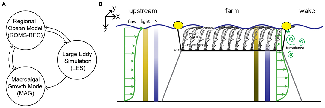
Figure 1. (A) Relation among models used in this study. Solid lines represent flow of information in full-farm simulations. Dotted line represents additional pathway not included in current study. (B) Conceptual diagram illustrating the longline farm design for cultivation of Macrocystis pyrifera and anticipated farm-environment modifications. Coordinate system indicated. The along-farm perspective depicts a single longline with macroalgae cultivated at a depth of zcult. The presence of a suspended macroalgal farm modifies flow (both seawater velocity and turbulence), light, and nutrient conditions within and in the wake of the farm relative to upstream conditions. Longlines are aligned parallel to the x-dimension and repeated at a fixed distance (not shown; y-dimension). Macroalgae are cultivated along growth lines that extend in the y-dimension from the longline at a constant zcult.
Resolving within-farm flow and nutrient delivery will be fundamental to predict macroalgal productivity (Roleda and Hurd, 2019). Nutrient uptake kinetics are dependent on external nutrient concentrations and can be maximized with sufficient seawater flow and waves that act to thin diffusive boundary layers (Hurd, 2017). However, there are scenarios in which thinning of diffusive boundary layers has no impact on overall growth when seawater nutrient supply is insufficient (Hepburn et al., 2007). For seaweed cultivation systems, in general, macroaglae perform better at locations with a combination of optimal flow and maximal nutrient supply. For example, line cultivation of Undaria pinnatifida in Spain yielded higher biomass at relatively exposed vs. sheltered sites (Peteiro and Freire, 2011). While in the heavily farmed Sanggou Bay, China, kelp farming is concentrated at the mouth of the bay where nutrient delivery is sufficient relative to within the bay (Shi et al., 2011; Zhang et al., 2016; Wang et al., 2018).
The objective of the present paper is to model the 3-dimensional environment that a 16-hectare anchored seaweed farm occupies (Figure 1). We present an integration of multiple models that span time and space scales relevant to the farm. Upstream physical and chemical conditions are informed by a regional ocean model with biogeochemical elemental cycling (ROMS-BEC). A fine-scale hydrodynamic model (large-eddy simulation; LES) predicts modified hydrodynamics within the farm. A macroalgal growth model predicts kelp biomass and utilizes input from both ROMS-BEC and LES. We assess the effect of processes such as kelp shading, kelp drag, kelp nutrient drawdown, and modified nutrient transport on kelp growth. The regional ocean model is further utilized to explore modified circulation on the shelf in the presence of a suspended farm. Simulations are parameterized for giant kelp, Macrocystis pyrifera, to evaluate offshore farm potential in the Southern California Bight.
Below we provide a description of each model, detail how the models are integrated with each other (Figure 1A), and provide the setup for the four full-farm simulations performed. These full-farm simulations are an expansion on Yan et al. (2021) in which LES was utilized to evaluate modifications to within-farm hydrodynamics with a similar farm setup. Yan et al. (2021) demonstrated that the farm design consisting of a series of longlines spaced horizontally in the crossflow direction leads to the development of persistent secondary circulations that increase the exchanges between water flowing through the farm and underneath it. We demonstrate how these findings impact within farm nutrient fields, kelp nutrient uptake rates, and seasonal and spatial patterns in kelp performance. We also present results of the modification of shelf circulation in the presence of a farm when farm drag is included in ROMS-BEC.
2. Methods
2.1. Regional Ocean Conditions
We utilize an eddy-resolving oceanic physical-biogeochemical model (ROMS-BEC) of the California Current System to generate average daily physical and biogeochemical conditions from 2000–2005 (Deutsch et al., 2021; Renault et al., 2021). ROMS simulates the ocean currents by solving the hydrostatic, primitive equations (Shchepetkin and McWilliams, 2005) in a terrain-following coordinate system and uses a K-Profile Parameterization (KPP) for vertical mixing (Large et al., 1994). These ocean currents partially control the coupled biogeochemical variability simulated online with BEC (described in Deutsch et al., 2021). BEC simulates distinct nutrient cycles (nitrogen, silicic acid, phosphate, and iron), organic matter, dissolved oxygen, and carbonate chemistry.
The ROMS-BEC simulations comprise a family of one-way nested solutions that successively increase resolution and decrease spatial extent (Mason et al., 2010). For the present analysis, the horizontal resolution is 1 km with 60 vertical levels, nested down from a 4-km parent solution (see Kessouri et al., 2020; Renault et al., 2021). This solution contains tidal forcing and synoptically variable atmospheric forcing prescribed by a 6-km resolution Weather Research and Forecast Model (WRF, Skamarock et al., 2008). Relevant ROMS-BEC parameters utilized by the macroalgal growth model include nitrate, ammonium, dissolved organic nitrogen, temperature, photosynthetically active radiation (PAR), concentration of chlorophyll-a (for light attenuation due to phytoplankton shading), and seawater velocities. Wave characteristics for the corresponding historical time period were downloaded from observational buoy data available from the National Data Buoy Center (NDBC; Station 46053).
The ROMS-BEC inputs to the macroalgal growth model exhibit both seasonal and higher-frequency variability (Figure 2), indicative of the complex flows and inherent nonlinearity of the coupled biogeochemistry. The ROMS-BEC simulation has a horizontal resolution of 1 km that fully resolves mesoscale variability and partially captures submesoscale variability (McWilliams, 2016); both regimes will impact on biogeochemistry (Kessouri et al., 2020). Specific to the shelf, higher resolution (e.g., on the order of 100 m) simulations produce small-scale flow patterns in the nearshore that can impact material fluxes and thus biogeochemistry (Dauhajre et al., 2019), however, computational costs (time and storage) limit production of multi-year, higher resolution simulations. Despite these computational constraints, we expect the 1-km simulation to adequately capture the seasonality of the inputs to the macroalgal growth model.
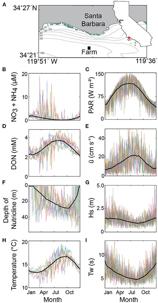
Figure 2. (A) The simulated farm (black square) is located off Santa Barbara (red star in California inset) in 60-m water depth. Presence of kelp canopy from 2000–2005 along the Santa Barbara coastline as measured from Landsat satellite sensors indicated in green (data obtained from Santa Barbara Coastal LTER). (B–I) Synopsis of environmental input conditions to the macroalgal growth model predicted by the eddy-resolving oceanic physical-biogeochemical model (ROMS-BEC). Data plotted to illustrate seasonal trends and the high-frequency variability of these in time. Individual colored lines are single years (2000–2005) and plotted as daily averages within farming depths (surface to zcult). Black thick lines are the daily mean across all years and smoothed. DON is dissolved organic nitrogen. Nutricline depth is the minimum depth at which NO3+NH4 is greater than 1 μM. PAR is the incoming photosynthetically active radiation just below the sea surface. is the magnitude horizontal seawater velocity on the farm grid. Hs is the significant wave height. Tw is the average wave period.
2.2. Fine-Scale Hydrodynamic Model
High-resolution Large-Eddy Simulations (LES) are used to study flow within and around the macroalgal farm, capturing motions in the range of scales between one and 100 m. In LES, most of the unsteady three-dimensional turbulent eddies are explicitly resolved on the numerical grid, and only the small-scale eddies that are more universal need to be parameterized (Pope, 2000). Because it requires fewer assumptions about the flow, this approach is particularly well suited for studying complex flows in which the main features are not well understood. LES has been used in studies of ocean turbulence since the mid 1990's (Skyllingstad and Denbo, 1995; McWilliams et al., 1997). We adopt the usual approach of solving the wave-averaged Navier-Stokes equations, in which surface wave motions are not explicitly resolved but their impact in the flow is represented via Stokes drift, together with the Boussinesq approximation. The LES approach and model setup employed here are described in detail in Yan et al. (2021), and only a brief description is provided below. For more details on the application of LES to ocean flow, please refer to the review paper by Chamecki et al. (2019).
The set of equations used in this study consists of the continuity equation (conservation of mass) under the Boussinesq approximation
the wave-averaged Navier-Stokes equations
and the advection-diffusion equation for seawater density fluctuations (caused by temperature fluctuations)
In this system of equations, seawater density ρ, Eulerian velocity u = (u, v, w), and generalized pressure Π are evolved on the three-dimensional numerical grid represented using cartesian coordinates x = (x, y, z), with z being the vertical direction and ez the vertical unit vector. In addition, ρ0 is the reference density, f is the Coriolis frequency, g is the gravitational acceleration, and us and ug represent the Stokes drift velocity and the mean current in geostrophic balance, respectively. The effect of the small scales (i.e., the subgrid scales; SGS) on the resolved scales is represented by the SGS momentum flux tensor τ and the buoyancy flux vector τρ. Molecular viscosity is neglected on the basis of the high-Reynolds number flows considered here.
The terms on the right-hand side of Equation (2) are the pressure-gradient force (I), the Coriolis force (II), the forces resulting from the wave-averaging procedure (III), the buoyant force from the Boussinesq approximation (IV), the drag force exerted by the macroalgal farm (V), and the SGS force (VI). The pressure-gradient force is split into a fluctuating component (−∇Π) and a mean component that is used to drive the mean flow (fez × ug, where ug is an imposed geostrophic velocity that in practice determines the strength and direction of the mean pressure-gradient force). The first of the two terms including the Stokes drift is the vortex force with being the vorticity vector (Craik and Leibovich, 1976), which is key to driving Langmuir turbulence in the upper ocean (Leibovich, 1983), and the second term represents the interaction between Stokes drift and Coriolis. For simplicity, we only consider steady monochromatic waves, so that the Stokes drift velocity is given by
In Equation (4), is the Stokes drift velocity at the surface, k is the wavenumber, ew is a unit vector in the direction of the wave propagation, and aw and ω are the wave amplitude and angular frequency.
Solution of Equations (1)–(3) require closure models for the SGS terms and the drag force exerted by the farm. The SGS momentum flux is parameterized using the scale-dependent dynamic Smagorinsky model (Bou-Zeid et al., 2005), and the SGS density flux is parameterized using a gradient-diffusion model with diffusivity obtained from the SGS viscosity and a constant Schimdt number Sc = 0.4 (Yang et al., 2015). Finally, as the numerical grid is too coarse to resolve the geometry of the macroalgae fronds and stipes, we represent their effect on the flow through a body force that represents the total drag within a grid cell given by,
Here, CD = 0.0148 is the drag coefficient according to the field experiments by Utter and Denny (1996), a is the total frond surface area per unit volume of space (obtained by conversion of the algal biomass; Supplementary Table 1), and the projection coefficient tensor P acts to yield the effective surface area facing each direction (in the present case we use P = (1/2)I, where I is the 3 × 3 identity matrix). The motion of macroalgae elements in response to the flow can be estimated based on their geometry, modulus of elasticity and buoyancy (Luhar and Nepf, 2011; Henderson, 2019). As a first approximation, we assume that the macroalgae move with the wave orbital wave velocity and thus pose no impact on the wave field (Yan et al., 2021).
Thus, in the modeling approach adopted here, the ocean state experienced by the farm is mostly determined by the surface fluxes (wind stress u∗ and surface buoyancy flux B0), the mean current (ug), the Stokes drift profile (imposed by specifying wave parameters k, aw, and ω), and the stratification in the pycnocline (represented by a constant temperature gradient). These forcings evolve continuously on diurnal and seasonal time scales, producing a wide range of ocean conditions. LES is not suitable to produce a continuous year-long simulation of evolving ocean conditions due to computational limitations. In the present work, we adopt a simplified approach in which we use LES to study a few “typical” conditions with steady forcing (i.e., no temporal changes in the ocean state) and then use ROMS-BEC results to modulate the flow features uncovered in these few LES runs (see below for more details).
We consider two cases with different surface forcing leading to distinct upper mixed-layer depths: (1) a deep, upper-boundary-layer case characteristic of winter and (2) a shallower, upper-boundary-layer case typical of summer. In both cases, we simulate neutral boundary layers with no incoming or outgoing buoyancy flux at the surface (i.e., B0 = 0). Fluid below the mixed layer is stably stratified with a constant initial potential temperature gradient dθ/dz = 0.01 °C m−1. In the deep boundary layer case, the wind stress at the surface is , corresponding to a wind speed at 10-m height above the surface of . The surface wave has a wavelength of λ = 60 m (k = 2π/λ) and a wave amplitude of aw = 0.8 m. The resulting Stokes drift at the surface is , yielding a turbulent Langmuir number that is representative of equilibrium wind-wave conditions in the open ocean (Belcher et al., 2012). This results in a boundary-layer depth zi ≈ 25 m. For the shallow, upper-boundary-layer case, we reduce the surface forcing to and , resulting in a shallower upper boundary layer with zi ≈ 15 m. In both cases, a steady current is also imposed to represent the effect of ocean currents or mesoscale eddies (assuming that mesoscale spatial and temporal variability is negligible in the LES domain). This current speed occurs through the year, but is more characteristic of the summer (Figure 2E). For the sake of simplicity, we assume that the wind, the waves, and the mean current are all aligned in the same direction. More details about the numerical model and the simulation setup can be found in Yan et al. (2021), and the geometry of the farm used in the LES runs is described in Section 2.4.
2.3. Macroalgal Growth Model
The macroalgal growth model (MAG) is developed for Macrocystis pyrifera. Existing macroalgal growth models informed the conceptual framework of the model presented here (Jackson, 1987; Solidoro et al., 1997; Broch and Slagstad, 2012; Hadley et al., 2015). We have compared our model selection to alternative forms of the growth model and found that our calculations of biomass are robust to model selection (Appendix A). Nitrogen is tracked in six pools between seawater and macroalgae: nitrate (NO3), ammonium (NH4), dissolved organic nitrogen (DON), particulate organic nitrogen (PON), stored nitrogen in macroalgae (Ns), and fixed nitrogen in macroalgae (Nf) (Figure 3A). The currency of nitrogen has been selected as this is the nutrient limiting productivity for M. pyrifera along the U.S. West Coast (Zimmerman and Kremer, 1984, 1986). For conversion to carbon units, M. pyrifera has an average C:N ratio of 16.6, but this value varies greatly in natural kelp, between 6 and 48, given macroalgae's ability to store intracellular pools of both carbon and nitrogen (Rassweiler et al., 2018). Partitioning between pools of internal nitrogen (Ns and Nf) is a two-step uptake process where nitrogen is first stored in intracellular pools and then assimilated into the macroalgae's cellular structure and is adapted from Hadley et al. (2015). There is a minimum amount of nitrogen required, Qmin (mg N g-dry-1), and the nutrient quota, Q, defines the relative nitrogen status of macroalgae.
Novel aspects of the MAG model developed here are the accounting of individual fronds, the inclusion of demographic rates of fronds such as initiation, age, growth, and senescence, and the upward growth of macroalgae through the water column. Holdfasts and sporophylls are not included in the model as they contribute little to uptake and growth (Gerard, 1982; Arnold and Manley, 1985). Fronds are categorized as subsurface, water-column, and canopy (following Rassweiler et al., 2018, depicted in Figure 1). “Subsurface” fronds are those that have not reached the surface. Fronds that have reached the surface are treated in two sections: the “water-column” section is the portion of frond that is underwater stretching from the cultivation depth to the sea surface and the “canopy” section is the portion of the frond that floats at the sea surface. Conversion between frond nitrogen and other allometric parameters is based on relationships that have been established for M. pyrifera (Supplementary Table 1). The conversion between nitrogen content and biomass is calculated as:
Biological parameters used by MAG are provided in Table 1. New fronds are initiated, Si, as a function of the average nutrient quota, Q, of existing fronds given that light at depth is greater than the compensating light irradiance. New fronds are initiated with Ns,i and Nf,i that is equivalent to 1-m frond with an average Q of existing fronds. Frond senescence is age dependent with a maximum life span of Agemax (Rodriguez et al., 2013).
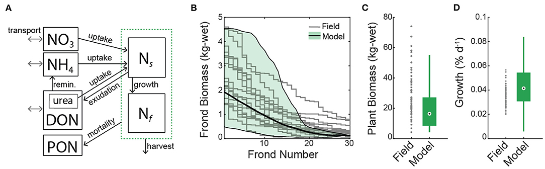
Figure 3. (A) Conceptual diagram of the macroalgal growth model. Nitrogen is partitioned between seawater and macroalgae (green dashed box). Transformation pathways among state variables are indicated (black lines with arrowhead). Dissolved nutrients undergo transport (gray lines with arrowheads). Ns, stored nitrogen in macroalgae; Nf, fixed nitrogen in macroalgae; DON, dissolved organic nitrogen in seawater; PON, particulate organic nitrogen in seawater. (B–D) Comparison of the macroalgal growth model with field surveys of Macrocystis pyrifera conducted by the Santa Barbara Coastal Long Term Ecological Research Program at Mohawk Reef. (B) Field measurement of the distribution of biomass (kg-wet) among fronds from a single plant [gray lines; n=17 plants; Reed and Rassweiler (2018)] compared with daily frond biomass predicted by the model (solid black line is the average and full range in shaded green). (C) Total plant biomass from surveyed plants compared with the model. (D) Field-derived growth rates compared with daily growth rates from the model [Equation (20)]. Box plots are median, upper and lower quartiles, and maximum and minimum values.
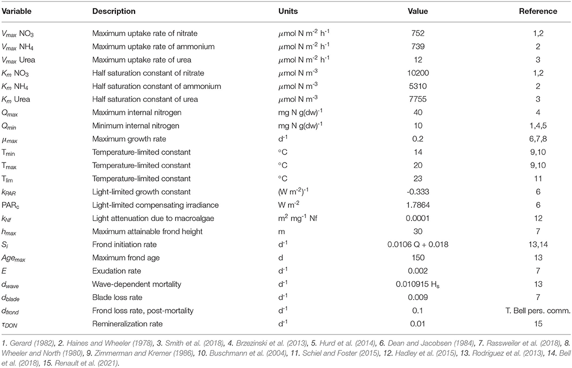
Table 1. Biological parameters for the macroalgal growth model.
Macroalgal growth is modeled as a two-step process. Nitrogen is taken up from seawater into an internal reserve of stored nitrogen (Ns; mg N m-3). Ns is converted into fixed nitrogen via growth (Nf; mg N m-3). The change in Ns over time is a result of uptake of nitrogen from seawater (U; mg N g-dry-1 d-1), growth (G; d-1), exudation (E; d-1), mortality (M; d-1), harvest (H), and frond initiation [Si; Equation (8)].
Since M. pyrifera is buoyant, fronds extend upward. Ns is vertically resolved along the length of the frond at a resolution of dz = 1 m. Translocation of Ns is a physiological phenomenon in which Ns is redistributed through a network of sieve tubes on the scale of multiple meters per day (Parker, 1965; Schmitz and Lobban, 1976). MAG accounts for this process by redistributing Ns along the length of the frond relative to the vertical distribution of fixed nitrogen. This maintains a constant Q along the length of the frond. Exudation is included here as the chemical composition of exudates has been shown to include nitrogen as well as carbon (Chen et al., 2020).
The change in Nf over time is due to growth (G; d-1), mortality (M; d-1), harvest (H), and frond initiation [Si; Equation (9)].
The entire frond contributes to growth, but new Nf is added at the tip of the frond. Nf moves into new depth bins when a capacity term (Nf-to-length; mg N m-1 frond) in the existing depth bin is reached. This capacity term is defined as the maximum amount of fixed nitrogen that can be contained per meter of frond length (Supplementary Table 1). In the canopy, Nf growth ceases as total frond height approaches maximum frond height (hmax). Nf in the canopy is redistributed horizontally based on the average length of the canopy portion of the fronds using a uniformly weighted smoothing function.
Nitrogen sources for M. pyrifera are ammonium, nitrate and urea (Haines and Wheeler, 1978; Gerard, 1982; Harrison and Hurd, 2001; Smith et al., 2018). These nutrients are transported in seawater with relevant sink and source terms [Equations (10)–(12)]. The concentration of urea is calculated as 20% of DON (Sipler and Bronk, 2015).
where, U is the nutrient-specific uptake rate, and τDON is the remineralization rate of DON back to NH4. Details of 3-D nutrient transport [Equation (29)], including advection and diffusions terms, are provided in Section 2.4. Macroalgae also contribute to a particulate organic nitrogen (PON) pool via mortality:
The total uptake rate, U, is the sum of the uptake rates for nitrate, ammonium, and urea (Haines and Wheeler, 1978), which is kinetic and mass-transfer limited (Stevens and Hurd, 1997), as well as dependent on the nutrient quota, Q (Kopczak, 1994). Nitrogen transport occurs across the membranes of cells at the blade with negligible contribution from stipe (Gerard, 1982). Uptake rates are computed as surface area fluxes and converted to dry weight (DW) fluxes.
where, Ci is the concentration of the constituent nutrient in seawater (i(1:3) = [nitrate, ammonium, urea]), |u| and Tw are the velocity magnitude and wave period, respectively. The fraction of the frond biomass (Bfrond) that is blade (Bblade) is based on an empirical relationship of blade biomass with fractional frond height (Nyman et al., 1993). The limitation of uptake due to kinetic and mass-transfer limitations is modeled similar to Stevens and Hurd (1997) as:
where
Km,i is the half saturation constant and Vmax,i is the maximum uptake rate for nutrient i (Table 1). These parameters have been estimated for each nutrient from both laboratory and in situ time-course experiments. β in the above formulation is:
The first term represents mass-transfer limitation due to the presence of a diffusion boundary layer, δD, and the second term represents the stripping away of the diffusion boundary layer twice each Tw. D is the molecular diffusion coefficient (Yuan-Hui and Gregory, 1974). δD is modeled as an empirical function of the magnitude velocity with kinematic viscosity, v (Stevens and Hurd, 1997).
The limitation of uptake due to internal nutrient reserves is based on the observation that macroalgae have nitrogen storage capacities that reflect past nutrient supplies (Hurd et al., 2014). Luxury uptake is formulated so that uptake decreases linearly with increasing Q as:
The maximum growth rate, μmax is limited by temperature (T), availability of photosynthetically active radiation (PAR), and internal nutrient reserves (Q).
M. pyrifera sporophytes exist across a broad range of temperature, but do not survive well in very cold or very warm waters (Schiel and Foster, 2015). In the field, growth rates have been observed to be independent of temperature below 21 °C (Zimmerman and Kremer, 1986). The temperature limitation on growth is expressed as a piecewise formulation (Table 1):
The effect of PAR on growth is derived from field-based transplant experiments of juvenile M. pyrifera (Dean and Jacobsen, 1984).
kPAR is the light-limited growth constant (Table 1). PARc is the value at which growth ceases, known as the light-limited compensating irradiance (Table 1). PAR is depth-resolved and attenuates due to optical properties of seawater (0.0384 m-1), shading by phytoplankton (0.0138 m2 mg-1 chl-a), and self-shading by macroalgae (Table 1, Lorenzen, 1972).
Growth rate is dependent on nutritional history, increasing linearly with increasing Q as:
There are both biological and physical contributors to mortality (Table 1). dwave is wave-dependent loss and is a function of the significant wave height, Hs (Rodriguez et al., 2013). dblade is continual loss of blades due to deterioration (Rassweiler et al., 2018), applied to the fraction of frond that is blade. dfrond is the fractional rate of loss once a frond has reached Agemax. We do not include all forms of potential mortality, such as grazing and pests, as it is unclear how this source of mortality will translate to suspended farm settings.
Harvesting of Marocysitis pyrifera entails removing the canopy portion of fronds while the subsurface fronds stay intact. The subsurface portion of cut canopy fronds quickly senesce at a rate of dfrond, while uncut fronds continue to grow, regenerating a new canopy.
2.3.1. Sensitivity Analysis of Macroalgal Growth Model
Sensitivity analysis of MAG was performed to reveal the dependence of model behavior on biological parameters. Normalized sensitivity was calculated as the difference in the output when an individual biological parameter is increased or decreased by 10%, which is then normalized to the original output (Cariboni et al., 2007).
The macroalgal growth model shows significant sensitivity to nine parameters: Qmin, Agemax, dwave, Vmax,NO3, umax, Ks,NO3, Tmin, dblade, and Si (ranked by magnitude of effect, Supplementary Table 2). Additionally, uncertainty in the biological parameters was assessed from literature (Supplementary Table 2). Improved field and laboratory study of parameters with high model sensitivity and large literature-based uncertainty, such as Qmin, would contribute to model reliability.
2.3.2. Comparison of Macroalgal Growth Model With Field Surveys
Comparison of the macroagal growth model with farm-derived data for Macrocystis pyrifera is currently limited. Navarrete et al. (2021) reported relative growth rates of 5% for M. pyrifera grown on longline and depth cycled between 9 m during the day and 80 m at night in the San Pedro Channel. Reference kelp grown on longline at 9 m at Parsons Landing, Catalina Island, grew at a rate of 3.5%. We further compare output from our model with a nearby, well-studied kelp forest as a best available approximation of model performance. The distribution of biomass among fronds predicted by the macroalgal growth model were compared to field surveys performed by the Santa Barbara Coastal Long Term Ecological Research program (SBC LTER; Figure 3). Plants (n = 17; without the holdfast) collected from the Mohawk Reef kelp bed in Santa Barbara, CA from 2002-2003 were weighed frond-by-frond to the nearest 0.001 kg (Reed and Rassweiler, 2018). One to two plants were selected during each sampling period that had at least 50 fronds collectively. We only compared output from the macroalgal growth model when total biomass was greater than the minimum plant weight measured from the field survey. Instantaneous growth rates measured by SBC LTER were also compared with average daily growth rates from the macroalgal growth model [Equation (20)]. Field-derived growth rates were based on monthly measurements between 2002 and 2017 of standing crop and loss rates at Mohawk Reef (Rassweiler et al., 2018).
2.4. Farm Design and Model Integration
The simulated farm is located 3 km from the coast, 6 km from the nearest harbor, and directly south of the Mohawk Reef Kelp Forest in Santa Barbara, CA (119.733 W 34.368 N; Figure 2A). The design is 400 x 400 m (16 hectares) with longlines extending the length of the farm (x-direction), repeated every 26 m (y-direction), and oriented parallel to the dominant flow direction. Growth lines, where kelp is seeded, are attached perpendicular to the longline every other meter and extend 8 m in length. Kelp is cultivated at 20 m below the sea surface (zcult) in 60 m water depth, such that longlines are suspended in the water column via an anchor-and-tether design (Figure 1B). A set of LES simulations are first performed to generate modified flow features that are then represented in the full-farm simulations. The full-farm simulations integrate ROMS-BEC upstream conditions, LES within-farm modified flows, and the MAG model to predict spatially resolved kelp biomass.
For the LES runs, the longlines are assumed to align with the mean current and the wind/wave propagation direction. Even though the angle between the farm longlines and the flow is expected to have a large impact in the flow field, this investigation is outside the scope of the present paper. Note that with the chosen cultivation depth, the farm is completely within the upper, well-mixed boundary layer in the deep layer simulation (winter conditions) but it extends below the upper mixed layer in the shallow case (summer conditions). For each of the two ocean conditions we perform three LES simulations representing different growth stages of the canopy (total of six simulations): (i) a no-drag simulation representing initial stages of growth in which the farm poses very little drag, (ii) a subsurface stage that represents an intermediate growth stage with kelp extending 17 m above the farm base, and (iii) a fully grown stage with a large canopy on the surface (Supplementary Table 3). Selection of which LES simulation to use during the year-long full-farm simulations is based on the upstream ROMS-BEC depth of the upper mixed layer. If the upper mixed layer depth is less than the cultivation depth, results from the shallow simulation are used, and if the upper mixed layer depth is greater than the cultivation depth, results from the deep simulation are used. To select which LES results to use based on the growth stage of the farm, we evaluate the canopy height across the farm. Results from the no-drag LES simulation are selected when the farm-averaged maximum frond height is less than 10 m, results from the subsurface LES simulation are selected when this value is between 10 and 24 m, and results from the fully-grown LES simulation are selected when this value is greater than 24 m.
As it will be shown in Section 3.1, LES results reveal two main flow features produced by the presence of the farm that must be represented in the MAG model: secondary flow structures in the time-averaged flow (termed attached Langmuir circulations) and modulations of the turbulence intensity. While the former are represented by modification of the ROMS advection velocities, the latter are included as modulations of the KPP eddy diffusivity. Note that the ROMS provides a time evolving profile of the horizontal velocity field uROMS(z, t) upstream of the farm.
To represent the attached Langmuir circulations in the full-farm simulations, we define a 3-D time-averaged velocity field from the LES, , and an associated velocity scale based on the mean velocity component parallel to the longlines upstream of the farm (i.e., at x = 0) given by , where angle brackets indicate spatial averaging in the direction indicated and the average in z is performed within the entire vertical extent of the boundary layer. From this, a 3-D dimensionless velocity deficit is defined
This velocity deficit is then applied to the vertically-averaged (from the surface to the mixed layer depth) time-varying ROMS flow UROMS(t) = 〈uROMS〉z(t) to determine the velocity used in MAG
In this way, the time evolution of the advection velocity experienced by the farm is determined by ROMS, but the spatial patterns within and around the farm (including the attached Langmuir cells) are represented by the velocity deficit obtained from the LES field.
To represent the effects of the farm on turbulence (and consequent enhanced nutrient transport), we estimate a vertical diffusivity from the LES runs using a modified version of the classic k-ϵ closure, where k represents the turbulent kinetic energy (TKE) and ϵ is its rate of dissipation (Pope, 2000). This type of closure is frequently used to represent mixing within terrestrial canopies (Katul et al., 2004). Because the focus is in modeling the vertical eddy diffusivity Dv, we use the vertical velocity variance instead of the full TKE as,
where ϵ(x, y, z) is the 3-D field of the TKE dissipation rate estimated from the SGS dissipation in the LES. Here, Cμ = 0.2 is an empirical constant calibrated so that the model, when applied to the flow upstream from the farm, is in good agreement with the eddy diffusivity for Langmuir turbulence diagnosed by McWilliams et al. (1997). Similar to the strategy for the advection velocity, the diffusivity from LES is used to modulate a time evolving diffusivity from ROMS
2.5. Farm Simulations
For the full-farm simulations, four 3-D farm simulations are performed (Simulation A-D; Table 2). Each simulation differs in the implementation of the within-farm nutrient transport equation in MAG to identify which processes in the physical and nutrient environment impact farm performance [Equation (29)]. Simulations A-C do not include harvest of macroalgae, Simulation D does.
where, C is the concentration of the nutrient being transported, u, v, and w are the velocities in the x, y, and z direction, Dh and Dv are horizontal and vertical diffusivity, and S represents the source and sink pathways specific to the nutrient being transported. Dh is 0.1 m2 s-1.
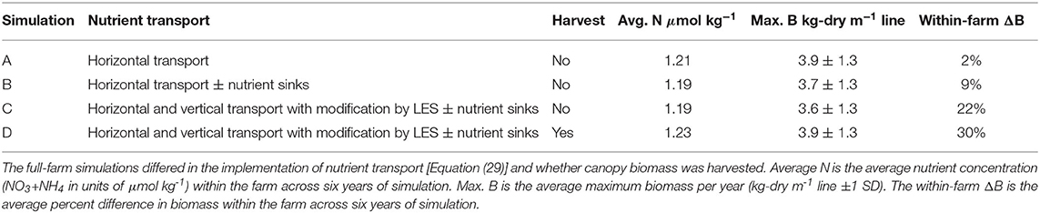
Table 2. Summary of the full-farm simulations (A–D).
The transport equation for Simulation A includes horizontal transport terms (Equation (29) terms I, II, IV, and V) but vertical transport and sink terms are set to zero (Equation (29) terms III, VI, and VII). Horizontal advection is informed by the upstream depth-varying and time-varying ROMS-BEC conditions. Transport is not modified by LES results. This simulation is most similar to current macroalgal growth models that do not incorporate within-farm hydrodynamics. The transport equation for Simulation B includes horizontal transport terms and the source and sink term specific to the nutrient being transported (Equation (29) terms I, II, IV, V, and VII), but vertical transport terms are set to zero (Equation (29) terms III and VI). The horizontal advection terms are informed by upstream depth-varying and time-varying ROMS-BEC conditions. Simulation C and D implement the full transport equation (Equation (29) terms I–VII), while Simulation C does not include kelp harvest and Simulation D does. The advection and diffusion terms are informed by upstream ROMS-BEC boundary conditions and modified by LES results using Equations (26) and (28).
Full-farm simulations are initiated by seeding growth lines with biomass equivalent to a single 1-m frond at the beginning of the year and duration is one year. Spatial resolution is 1 m3. We also perform single-day full-farm simulations to demonstrate within-farm modified nutrient fields. Within-farm transport is solved at a resolution of 30 s. Determination of total kelp nutrient uptake is conditional; re-calculated when the maximum delta-N anywhere within the farm exceeds 20%, which varies from every 10 minutes to once per day depending on upstream conditions and stage of kelp. Kelp growth and mortality are solved once per day. For Simulation D, harvest is included and reported as metric tons of fresh weight per hectare (WMT ha-1). The criteria to harvest is that there needs to be more then 2.5 WMT ha-1 available in the canopy and biomass loss exceeds growth.
3. Results
3.1. Farm-Drag Induced Modifications of Flow
Figures 4, 5 show a summary of the results from the large eddy simulation for the full canopy farm in a deep upper-mixed layer (winter conditions). The drag forces exerted by the longlines of macroalgae on the flow (Figure 4A) cause a large reduction in the horizontal flow (Figure 4B), producing mean downwelling at the leading edge of the farm. The downwelling region extends well into the farm, giving place to upwelling near the trailing edge (Figure 4E). The spatial distribution of the drag caused by the longline spacing produces a pattern of alternating fast and slow currents (note the large negative deficit within the canopy rows in Figure 4B). This crosswise shear in the streamwise velocity (approximately parallel to the longlines) is associated with a stationary pattern of vertical vorticity which, in the presence of Stokes drift promoted by surface waves, leads to pairs of counter-rotating streamwise vortices within the farm (Yan et al., 2021). These vortices are seen by the alternating pattern of upwelling and downwelling shown in the mean vertical velocity [Figure 4D, and also in Yan et al. (2021) figures 6 and 12]. Because the dynamics behind the formation of these vortices is similar to the Craik-Leibovich type II instability (Leibovich, 1983), they were termed attached Langmuir cells in Yan et al. (2021). Note that the upwelling regions tend to occur within the macroalgal rows while the downwelling is mostly located between rows. In the present farm configuration, the attached Langmuir cells extend from the top to the bottom of the farm and are present in all four LES farm simulations used here (i.e., they occur for subsurface and full canopy cases both in shallow and deep mixed layers; see Supplementary Figures 1, 3, 5).
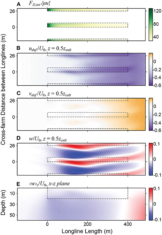
Figure 4. Mean statistics of velocity deficits from LES solution with a maximum canopy and deep mixed layer depth: (A) Magnitude of the vertically integrated drag force per unit horizontal area normalized by (B) Streamwise velocity deficit udef, normalized by the inlet bulk velocity U0; (C) Lateral velocity deficit vdef, normalized by the inlet bulk velocity U0; (D) Normalized vertical velocity w/U0 at depth z = 0.5zcult (zcult is the cultivation depth). (E) Normalized vertical velocity 〈w〉y/U0 in the x − z plane, averaged in the cross-farm y-plane. The black dashed rectangles outline the regions occupied by the kelp.
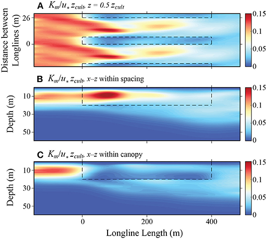
Figure 5. Mean statistics of vertical diffusivity from LES solution with a maximum canopy and deep mixed layer depth: (A) Vertical diffusivity Km, normalized by the product of the surface friction velocity u∗ and the canopy height zcult, at depth z = 0.5zcult; (B) Vertical diffusivity on the x − z plane in the spacing between adjacent canopy rows; (C) Vertical diffusivity on the x − z plane within canopy rows. The black dashed rectangles outline the regions occupied by the kelp.
In addition to these changes in the mean flow, the drag forces exerted by the macroalgae impact turbulence within the farm. Here, we quantify this effect by calculating an eddy diffusivity based on the modified K-ϵ model (Equation 27). The vertical distribution of Dv upstream of the leading edge (Figures 5B,C) is consistent with that observed in Langmuir turbulence (McWilliams et al., 1997), with a peak in the upper half of the boundary layer. As the macroalgae plants reduce the turbulence levels and increase the energy dissipation within the canopy rows, the vertical diffusivity is found to be greater in the spacing between farm rows than that in the regions occupied by canopy (Figure 5). Contrary to the mean flow patterns, the changes in diffusivity vary significantly among the different simulations. For example, simulations with subsurface canopies show a large increase in diffusivity in the upper portion of the farm (both within and between the rows; Supplementary Figures 2, 4, 6), likely produced by the strong shear layer that develops at the top of the farm in the absence of a floating dense canopy.
3.2. Results of Full-Farm Simulations
In general, there is agreement between kelp simulated by the MAG model and field observations of M. pyrifera grown on longline and from natural kelp forests in close proximity to the simulated farm. The average growth rate of MAG is 4% d-1 (Figure 3D). Also, the biomass per fronds, the distribution of biomass among fronds, the total number of fronds per plant, and the total biomass per plant agree with data from plants sampled by the Santa Barbara Coastal Long Term Ecological Research program (Figures 3B,C).
3.2.1. Within-Farm Nutrient Transport and Uptake
There are time and space-varying nutrient concentrations across the farm with key differences among simulations (Figure 6). To demonstrate the impact of heterogeneous nutrient fields on kelp uptake, one-day numerical experiments were conducted for a canopy-forming farm. We contrast two depth-averaged incoming flow conditions that have different farm-averaged residence times of seawater: (1.) 33 cm s-1 and 0.3 h residence time vs. (2.) 1.1 cm s-1 and 10 h residence time. These flow conditions represent slow and fast flow conditions at the site (Figure 2E). For each residence time, three simulations are carried out (Simulations A, B, C, described in detail in Section 2.5) that include different levels of within-farm physical transport of nutrients. Simulation A has no within-farm variation such that current speeds and nutrient concentrations are the same as the upstream boundary condition. Simulation B is similar to Simulation A, but adds within-farm macroalgal uptake of nutrients. Simulation C includes full LES-informed within-farm flows, turbulent mixing, and spatially-variable uptake of nutrients. The ROMS-BEC environmental input is depth-resolved and held static (time-invariant) for this one-day experiment. Upstream nutrient conditions are rather high (> 3 μM) within the upper mixed layer and increase rapidly at the base of the farm to more than 5 μM (Figure 6A). The LES-informed transport variables in Simulation C correspond to a maximum-canopy farm with a shallow upper mixed layer depth (i.e., MLD < zcult). In Simulation A, nutrients do not vary horizontally across the farm, because the transport equation does not include sink or vertical transport terms. Difference in uptake rates in Simulation A due to residence time are attributable to the effect of seawater velocity on the kelp uptake term (Equation (14); Figures 6F,G). For both Simulation B and C there is a farm-averaged deficit of nitrogen within the farm relative to upstream values for the short residence time runs (Figures 6B,D). The average magnitude of the deficit is similar, 3 and 5%, respectively, but for different reasons. The nutrient deficit in Simulation B is due to the drawdown of nutrients from kelp, and the nutrient deficit in Simulation C is primarily due to flow divergence around the farm in a high energy flow. Consequently, spatially integrated kelp N uptake is 5% less in Simulation B relative to Simulation A, and 3% less in Simulation C relative to Simulation A (Figure 6F). In contrast, a long residence time results in different within-farm nutrient patterns (Figures 6C,E). Simulation B has a 20% deficit in dissolved nitrogen within the farm relative to upstream conditions. Simulation C has a 16% increase in dissolved nitrogen relative to upstream conditions. Correspondingly, there is 37% and 20% less uptake in Simulations B and C, respectively, relative to Simulation A (Figure 6G). Less uptake in Simulation C despite greater nutrient concentrations is due to the effect of slowed flows resulting from kelp drag on the nutrient uptake term. Given that zcult is near the nutricline in this demonstration, nutrient concentrations within the farm increase significantly by entrainment of nutrient-rich waters from just below the farm. The degree of nutrient entrainment will be dependent on the shape of the upstream nutrient profile and the depth of the upper mixed layer.
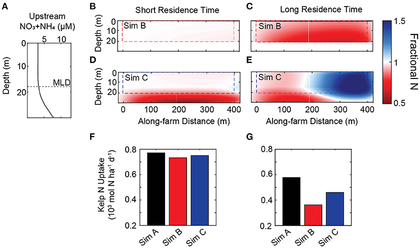
Figure 6. Effect of within-farm nutrient environment on kelp uptake. (A) Upstream nutrient profile used for both residence time demonstrations. Dashed horizontal line indicates depth of the mixed layer. Panels (B–E) illustrate the along-farm fractional change in dissolved nitrogen (NO3+NH4) between Simulations B or C relative to upstream conditions on the x − z plane with either short (0.3 h) or long (10 h) residence times on the farm. Simulation B has horizontally-homogeneous transport and kelp uptake effects on nutrient fields. Simulation C includes all within-farm physics, transport, and uptake. Values less than one indicate less dissolved nitrogen relative to upstream conditions at a given depth (red). Values greater than one indicate more dissolved nitrogen relative to upstream conditions at a given depth (blue). The dashed box outlines the region of the water-column populated with kelp (e.g., canopy-forming farm). Nutrient conditions are spatially averaged across a representative growth line (y-dimension). (F) Total daily nitrogen uptake by kelp for each simulation (spatially integrated across the entire farm and normalized to hectare) with a short residence time. (G) Total daily nitrogen uptake by kelp for each simulation with a long residence time.
3.2.2. Seasonal Modification of Farm Nutrients and Effect on Kelp Biomass
The general seasonality of the kelp is consistent among simulations and years simulated (Figure 7). A kelp canopy (defined as biomass in the top meter of the water column) is formed within approximately 100 days post-seeding. Without harvest, maximum canopy biomass occurs between late spring and summer and persists for approximately two months. Canopy shading reduces light by more than 99% at the cultivation depth relative to the surface, similar to relative light attenuation from natural kelp forests (Neushul, 1971; Gerard, 1984; Reed and Foster, 1984). The loss of kelp biomass in the fall is due to a combination of low nutrient conditions and frond senescence.
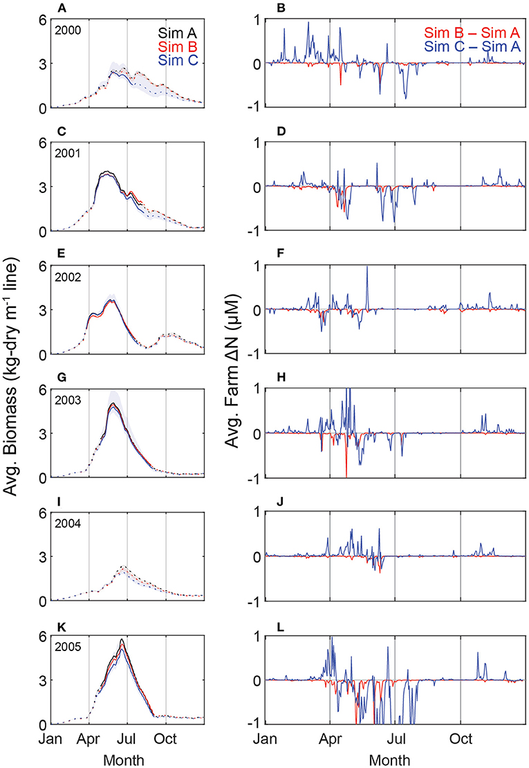
Figure 7. (Left: A,C,E,G,I,K) Daily average kelp biomass (kg-dry m-1 line) for six years of simulation. Solid line indicates a formed canopy; dashed line indicates a subsurface kelp farm. Shaded regions represent the full range of biomass across the farm. Simulation A (black line) has horizontally-homogenous transport and no loss of nutrients due to kelp uptake. Simulation B (red line) has horizontally-homogeneous transport and kelp uptake effects on nutrient fields. Simulation C (blue line) includes all within-farm physics, transport, and uptake. (Right: B,D,F,H,J,L) Daily volume-averaged difference in dissolved nitrogen (NO3+NH4) between Simulation B and Simulation A (red) and between Simulation C and Simulation A (blue). Negative values indicate lower nitrogen concentrations within the farm relative to Simulation A; positive values indicate higher nitrogen concentrations within the farm relative to Simulation A.
A canopy is formed in only four of the six years, and there is substantial inter-annual variability. Maximum annual biomass in Simulation A is 3.9 kg-dry m-1 and ranges more than 2-fold (5.8 vs. 2.4 kg-dry m-1 in 2005 and 2004, respectively). Temporal evolution of kelp biomass is similar among simulations. On average there is a 4% and 8% reduction in kelp biomass in Simulation B and Simulation C, respectively, relative to Simulation A. Volume-averaged daily nitrogen concentrations (NO3+NH4) decrease by, on average, 0.02 μM in both Simulation B and C relative to Simulation A. Simulation B has consistently lower farm-averaged nutrient concentrations than Simulation A (Figure 7), a difference than can be as much as 1 μM. While the difference in nutrients between Simulation A and C can be either negative or positive ranging from 2.5 μM less or even 1.8 μM more nutrients in Simulation C (Figure 7). The greatest reductions in farm nutrients correspond with maximum farm biomass and long residence times.
3.2.3. Spatial Differences in Kelp Biomass
Production of kelp biomass can be spatially variable across the farm and this variability is most pronounced in Simulation C where 3-D farm-induced circulation is resolved (Figure 7). Kelp performs best on the edges of the farm (Figure 8A). On average there is a 20-30% difference in within-farm biomass (Table 2) with implication for harvestable biomass. As an example, in the year 2003 harvestable biomass varies more than 3-fold across the farm, from 0.86 to more than 2.6 kg-dry m-1 line (Figure 8B). These spatial differences in productivity are attributable to patterns in farm-scale flows (see Section 3.1), where flow diverges below the farm and any replenishment of nutrients occurs downstream and near the edges of the farm. The flow-dependence of patterns in biomass suggests that there will be influence of the farm design on within-farm biomass distribution.
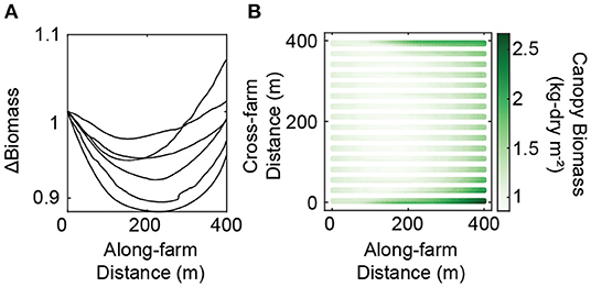
Figure 8. (A) Along-farm difference in biomass (averaged in the cross-farm, y-direction) relative to the start of the farm (x = 0) on the day of maximum biomass per year (n = 6) for full-farm Simulation C. Simulation C includes all within-farm physics, transport, and uptake. (B) Planar view of canopy biomass (kg-dry m-2) in the year 2003 on the day of maximum canopy (day of year, 149) for full-farm Simulation C.
The within-farm differences in kelp biomass for Simulation A and B are much less than that of the analysis for Simulation C. Simulation A has negligible, on average 2%, within-farm biomass differences due to slight differences in canopy shading between the middle and edge of growth lines. Simulation B has on average 9% biomass differences across the farm (Table 2).
3.2.4. Harvest Potential
A fourth simulation, Simulation D, includes criteria-based harvesting as well as full-farm feedbacks (akin to Simulation C). Simulation D predicts an average annual yield of 13 kg-wet m-1 growth line, and a total site production of 20 WMT ha-1 (Figure 9). Total annual harvested biomass ranges from 40 WMT ha-1 in 2005 to no harvest in 2000 and 2004 (because not enough canopy was generated). The number of harvests varies between no harvests and two harvests per year, with one harvest most common.
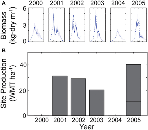
Figure 9. (A) Daily average kelp biomass (kg-dry m-1 line) for six separate years for Simulation D, which includes all within-farm physics, transport, and uptake, as well as a criteria-based harvest (harvests indicated with asterisks). Solid line indicates a formed canopy; dashed line indicates a subsurface kelp farm. Shaded regions represent the full range of biomass within the farm. Ticks on x-axis correspond with January, April, July, and October. (B) Total site production per year (metric tons of wet weight per hectare; WMT ha-1). Multiple harvests per year are stacked.
3.3. Farm-Drag Effects on the Continental Shelf
To simulate the physical effects of farm drag on the nearshore environment, we add an approximation of a vertically variable kelp-drag to ROMS. The drag force due to kelp is parameterized with Equation (5). In ROMS, FD acts as a sink on horizontal momentum.
For illustrative purposes, we choose a single frond surface area per unit volume, a(z), profile that represents a maximal kelp canopy, where frond surface area density is largest near the surface (Supplementary Table 3). For this demonstration, we also utilize a higher-resolution (Δx = 36 m) ROMS hindcast simulation of the Santa Barbara Channel without biogeochemistry, described in Dauhajre et al. (2019), that better resolves both smaller-scale, turbulent nearshore currents and farm-flow interactions as ambient currents flow through and around the farm. In this simulation, we define a 432 x 432 m farm to match the resolution of the ROMS hindcast with homogenous a(z) within the farm (Figure 2A). The hindcast spans a period of 10 days in November 2006. Continual release of a passive tracer within the farm boundaries demonstrates the effects of farm drag on local shelf flows and calculation of a “footprint” of farm effluent over the 10-day period.
Figure 10 demonstrates the effects of the (parameterized) farm drag with visualization of a passive tracer with (unitless) concentration C that is continuously released within the farm. In this manner, the tracer acts as a stand-in for any farm “effluent.” Such effluent will be advected by the shelf currents (altered by the farm itself) and may reach the shoreline or influence local ecosystem functioning. Physically, the farm drag dampens currents and causes a diversion of incoming flow beneath the farm (not shown). Additionally, the interaction of farm drag and ambient shelf currents often generates wake vortices (Figure 10A) that form downstream of the mean flow and live for hours to days. These vortices are analogous to headland wakes, exhibit large lateral shear in velocity, and influence the redistribution of farm effluent on the shelf. The snapshot in Figure 10A illustrates how these “farm wakes” advect the vertically averaged farm effluent (〈C〉z) which can reach ~ 10–15 km downstream of the farm.
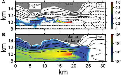
Figure 10. Local effects of a 432 x 432 x 20 m farm demonstrated with a hindcast simulation of the Santa Barbara shelf with continuous release of a passive tracer (C) in the farm (denoted by thick black lines offshore of the 60 m isobath). (A) Instantaneous snapshot of vertically averaged tracer concentration (〈C〉z, colors) and horizontal velocity (arrows, plotted every 805 m) in the upper 20 m. (B) Temporal root-mean square (over 10 days) farm “footprint” of the vertically integrated tracer (σ〈C〉z). The 10 day period samples various flow patterns with a primarily westward along-shore flow [see (A)]. In (B), the solid gray contour line denotes where farm effluent is 10% of the source. In both panels, the color-scale is normalized by the maximum value within the farm. Note the farm-drag induced wake vortices of the farm effluent (A) and approximate 20 km extent of the effluent footprint (B).
A time-averaged view of the farm effluent distribution shows a substantial farm “footprint” due to a primarily westward, along-shore flow during the 10-day simulation period. We plot this footprint as the temporal root-mean square of the vertically integrated tracer concentration in the upper 20 m (σ〈C〉z, where 〈.〉 denotes a 10-day temporal root-mean square), shown in Figure 10B. Generally, the farm effluent extends upcoast (westward) of the farm, due to the predominance of a large-scale, westward along-shore flow. However, as the snapshot (Figure 10A) illustrates, more complex, smaller-scale flow patterns ultimately contribute to the mean distribution of farm effluent. Notably, 10% of the total released effluent (solid gray line, Figure 10B) extends ~ 20 km in the along-shore direction. This relatively large footprint suggests non-trivial, significant affects of the farm on the continental shelf environment due to a combination of local flow alteration by drag and associated transport of farm by-products on the shelf. While we limit the analysis here to a fully grown stage farm with a large canopy on the surface, we observe similar footprints for other a(z) profiles with reduced surface canopy. Similarly, we leave more detailed investigation of local ecosystem effects, with a coupled ROMS-BEC-MAG model, for future study.
4. Discussion
Here, we demonstrate that resolving within-farm physical circulation and chemical fields in a numerical model impacts predicted within-farm kelp biomass. Macrocystis pyrifera is a large seaweed with substantial ability to modify the circulation and chemistry of the surrounding water, and this modified environment affects kelp growth (Figure 1B). Many processes can influence kelp production regardless of being in a natural or farmed setting. Canopy shading attenuates light and thus affects kelp growth at depth, nutrient drawdown decreases nitrogen available for uptake, and slowed flow due to kelp drag decreases uptake rates because of thicker diffusive boundary layers. The MACMODS modeling framework resolves these processes, predicts spatial and temporal heterogeneity in farm production, and thus should allow for a more accurate assessment of overall farm performance.
We apply MACMODS to simulate a M. pyrifera farm near Santa Barbara, California. The model predicts significant flow divergence both beneath and around the farm (Figure 4). Overall, this has minimal impact on predictions of average farm kelp biomass (< 10%), but has substantial impact on day-to-day farm nutrient conditions (Figures 6, 7) and within-farm biomass distribution (Figure 8). By combining fine-scale within-farm circulation (LES) with regional ocean conditions (ROMS) we find that nutrient concentrations can be more than or less than upstream nutrients due to a combination of nutrient drawdown via kelp uptake, flow divergence of high nutrients below and around the farm in fast flows, and replenishment of nutrients at the trailing edge of the farm (Figure 6). We also find shear-driven turbulence at the base of the suspended kelp farm (Figure 5) and Langmuir-like attached eddies on the vertical scale of the kelp canopy (Figure 4) together serve to passively entrain nutrients from waters below the farm that partially negate the negative effects of nutrient drawdown due to kelp uptake (Figure 6). However, given that zcult is near the nutricline in this demonstration, nutrient concentrations within the farm can increase by entrainment of nutrient-rich waters from just below the farm. The degree of nutrient entrainment will be dependent on the shape of the upstream nutrient profile and the depth of the upper mixed layer. Therefore, results will be sensitive to site location. If the depth of the upper mixed layer (unstratified region with typically lower nutrient concentrations) is much deeper than the depth of the farm, there is less opportunity for any modification of within-farm nutrients other than replenishment of nutrient loss from kelp uptake.
Similar models of macroalgae growth have been well validated against observations for different species (Jackson, 1987; Solidoro et al., 1997; Aldridge and Trimmer, 2009; Broch and Slagstad, 2012; Hadley et al., 2015). Given the lack of farm-scale observations for M. pyrifera in the Southern California Bight, we compared the macroalgal growth model to observations from a nearby natural kelp forest. Predicted biomass and growth rates fall within the range of observations (Figure 3). The farm circulation patterns predicted by LES also need to be compared with and validated against farm-scale observations. Altered flows are likely to be modified by farm design (e.g., longline spacing, planting depth), canopy structure (e.g., stage of growth, stocking density), and ocean conditions such as the depth of the upper mixed layer and nutricline, surface wave forcing, and farm orientation to mean flow. The intention of developing this modeling framework is for it to be flexible and readily adapted to other regions and species. The requirements for successful implementation of MACMODS are knowledge of the regional setting with local flow, temperature, salinity and nutrient conditions, along with known drag and growth model characteristics of the species to be modeled (e.g., Table 1) in order to parameterize and implement both LES and MAG, and known farm design parameters (e.g., farm size and position of seaweed growth lines within the farm).
Further comparisons can be made between predictions of yield by our modeled farm and yields from other kelp farms around the world. Average annual yield from our full-farm Simulation D is 13 kg-wet m-1 line (Figure 9). Kelp farms of Saccharina latissima in China are estimated to yield up to 22.9 kg-wet m-1 line (Campbell et al., 2019), and estimates for S. latissima farms in Europe are around 9.1 to 16 kg-wet m-1 line (Peteiro and Freire, 2013; Seghetta et al., 2016). Stocking density, the amount of growing line per m2 of cultivation area, generate large differences in site production. For example, grid systems employed in China densely pack seaweed cultivation to a stocking density of approximately 0.66 mm-2 (Shi et al., 2011). Overall site production is thus 151 WMT ha-1. The cultivation system simulated here for M. pyrifera has a stocking density of 0.16 mm-2, resulting in an overall site production of 20 WMT ha-1. To achieve greater stocking densities more effective cultivation infrastructure will need to be employed so that growth lines can cover more area within the farm but limits will be species and location specific.
There is expanding interest in the potential of macroalgal cultivation for carbon sequestration. Our estimates of site production at 20 WMT ha−1 is equivalent to 0.6 tons C ha−1 (with a dry-to-wet weight ratio of 0.094 and 32% carbon in algal tissue; Supplementary Table 1). We caution that this estimate of harvested C can range from 0.4 to 0.9 tons C ha−1. The percent of carbon in M. pryifera is on average 32% and can actually be as low as 20% or as high as 45% (Rassweiler et al., 2018). A dynamic model that simulates both carbon and nitrogen will be of great utility to quantify carbon removed via harvesting as well as carbon exported to the surrounding coastal system whether as particulate or dissolved matter.
There is a history of varying success of suspended cultivation attempts for M. pyrifera dating back to the 1970's (Kim et al., 2019). Our findings suggest that yields can be improved when farm installation considers orientation relative to flow (i.e., longlines oriented parallel to the dominant flow direction), spacing of longlines in the cross-farm direction, and site selection based on the depth of the upper mixed layer (i.e., a seasonal nutricline in close proximity to the cultivation depth, Figure 2F). Farming of M. pyrifera in Chile in suspended systems has been demonstrated to be feasible (Camus et al., 2018, 2019). Challenges experienced by these farms include pests and diseases not explicitly modeled here. Such processes should be included in farm monitoring plans along with other sources of loss not included in our model such as entanglement and big-wave events leading to whole-plant loss.
Natural kelp beds are highly productive with a vast majority of biomass entering nearby and distant food webs as detritus (Krumhansl and Scheibling, 2012). Detritus may be consumed within or adjacent to the kelp by herbivores and detritivores, transported into deeper habitat below the photic zone (Vanderklift and Wernberg, 2008; Britton-Simmons et al., 2012), or deposited on shore as beach wrack (Dugan et al., 2011). For farming, similar farm-environment interactions are anticipated, and the amount and fate of farm-based kelp detritus, whether as particulate or dissolved organic matter, warrants further development and exploration [Equations (12), (13)]. The MACMODS framework presented here allows for such investigation but is beyond the scope of the within-farm analysis. Still, exploration of farm-drag effects on coastal circulation offers insight into the potential spatial extent of physicochemical environmental changes caused by the farm (Figure 10), and raises the possibility of farm-farm interactions to be further explored. In the same context, changes in planktonic communities are possible with large-scale farming as phytoplankton experience increased competition for light and nutrients from cultivated species (Shi et al., 2011). Other ecosystem implications to be explored include, for example, whether added kelp detritus could accelerate subsurface respiration and remineralization. Exploration of these topics, including natural and farmed kelp, will require coupling of the macroalgal growth model with an eddy-resolving oceanic physical-biogeochemical model (ROMS-BEC in this case).
As we reckon with the growing costs of climate change, interest in “living” solutions is burgeoning, such as seaweed cultivation to produce cleaner fuels, to remediate marine ecosystems, to provide a sustainable food source, and as a strategy for removing carbon from the atmosphere to minimize future damage to our earth systems. There is a growing need for computational tools to help gauge the feasibility and scalability of seaweed cultivation as a potential solution and to predict potential environmental costs and benefits of large-scale seaweed cultivation. Biophysical models, such as MACMODS, can be used alongside techno-economic analysis to better understand the financial viability of seaweed farming under different environmental policy scenarios (e.g., nutrient credits or a carbon tax). Seed selection for specific biological characteristics can improve farm yields, and growth models can be used to enable predictions for performance of different traits among environments.
Data Availability Statement
The datasets presented in this study can be found in online repositories. The names of the repository/repositories and accession number(s) can be found at: https://github.com/macmods/mag3-mp/releases/tag/v1.
Author Contributions
CF and CY: data curation, formal analysis, methodology, validation, visualization, original draft, and editing. MC: conceptualization, funding acquisition, methodology, supervision, validation, visualization, original draft, and editing. DD: data curation, formal analysis, methodology, visualization, original draft, and editing. JM: conceptualization, funding acquisition, methodology, resources, supervision, validation, and editing. JI: conceptualization, funding acquisition, methodology, validation, and editing. MM: methodology, validation, and editing. RK and MS: conceptualization, funding acquisition, supervision, and editing. FK: data curation, formal analysis, methodology, and editing. IA-S: methodology, validation, and editing. KD: conceptualization, lead funding acquisition, project administration, resources, supervision, and editing.
Funding
This project was supported by the U.S. Department of Energy ARPA-E's MARINER (Macroalgae Research Inspiring Novel Energy Resources) program, grant number DE-AR0000920.
Conflict of Interest
JI was employed by Patagonia Seaweeds.
The remaining authors declare that the research was conducted in the absence of any commercial or financial relationships that could be construed as a potential conflict of interest.
Publisher's Note
All claims expressed in this article are solely those of the authors and do not necessarily represent those of their affiliated organizations, or those of the publisher, the editors and the reviewers. Any product that may be evaluated in this article, or claim that may be made by its manufacturer, is not guaranteed or endorsed by the publisher.
Supplementary Material
The Supplementary Material for this article can be found online at: https://www.frontiersin.org/articles/10.3389/fmars.2022.752951/full#supplementary-material
References
Aldridge, J., and Trimmer, M. (2009). “Modelling the distribution and growth of ‘problem’ green seaweed in the Medway Estuary, UK,” in Eutrophication in Coastal Ecosystems Dordrecht: Springer, 107–122.
Arnold, K. E., and Manley, S. L. (1985). Carbon allocation in Macrocystis pyrifera (phaeophyte): intrinsic variability in photosynthesis and respiration. J. Phycol. 21, 154–167.
Belcher, S. E., Grant, A. L., Hanley, K. E., Fox-Kemper, B., Van Roekel, L., Sullivan, P. P., et al. (2012). A global perspective on Langmuir turbulence in the ocean surface boundary layer. Geophys. Res. Lett. 39, L18605. doi: 10.1029/2012GL052932
Bell, T. W., Reed, D. C., Nelson, N. B., and Siegel, D. A. (2018). Regional patterns of physiological condition determine giant kelp net primary production dynamics. Limnol. Oceanography 63, 472–483. doi: 10.1002/LNO.10753
Bou-Zeid, E., Meneveau, C., and Parlange, M. B. (2005). A scale-dependent Lagrangian dynamic model for large eddy simulation of complex turbulent flows. Phys. Fluids 17, 025105. doi: 10.1063/1.1839152
Britton-Simmons, K. H., Rhoades, A. L., Pacunski, R. E., Galloway, A. W., Lowe, A. T., Sosik, E. A., et al. (2012). Habitat and bathymetry influence the landscape-scale distribution and abundance of drift macrophytes and associated invertebrates. Limnol. Oceanography 57, 176–184. doi: 10.4319/lo.2012.57.1.0176
Broch, O. J., and Slagstad, D. (2012). Modelling seasonal growth and composition of the kelp Saccharina latissima. J. Appl. Phycol. 24, 759–776. doi: 10.1007/s10811-011-9695-y
Brzezinski, M. A., Reed, D. C., Harrer, S., Rassweiler, A., Melack, J. M., Goodridge, B. M., et al. (2013). Multiple sources and forms of nitrogen sustain year-round kelp growth on the inner continental shelf of the santa barbara channel. Oceanography 26, 114–123. doi: 10.5670/oceanog.2013.53
Buschmann, A., Vásquez, J., Osorio, P., Reyes, E., Filún, L., Hernández-González, M., et al. (2004). The effect of water movement, temperature and salinity on abundance and reproductive patterns of Macrocystis spp. (Phaeophyta) at different latitudes in Chile. Marine Biol. 145, 849–862. doi: 10.1007/S00227-004-1393-8
Campbell, I., Macleod, A., Sahlmann, C., Neves, L., Funderud, J., Øverland, M., et al. (2019). The environmental risks associated with the development of seaweed farming in Europe-prioritizing key knowledge gaps. Front. Marine Sci. 6, 107. doi: 10.3389/fmars.2019.00107
Camus, C., Infante, J., and Buschmann, A. H. (2018). Overview of 3 year precommercial seafarming of Macrocystis pyrifera along the Chilean coast. Rev. Aquacul. 10, 543–559. doi: 10.1111/RAQ.12185
Camus, C., Infante, J., and Buschmann, A. H. (2019). Revisiting the economic profitability of giant kelp Macrocystis pyrifera (Ochrophyta) cultivation in Chile. Aquaculture 502, 80–86. doi: 10.1016/j.aquaculture.2018.12.030
Cariboni, J., Gatelli, D., Liska, R., and Saltelli, A. (2007). The role of sensitivity analysis in ecological modelling. Ecol. Model. 203, 167–182. doi: 10.1016/j.ecolmodel.2005.10.045
Chamecki, M., Chor, T., Yang, D., and Meneveau, C. (2019). Material transport in the ocean mixed layer: recent developments enabled by large eddy simulations. Rev. Geophys. 57, 1338–1371. doi: 10.1029/2019RG000655
Chen, S., Xu, K., Ji, D., Wang, W., Xu, Y., Chen, C., and Xie, C. (2020). Release of dissolved and particulate organic matter by marine macroalgae and its biogeochemical implications. Algal Research, 52:102096.
Craik, A. D. D. and Leibovich, S. (1976). A rational model for Langmuir circulations. Journal of Fluid Mechanics, 73(3):401–426.
Dauhajre, D. P., McWilliams, J. C., and Renault, L. (2019). Nearshore Lagrangian connectivity: submesoscale influence and resolution sensitivity. J. Geophys. Res. Oceans 124, 5180–5204. doi: 10.1029/2019JC014943
Dean, T. A., and Jacobsen, F. R. (1984). Growth of juvenile Macrocystis pyrifera (Laminariales) in relation to environmental factors. Marine Biol. 83, 301–311.
Delaux, S., Stevens, C. L., and Popinet, S. (2011). High-resolution computational fluid dynamics modelling of suspended shellfish structures. Environ. Fluid Mech. 11, 405–425. doi: 10.1007/s10652-010-9183-y
Deutsch, C., Frenzel, H., McWilliams, J. C., Renault, L., Kessouri, F., Howard, E., et al. (2021). Biogeochemical variability in the California Current System. Progr. Oceanography 196, 102565. doi: 10.1016/j.pocean.2021.102565
Duarte, C. M., Wu, J., Xiao, X., Bruhn, A., and Krause-Jensen, D. (2017). Can seaweed farming play a role in climate change mitigation and adaptation? Front. Marine Sci. 4, 100. doi: 10.3389/fmars.2017.00100
Dugan, J. E., Hubbard, D. M., Page, H. M., and Schimel, J. P. (2011). Marine macrophyte wrack inputs and dissolved nutrients in beach sands. Estuaries Coasts 34, 839–850. doi: 10.1007/S12237-011-9375-9
FAO (2018). The global status of seaweed production, trade and utilization. Globefish Res. Programme 124:I.
Fernand, F., Israel, A., Skjermo, J., Wichard, T., Timmermans, K. R., and Golberg, A. (2017). Offshore macroalgae biomass for bioenergy production: Environmental aspects, technological achievements and challenges. Renew. Sustain. Energy Rev. 75, 35–45. doi: 10.1016/j.rser.2016.10.046
Froehlich, H. E., Afflerbach, J. C., Frazier, M., and Halpern, B. S. (2019). Blue growth potential to mitigate climate change through seaweed offsetting. Curr. Biol. 29, 3087–3093.e3. doi: 10.1016/j.cub.2019.07.041
Gaylord, B., Rosman, J. H., Reed, D. C., Koseff, J. R., Fram, J., MacIntyre, S., et al. (2007). Spatial patterns of flow and their modification within and around a giant kelp forest. Limnol. Oceanography 52, 1838–1852. doi: 10.4319/LO.2007.52.5.1838
Gerard, V. A. (1982). In situ rates of nitrate uptake by giant kelp, Macrocystis pyrifera (L.) C. Agardh: tissue differences, environmental effects, and predictions of nitrogen-limited growth. J. Exp. Marine Biol. Ecol. 62, 211–224.
Gerard, V. A. (1984). The light environment in a giant kelp forest: Influence of Macrocystis pyrifera on spatial and temporal variability. Marine Biol. 84, 189–195.
Hadley, S., Wild-Allen, K., Johnson, C., and Macleod, C. (2015). Modeling macroalgae growth and nutrient dynamics for integrated multi-trophic aquaculture. J. Appl. Phycol. 27, 901–916. doi: 10.1007/s10811-014-0370-y
Haines, K. C., and Wheeler, P. A. (1978). Ammonium and nitrate uptake by the marine macrophytes Hypnea musvuformis (Rhodophyta) and Macrocystis pyrifera (Phaeophyta). J. Phycol. 14, 319–324.
Harrison, P. J., and Hurd, C. L. (2001). Nutrient physiology of seaweeds: application of concepts to aquaculture. Cahiers de Biologie Marine 42, 71–82.
Henderson, S. M. (2019). Motion of buoyant, flexible aquatic vegetation under waves: simple theoretical models and parameterization of wave dissipation. Coastal Engineering, 152:103497. doi: 10.1016/j.coastaleng.2019.04.009
Hepburn, C. D., Holborow, J. D., Wing, S. R., Frew, R. D., and Hurd, C. L. (2007). Exposure to waves enhances the growth rate and nitrogen status of the giant kelp Macrocystis pyrifera. Marine Ecol. Progr. Series 339, 99–108. doi: 10.3354/MEPS339099
Hoegh-Guldberg, O., Caldeira, K., Chopin, T., Gaines, S., Haugen, P., Hemer, M., et al. (2019). The Ocean as a Solution to Climate Change: Five Opportunities for Action. Technical Report. Washington, DC: World Resources Institute. Available online at: http://www.oceanpanel.org/climate
Hurd, C. L. (2017). Shaken and stirred: the fundamental role of water motion in resource acquisition and seaweed productivity. Perspect. Phycol. 4, 73–81. doi: 10.1127/pip/2017/0072
Hurd, C. L., Harrison, P. J., Bischof, K., and Lobban, C. S. (2014). Seaweed Ecology and Physiology, Second Edition. Cambridge, Cambridge University Press.
Jackson, G. A. (1987). Modelling the growth and harvest yield of the giant kelp Macrocystis pyrifera. Marine Biol. 95, 611–624.
Jackson, G. A. (1997). Currents in the high drag environment of a coastal kelp stand off California. Continental Shelf Res. 17, 1913–1928.
Katul, G. G., Mahrt, L., Poggi, D., and Sanz, C. (2004). One-and two-equation models for canopy turbulence. Boundary Layer Meteorol. 113, 81–109. doi: 10.1023/B:BOUN.0000037333.48760.e5
Kessouri, F., Bianchi, D., Renault, L., McWilliams, J. C., Frenzel, H., and Deutsch, C. A. (2020). Submesoscale currents modulate the seasonal cycle of nutrients and productivity in the California Current System. Glob. Biogeochem. Cycles 34, e2020GB006578. doi: 10.1029/2020GB006578
Kim, J., Stekoll, M., and Yarish, C. (2019). Opportunities, challenges and future directions of open-water seaweed aquaculture in the United States. Phycologia 58, 446–461. doi: 10.1080/00318884.2019.1625611
Kopczak, C. D. (1994). Variability of nitrate uptake capacity in Macrocystis pyrifera (Lamineriales, Phaeophyta) with nitrate and light availability. J. Phycol. 30, 573–580.
Krumhansl, K. A., and Scheibling, R. E. (2012). Production and fate of kelp detritus. Marine Ecol. Progr. Series 467, 281–302. doi: 10.3354/MEPS09940
Large, W. G., McWilliams, J. C., and Doney, S. C. (1994). Oceanic vertical mixing: a review and a model with a nonlocal boundary layer parameterization. Rev. Geophys. 32, 363–403.
Leibovich, S. (1983). The form and dynamics of Langmuir circulations. Ann. Rev. Fluid Mech. 15, 391–427.
Lorenzen, C. J. (1972). Extinction of light in the ocean by phytoplankton. ICES J. Marine Sci. 34, 262–267.
Luhar, M., and Nepf, H. M. (2011). Flow-induced reconfiguration of buoyant and flexible aquatic vegetation. Limnol. Oceanography 56, 2003–2017. doi: 10.4319/lo.2011.56.6.2003
Mason, E., Molemaker, J., Shchepetkin, A. F., Colas, F., McWilliams, J. C., and Sangrà, P. (2010). Procedures for offline grid nesting in regional ocean models. Ocean Model. 35, 1–15. doi: 10.1016/J.OCEMOD.2010.05.007
McWilliams, J. C. (2016). Submesoscale currents in the ocean. Proc. R. Soc. A Math. Phys. Eng. Sci. 472, 20160117. doi: 10.1098/rspa.2016.0117
McWilliams, J. C., Sullivan, P., and Moeng, C. (1997). Langmuir turbulence in the ocean. J. Fluid Mech. 334, 1–30.
Navarrete, I. A., Kim, D. Y., Wilcox, C., Reed, D. C., Ginsburg, D. W., Dutton, J. M., et al. (2021). Effects of depth-cycling on nutrient uptake and biomass production in the giant kelp Macrocystis pyrifera. Renew. Sustain. Energy Rev. 141, 110747. doi: 10.1016/j.rser.2021.110747
Neushul, M. (1971). Submarine illumination in Macrocystis beds. Nova Hedwigia. Beihefte 32, 241–254.
Nyman, M. A., Brown, M. T., Neushul, M., Harger, B. W. W., and Keogh, J. A. (1993). Mass distribution in the fronds of Macrocystis pyrifera from New Zealand and California. Hydrobiologia 260–261, 57–65.
Parker, B. C. (1965). Translocation in the giant kelp Macrocystis I. rates, direction, quantity of C14-labeled products and fluorescein. J. Phycol. 1, 41–46.
Peteiro, C., and Freire, Ó. (2011). Effect of water motion on the cultivation of the commercial seaweed Undaria pinnatifida in a coastal bay of Galicia, Northwest Spain. Aquaculture 314, 269–276. doi: 10.1016/j.aquaculture.2011.02.009
Peteiro, C., and Freire, Ó. (2013). Biomass yield and morphological features of the seaweed Saccharina latissima cultivated at two different sites in a coastal bay in the Atlantic coast of Spain. J. Appl. Phycol. 25, 205–213. doi: 10.1007/s10811-012-9854-9
Plew, D. R. (2011). Shellfish farm-induced changes to tidal circulation in an embayment, and implications for seston depletion. Aquacult. Environ. Interact. 1, 201–214. doi: 10.3354/aei00020
Plew, D. R., Spigel, R. H., Stevens, C. L., Nokes, R. I., and Davidson, M. J. (2006). Stratified flow interactions with a suspended canopy. Environ. Fluid Mech. 6, 519–539. doi: 10.1007/s10652-006-9008-1
Plew, D. R., Stevens, C. L., Spigel, R. H., and Hartstein, N. D. (2005). Hydrodynamic implications of large offshore mussel farms. IEEE J. Oceanic Eng. 30, 95–108. doi: 10.1109/JOE.2004.841387
Rassweiler, A., Reed, D. C., Harrer, S. L., and Nelson, J. C. (2018). Improved estimates of net primary production, growth, and standing crop of Macrocystis pyrifera in Southern California. Ecology 99, 2132. doi: 10.1002/ecy.2440
Reed, D., and Rassweiler, A. (2018). SBC LTER: REEF: Allometric Measurements of Giant Kelp Ver 1. Technical Report, Environmental Data Initiative. Available online at: https://doi.org/10.6073/pasta/e880e6b231af718c63f623893c678c86 (accessed November 28, 2020).
Reed, D. C., and Foster, M. S. (1984). The effects of canopy shadings on algal recruitment and growth in a giant kelp forest. Ecology 65, 937–948.
Renault, L., McWilliams, J. C., Kessouri, F., Jousse, A., Frenzel, H., Chen, R., et al. (2021). Evaluation of high-resolution atmospheric and oceanic simulations of the California current system. Progr. Oceanography 195, 102564. doi: 10.1016/j.pocean.2021.102564
Rodriguez, G. E., Rassweiler, A., Reed, D. C., and Holbrook, S. J. (2013). The importance of progressive senescence in the biomass dynamics of giant kelp (Macrocystis pyrifera). Ecology 94, 1848–1858. doi: 10.1890/12-1340.1
Roleda, M. Y., and Hurd, C. L. (2019). Seaweed nutrient physiology: application of concepts to aquaculture and bioremediation. Phycologia 58, 552–562. doi: 10.1080/00318884.2019.1622920
Schiel, D. R., and Foster, M. S. (2015). The Biology and Ecology of Giant Kelp Forests. Oakland, CA: University of California Press.
Schmitz, K., and Lobban, C. S. (1976). A survey of translocation in laminariales (phaeophyceae). Marine Biol. 36, 207–216.
Seghetta, M., Hou, X., Bastianoni, S., Bjerre, A.-B., and Thomsen, M. (2016). Life cycle assessment of macroalgal biorefinery for the production of ethanol, proteins and fertilizers–a step towards a regenerative bioeconomy. J. Cleaner Prod. 137, 1158–1169. doi: 10.1016/J.JCLEPRO.2016.07.195
Shchepetkin, A. F., and McWilliams, J. C. (2005). The regional oceanic modeling system (ROMS): a split-explicit, free-surface, topography-following-coordinate oceanic model. Ocean Model. 9, 347–404. doi: 10.1016/j.ocemod.2004.08.002
Shi, J., Wei, H., Zhao, L., Yuan, Y., Fang, J., and Zhang, J. (2011). A physical-biological coupled aquaculture model for a suspended aquaculture area of China. Aquaculture 318, 412–424.
Sipler, R. E., and Bronk, D. A. (2015). “Dynamics of dissolved organic nitrogen,” in Biogeochemistry of Marine Dissolved Organic Matter: Second Edition. San Diego, CA: Elsevier Inc., 127–232.
Skamarock, W. C., Klemp, J. B., Dudhia, J. B., Gill, D. O., Barker, D. M., Duda, M. G., et al. (2008). A Description of the Advanced Research WRF Version 3. NCAR Technical Note TN-475+STR.
Skyllingstad, E. D., and Denbo, D. W. (1995). An ocean large-eddy simulation of Langmuir circulations and convection in the surface mixed layer. J. Geophys. Res. Oceans 100, 8501–8522.
Smith, J. M., Brzezinski, M. A., Melack, J. M., Miller, R. J., and Reed, D. C. (2018). Urea as a source of nitrogen to giant kelp (Macrocystis pyrifera). Limnol. Oceanography Lett. 3, 365–373.
Solidoro, C., Pecenik, G., Pastres, R., Franco, D., and Dejak, C. (1997). Modelling macroalgae (Ulva rigida) in the Venice lagoon: Model structure identification and first parameters estimation. Ecol. Model. 94, 191–206.
Stevens, C. L., and Hurd, C. L. (1997). Boundary-layers around bladed aquatic macrophytes. Hydrobiologia 346, 119–128.
Utter, B., and Denny, M. (1996). Wave-induced forces on the giant kelp Macrocystis pyrifera (Agardh): Field test of a computational model. J. Expe. Biol. 199, 2645–2654.
Vanderklift, M. A., and Wernberg, T. (2008). Detached kelps from distant sources are a food subsidy for sea urchins. Oecologia 157, 327–335. doi: 10.1007/s00442-008-1061-7
Wang, B., Cao, L., Micheli, F., Naylor, R. L., and Fringer, O. B. (2018). The effects of intensive aquaculture on nutrient residence time and transport in a coastal embayment. Environ. Fluid Mech. 18, 1321–1349. doi: 10.1007/s10652-018-9595-7
Wheeler, P. A., and North, W. J. (1980). Effect of nitrogen supply on nitrogen content and growth rate of juvenile Macrocstis pyrifera (Phaeophyta) sporophytes. J. Phycol. 16, 577–582.
Yan, C., McWilliams, J., and Chamecki, M. (2021). Generation of attached Langmuir circulations by a suspended macroalgal farm. J. Fluid Mech. 915, A76. doi: 10.1017/jfm.2021.111
Yang, D., Chen, B., Chamecki, M., and Meneveau, C. (2015). Oil plumes and dispersion in Langmuir, upper-ocean turbulence: Large-eddy simulations and k-profile parameterization. J. Geophys. Res. Oceans 120, 4729–4759. doi: 10.1002/2014JC010542
Yuan-Hui, L., and Gregory, S. (1974). Diffusion of ions in sea water and in deep-sea sediments. Geochimica et Cosmochimica Acta 38, 703–714.
Zhang, J., Wu, W., Ren, J., and Lin, F. (2016). A model for the growth of mariculture kelp Saccharina japonica in Sanggou Bay, China. Aquacult. Environ. Interact. 8, 273–283. doi: 10.3354/AEI00171
Zhou, J., and Venayagamoorthy, S. K. (2019). Near-field mean flow dynamics of a cylindrical canopy patch suspended in deep water. J. Fluid Mech. 858, 634–655. doi: 10.1017/jfm.2018.775
Zimmerman, R., and Kremer, J. (1986). In situ growth and chemical composition of the giant kelp, Macrocystis pyrifera: Response to temporal changes in ambient nutrient availability. Marine Ecol. Progr. Series 27, 277–285.
Keywords: Macrocystis pyrifera, large eddy simulation, macroalgal growth model, seaweed farming, farm-environment interactions
Citation: Frieder CA, Yan C, Chamecki M, Dauhajre D, McWilliams JC, Infante J, McPherson ML, Kudela RM, Kessouri F, Sutula M, Arzeno-Soltero IB and Davis KA (2022) A Macroalgal Cultivation Modeling System (MACMODS): Evaluating the Role of Physical-Biological Coupling on Nutrients and Farm Yield. Front. Mar. Sci. 9:752951. doi: 10.3389/fmars.2022.752951
Received: 03 August 2021; Accepted: 03 February 2022;
Published: 03 March 2022.
Edited by:
David Koweek, Ocean Visions, Inc., United StatesReviewed by:
Margaux Filippi, Open Earth Foundation, United StatesScott Hadley, University of Tasmania, Australia
Mar Fernández-Méndez, Helmholtz Association of German Research Centres (HZ), Germany
Copyright © 2022 Frieder, Yan, Chamecki, Dauhajre, McWilliams, Infante, McPherson, Kudela, Kessouri, Sutula, Arzeno-Soltero and Davis. This is an open-access article distributed under the terms of the Creative Commons Attribution License (CC BY). The use, distribution or reproduction in other forums is permitted, provided the original author(s) and the copyright owner(s) are credited and that the original publication in this journal is cited, in accordance with accepted academic practice. No use, distribution or reproduction is permitted which does not comply with these terms.
*Correspondence: Kristen A. Davis, ZGF2aXNAdWNpLmVkdQ==