Seasonal Variability of the Carbonate System and Air–Sea CO2 Flux in the Outer Changjiang Estuary, East China Sea

Three field surveys were conducted in the outer Changjiang Estuary on the inner shelf of the East China Sea in March, July, and October, 2018. Observations of total-scale pH (pH_T), total alkalinity (A_T), and calculated total dissolved inorganic carbon (C_T), the partial pressure of CO₂ (pCO₂), and the air–sea CO₂ exchange flux (FCO₂) were studied in the surface waters. The results showed that the Changjiang Diluted Water (CDW) area was a source of atmospheric CO₂ in July and October (4.97 and 8.67 mmol CO₂/m²/day, respectively). The oversaturation of CO₂ was mainly ascribed to the respiration of terrestrial organic and inorganic materials sourced from the Changjiang River discharge, overwhelming the CO₂ uptake due to primary productivity despite the high phytoplankton biomass in summer. The air–sea CO₂ flux was greater in October than in July in the CDW, which is attributed to the increasing wind speed. In contrast, the Yellow Sea Water (YSW) and the East China Sea Shelf Water (ECSSW) were a weak CO₂ sink in March (–0.71 and –2.86 mmol CO₂/m²/day, respectively) and July (–1.28 mmol CO₂/m²/day in the ECSSW) following the CO₂ uptake of phytoplankton production, however, they were a CO₂ source by October (3.30 mmol CO₂/m²/day in the YSW and 1.18 mmol CO₂/m²/day in the ECSSW). The cooling effect during the cold season reduced the sea surface pCO₂, resulting in a CO₂ sink in the CDW, YSW, and ECSSW areas in March. However, the regions became a source of atmospheric CO₂ in October, possibly driven by vertical mixing, which brought C_T-enriched bottom water to the surface and increased the pCO₂. The study region was a net CO₂ sink in March and a net CO₂ source in July and October with an average FCO₂ of –1.25, 1.71, and 3.06 mmol CO₂/m²/day, respectively.

Introduction

Although coastal systems contribute only a small percentage of the global ocean surface area (a little over 7%), they play a disproportionately important role in the global carbon cycle and ultimately affect global climate change processes (Chen et al., 2013). The annual mean for the net CO₂ uptake by the global ocean is estimated to be –2.5 ± 0.6 GtC/year (Friedlingstein et al., 2019), in which marginal seas absorb approximately 8–18% of CO₂ (0.2–0.45 GtC/year) (Borges et al., 2005; Laruelle et al., 2010; Cai, 2011). Coastal margins are the most heterogeneous areas of the oceans in the world, with strongly contrasting physical and biogeochemical activity (Cai and Dai, 2004; Borges et al., 2005). The air–sea CO₂ flux (FCO₂) in global marginal seas is still a matter of debate, although field surveys and models show that they generally act as a net atmospheric CO₂ sink (Chen and Borges, 2009; Bauer et al., 2013).

Coastal systems can be classified into two distinct physical–biogeochemical groups: ocean-dominated margins (OceMars) (Dai et al., 2013); and river-dominated ocean margins (RioMars) (McKee et al., 2004). OceMars exchanges with the open ocean through the horizontal intrusion of water masses, vertical mixing, and upwelling. Their CO₂ sink/source status mainly depends on the balance between C_T/nutrients imported from the open ocean and the subsequent biological consumption in the euphotic zone (Dai et al., 2013). However, RioMars are greatly affected by significant riverine inputs of dissolved and particulate terrestrial material (McKee et al., 2004). Generally, they act as a CO₂ sink at high river discharges, because the CO₂ consumed by biological production exceeds the CO₂ produced by the decomposition of terrestrial organic matter (Cao et al., 2011; Tseng et al., 2011; Guo et al., 2012).

The East China Sea (ECS) is one of the broadest marginal seas in the world and is characterized by high biological production. Since the 1990s, the carbonate dynamics of the ECS have been extensively studied, and indications are that it is a net CO₂ sink (Tsunogai et al., 1997, 1999; Shim et al., 2007; Chou et al., 2009, 2011, 2013; Guo et al., 2015). The ECS shelf may absorb as much as 0.013–0.030 GtC/year (Wang et al., 2000). Due to the high Changjiang River discharge, the ECS is a typical river-dominated coastal system in summer, where it acts as a net CO₂ sink (Chou et al., 2017). However, the ECS has seasonal and spatial variations in CO₂ flux and is a moderate or large net atmospheric CO₂ sink throughout the year, except in autumn (Shim et al., 2007; Zhai and Dai, 2009). The Changjiang Diluted Water (CDW) is confined to an area off the Changjiang Estuary and is a CO₂ source, while the East China Sea Shelf Water (ECSSW) was a CO₂ sink both in spring and summer (Qu et al., 2017). However, estimates of the FCO₂ in the inner shelf region of the ECS are based on limited data (e.g., Tan et al., 2004; Zhai and Dai, 2009). The region has undergone significant anthropogenic environmental change, such as eutrophication and acidification (Wang, 2006; Zhu et al., 2011). Therefore, an improved spatial and temporal understanding of the ECS inner-shelf carbon chemistry is needed to further improve the accuracy of FCO₂.

In this study, the carbonate dynamics and FCO₂ of the outer Changjiang estuary were investigated in spring, summer, and autumn based on three field surveys conducted in 2018. We first describe the seasonal surface spatial distributions of carbonate parameters, total-scale pH (pH_T), total alkalinity (A_T), total dissolved inorganic carbon (C_T), the surface partial pressure of CO₂ (pCO₂), and their relationships with various water masses in different seasons. Then, we calculated FCO₂ for various water types, compared the seasonal changes in air–sea CO₂ fluxes, and discussed controls. Finally, based on our study and previously published results, we summarized the knowledge of CO₂ fluxes in the outer Changjiang estuary and provided a baseline for assessing future changes in the regional oceanic carbonate system.

Materials and Methods

Study Sites

The ECS in the Western Pacific receives a massive runoff annually from the Changjiang River, making it one of the largest marginal seas (Chou et al., 2009). A line running northeastward from the Qidong Cape to Jeju Island is operationally the northern boundary of the ECS. The southeast boundary is the Ryukyu Islands, the southern boundary is Taiwan, and the western boundary is mainland China (Qu et al., 2015). The annual Changjiang River discharge at the Datong gauging station was 896 km³ during 1950–2010 (Luan et al., 2016), with the highest monthly discharge (July) being approximately 5-6 times higher than the lowest discharge occurring in January (Dai and Trenberth, 2002). A high amount of nutrients and terrestrial material along with freshwater are transported to the ECS, which influence the seasonal and spatial variability of hydrological and biogeochemical properties.

The study region covers a 4° × 2° area from 128.5 to 32.5°N and from 122 to 124°E (the rectangle in Figure 1a), located in the outer Changjiang estuary of the ECS. Its western part is mainly affected by the Changjiang River discharge, where high pCO₂ freshwater meets the highly productive ECSSW (Zhai et al., 2007; Yu et al., 2013). The CDW is formed by the mixing of the Changjiang River discharge and shelf seawater; and is characterized by high nutrient content and low salinity (Gong et al., 1996). As the northeast East-Asian monsoon occurs from October to April, switching to the southwest monsoon from May to July (Zhai et al., 2014a,b), the CDW flows northeastward and extends toward Jeju Island, reaching the southeastern Yellow Sea (YS) in summer and southward along the coast of Zhejiang–Fujian through the Taiwan Strait in winter (Chang and Isobe, 2003; Chen, 2009). The northern part of the study area is usually affected by Yellow Sea Water (YSW), characterized by intermediate salinity, low temperature, and low nutrients (Gong et al., 1996). In summer, the YSW is contained in the YS because of the strong northeastward expansion of CDW (Chen, 2009; Qi et al., 2014). The ECSSW is mainly found over the central continental shelf between the CDW and Kuroshio (KS) (Qi et al., 2014), a high temperature and salinity water mass resulting from the mixing of coastal and offshore water.

FIGURE 1

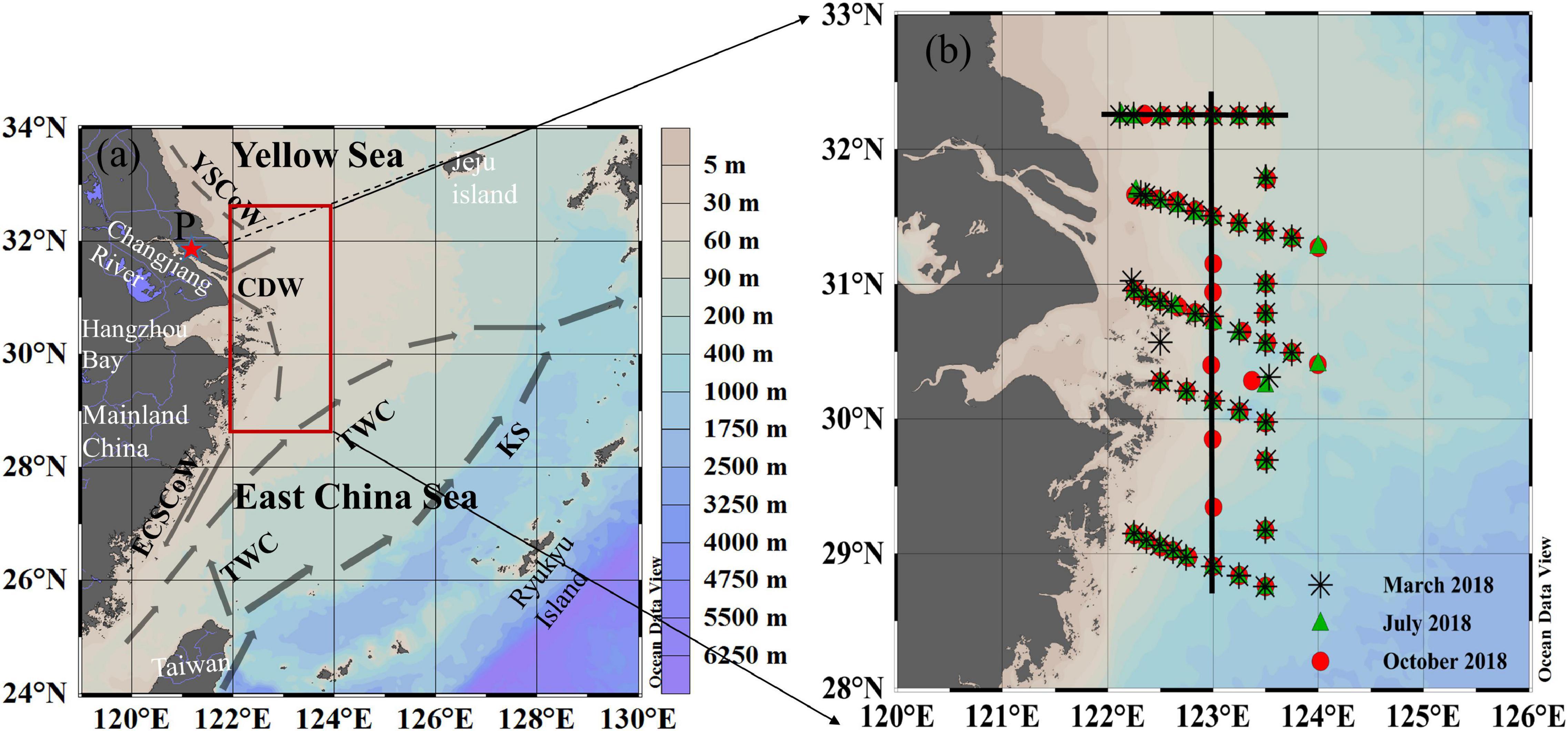
Figure 1. (a) Schematic map of the bathymetry and current system of the ECS, (b) maps of sampling stations in March, July, and October, 2018. In panel (a), the framed region indicates the area under study. The thin line from the northern corner of the Changjiang estuary to Jeju Island is the traditional boundary between the YS and the ECS. Dark gray arrow sketches major currents in the ECS (Chen, 2009), including the Kuroshio (KS), the Taiwan Warm Current (TWC), the East China Sea Coastal Water (ECSCoW), the Changjiang Diluted Water (CDW), and the Yellow Sea Coastal Water (YSCoW). The station P (red star, 121.10°E, 31.75°N) was used to represent the freshwater end-member for deriving the PO₄^3– hypothetical mixing line between the freshwater and seawater end-member of the CDW. The direct lines in (b) are transects 32°N and 123°E.

Sampling and Analytical Methods

The field investigations were carried out aboard the R/V Kexue 3 from March 9 to 19, July 11 to 20, and October 11 to 22, 2018. The sampling stations and cruise transects are shown in Figure 1b. The sampling and analytical methods for carbonate parameters strictly followed the recommended standard operating procedures described by Dickson et al. (2007) and the methods of Zhai et al. (2014a,b). For each station, water samples were collected at two or three depths using 12 L Niskin bottles mounted on a rosette assembly. Temperature and salinity were measured using a conductivity–temperature–depth (CTD) system (SBE 9/11-plus).

Samples of nutrients were first filtered with a 0.45 μm Whatman GF/F membrane and then stored in 250 mL high-density polyethylene (HDPE) bottles and stored at –20°C until chemical analysis. Nitrate (N), phosphate (PO₄^3–), and silicate (Si) were determined using a segmented flow analyzer (model: Skalar SANPLUS, Netherlands) with a precision <5% (Zhang et al., 2007); the detection limits were 0.14 μM for N, 0.06 μM for PO₄^3–, and 0.07 μM for Si.

The Chlorophyll a (Chl a) samples were collected 250 mL from Niskin bottles, first filtered through 300 μm meshes followed by 0.68 μm Whatman GF/F membranes, which were then folded rapidly within an aluminum foil and stored at –20 °C until analysis. Chl a on membranes was extracted using 90% acetone and then analyzed using a fluorescence spectrophotometer (Lengguang Tech F9700) based on the procedure described by Parsons et al. (1984).

A_T samples were stored in 250 mL HDPE bottles without filtering. The samples were poisoned with 100 μL saturated mercuric chloride (HgCl₂) solution and stored in a laboratory at 25°C. A_T was determined at 25°C by versatile instruments for the determination of titration alkalinity (VINDTA 3C) (Mintrop et al., 2000). Certified reference materials (CRM; Batch 156) from A. G. Dickson’s lab at the Scripps Institute of Oceanography were used for calibration and accuracy assessments of A_T measurements, and the accuracy and precision were determined to be higher than ± 2 μmol/kg.

Samples for pH_T were stored in 500 mL high-quality borosilicate glass bottles without filtering, poisoned with 200 μL saturated HgCl₂ solution, and stored at room temperature until measurement in the laboratory. pH_T was measured using an automated flow-through system for embedded spectrophotometry (Reggiani et al., 2016) with a precision of ±0.0005 pH unit. The indicator dye used was thymol blue (TB) sodium salt (TCI #FCP01, Tokyo Chemical Industry). Although Hudson-Heck and Byrne (2019) stated that “only low levels of impurities are typically present in off-the-shelf TB,” we evaluated the impurity of the indicator used following the approaches of Douglas and Byrne (2017) and Hudson-Heck and Byrne (2019) and identified that the pH_T correction was –0.00083. We measured the pH_T of CRM during the process of measuring the pH_T samples as a standard procedure. We calculated the CRM reference pH_T value at a temperature of 25°C using CO2SYS based on the salinity (33.455), C_T, A_T, PO₄^3–, and Si of CRM batch 156. The dissociation constants for H₂CO₃ were determined by Lueker et al. (2000), and the dissociation constant for HSO₄^– ions was determined by Dickson (1990). We measured the pH_T value of CRM at 25°C and salinity of 33.455 and compared it with the CRM reference pH_T (Supplementary Figure 1). The mean and standard deviation (SD) of the comparison were 0.0012 ± 0.0036 (n = 44) and 93% of residuals were within ± 0.006.

Calculation of Other Carbonate System Parameters

Total dissolved inorganic carbon (C_T) and pCO₂ were calculated using in situ temperature, salinity, PO₄^3–, Si, measured pH_T, and A_T using the CO2SYS.XLS (version 16) program developed by Pelletier et al. (2011), which is an updated version of CO2SYS.EXE (Lewis and Wallace, 1998). The dissociation constants for H₂CO₃ were determined by Lueker et al. (2000), and the dissociation constant for HSO₄^– ions was determined by Dickson (1990). In this study, we compared the carbonate properties obtained from the constants of Hansson (1973), Mehrbach et al. (1973), Dickson and Millero (1987), Lueker et al. (2000) and Millero et al. (2006) constants. We then found that, for our data range of temperature, salinity, pH_T, and A_T, the calculated pCO₂ difference was ∼3%. However, the carbonate parameters were calculated following Lueker et al. (2000) as recommended for best practices (Dickson et al., 2007). Thus, we chose the one for our calculations. Based on our measurements, uncertainties in pH_T and A_T measurements resulted in a calculated uncertainty of approximately ± 2 μatm in pCO₂.

CO₂ Flux Calculations

FCO₂ (mmol CO₂/m²/day) was calculated from:

$$FC{O}_2=k\times s\times \mathrm{△}pC{O}_2(1)$$

where k is the CO₂ transfer velocity (cm/h), s is the solubility of CO₂ in seawater (mol/kg) (Weiss, 1974), and ΔpCO₂ is the difference between the sea surface pCO₂ and the CO₂ concentration in the atmosphere. Atmospheric CO₂ concentrations were derived from the Tae-ahn Peninsula observation site (36.7376°N, 126.1328°E; Republic of Korea¹), after correction for water vapor pressure to 100% humidity with in situ temperature and salinity data (Weiss and Price, 1980). A positive flux indicates the release of CO₂ from the ocean to the atmosphere. The gas transfer velocity is a function of wind speed. However, as there is currently no universally accepted relationship, we compared the relationships between k and wind speed proposed by Nightingale et al. (2000) (hereafter referred to as N00), Ho et al. (2006) (H06), and Wanninkhof et al. (2009) (W09) to estimate FCO₂ in this study. The reason is that the N00 and H06 used the dual-deliberate tracer methods of ³He and SF₆ to obtain direct estimates of k, and the experiments by N00 were performed in coastal seas, while the latter was performed in the Southern Ocean. However, W09 proposed using the nonzero intercepts for accounting for zero wind speed gust environments or zero wind-driven processes and utilizing the global bomb ¹⁴C constraint and information from the literature to determine k.

$$\mathrm{N00}\mathit{\hspace{1em}\hspace{1em} }k=\left(0.333\times u+0.222\times u^2\right)\times {(Sc/660)}^{-0.5}(2)$$

$$\mathrm{H06}\mathit{\hspace{1em}\hspace{1em} }k=0.266\times u^2\times {(Sc/660)}^{-0.5}(3)$$

$$\mathrm{W09}\mathit{\hspace{1em}\hspace{1em} }k=\left(3+0.1\times u+0.064\times u^2+0.011\times u^3\right)\times {(Sc/660)}^{-0.5}(4)$$

where u is the daily wind speed at a height of 10 m (in m/s). We used the daily average wind speed from CCMP Version–2.1 analyses produced by Remote Sensing Systems with a spatial resolution of 0.25° × 0.25° grids.² Sc is the Schmidt number for CO₂ in seawater computed from in situ temperature data (Wanninkhof, 2014).

Results

Classification of Water Types

In our study, the surface waters were grouped into three types, namely, (1) YSW, (2) CDW, and (3) ECSSW, according to the classification described by Chou et al. (2009), Qi et al. (2014), and Zhai et al. (2014a) (T–S diagram, Figure 2). The temperature and salinity variations of the three water types are listed in Supplementary Table 1. The locations of the various water types in the three surveys (Figure 3) were generally consistent with the known distribution pattern in the ECS (Figure 1a). The YSW was classified under the northeast part of our study area in March and October, whereas the CDW was identified outside the Changjiang River estuary, where the water depth was <50 m. The remaining area was identified as ECSSW (Figure 3).

FIGURE 2

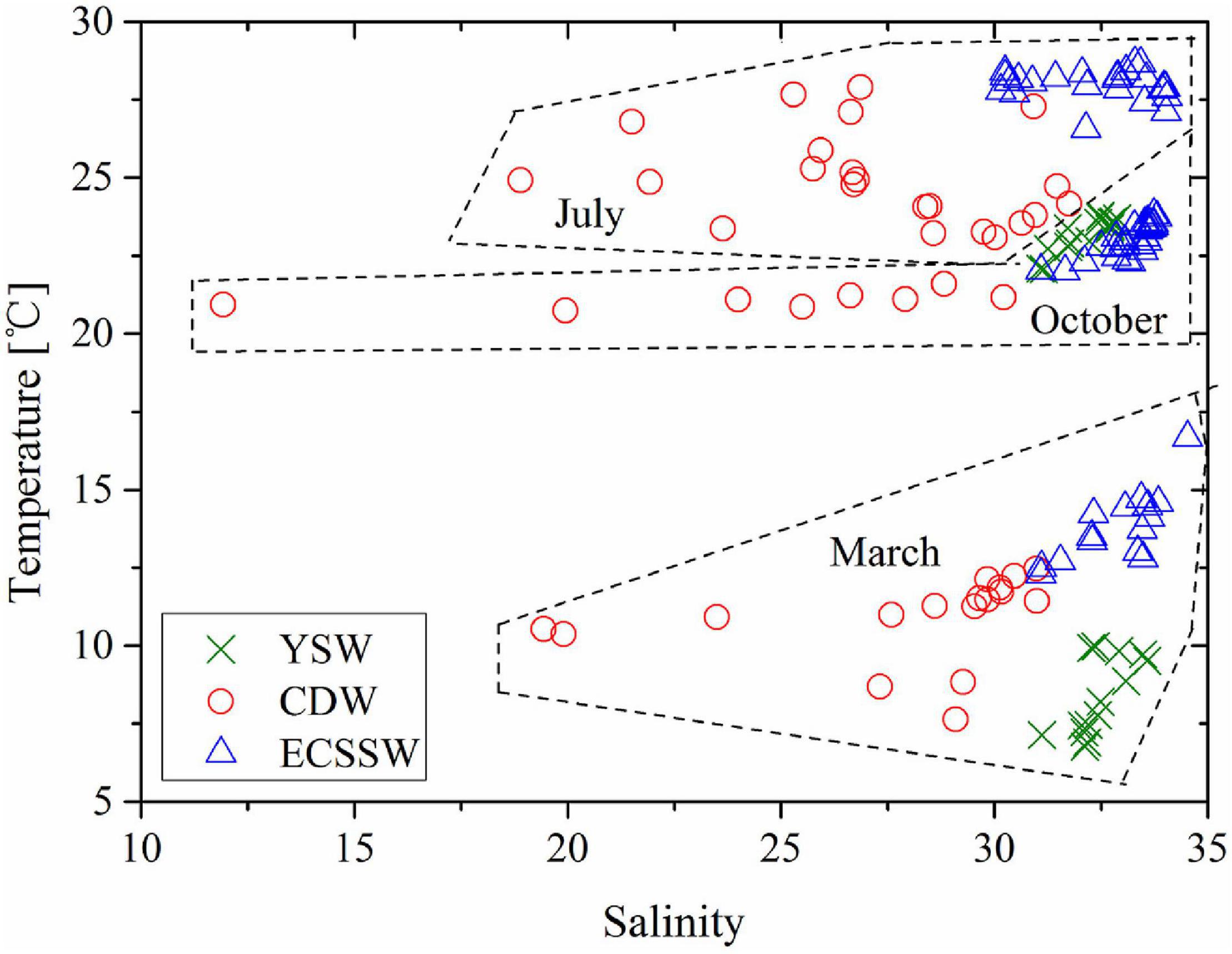
Figure 2. Temperature versus salinity plot for surface water of the study area in March, July, and October, 2018, for three water masses: Yellow Sea Water (YSW), Changjiang Diluted Water (CDW), and East China Sea Shelf Water (ECSSW). Dashed boxes show separate water masses in different seasons.

FIGURE 3

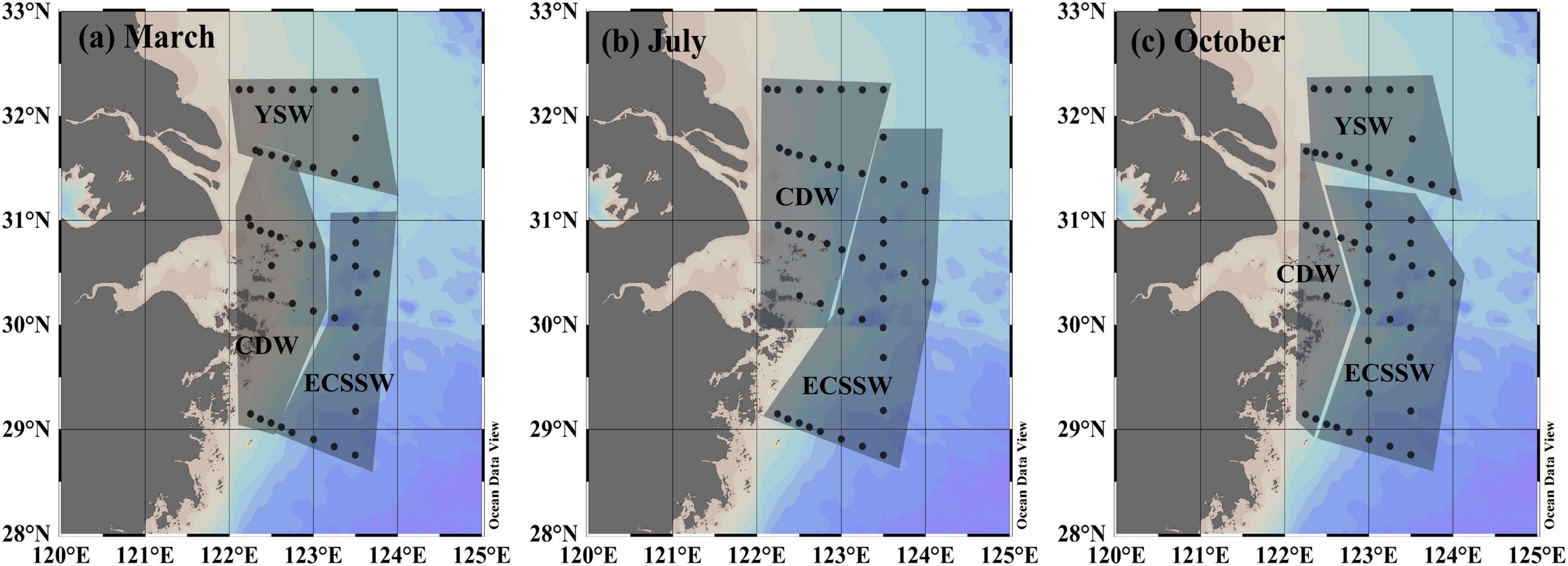
Figure 3. Geographic positions of the three water types in the outer Changjiang estuary in (a) March, (b) July, and (c) October.

Distribution of Hydrological and Carbonate Parameters in Various Water Types

The surface distributions of temperature, salinity, pH_T, A_T, C_T, and pCO₂ in March, July, and October are presented in Supplementary Figure 2. Their range, average, and SD values for the three different water types are summarized in Supplementary Table 1. The distributions of these parameters not only have significant seasonal variations but also vary between different water masses.

The distributions of temperature and salinity are consistent with the circulation systems and hydrological environments of the ECS (Lee and Chao, 2003). In our three surveys, the intermediate salinity (31.11–33.57 in March and 31.08–32.87 in October) was limited in the YSW, while higher temperatures and salinity (12.28–16.67°C and 31.09–34.52; 26.56–28.66°C and 30.15–34.04; 22.00–23.81°C and 31.09–33.80 in March, July, and October, respectively) were observed in the ECSSW as a result of the high temperature and salinity of the Taiwan Warm Current (TWC). Low salinities (< 31) occurred in the CDW (19.44–31.00, 18.89–31.75, and 11.93–30.22 in March, July, and October, respectively) with low temperatures in July (23.08–27.90°C) and October (20.74–21.60°C) (Supplementary Figures 2A,B).

Generally, the CDW had the lowest pH_T (pH_T < 8). Intermediate pH_T values were mainly detected in the YSW area (8.042–8.104 in March and 7.927–8.008 in October), while a relatively high pH_T was found in the ECSSW area (8.078–8.117 in March and 7.938–8.085 in October). However, in summer, the highest pH_T (8.420) and the lowest pH_T (7.729) values occurred in the CDW area, the highest value may be the result of net biological production, and the lowest was due to biological respiration and the decomposition of organic matter (Supplementary Figure 2C).

Similar to the distribution of pH_T, low A_T values always occurred in the CDW (2168–2317, 2069–2232, and 1982–2281 μmol kg^–1 in March, July, and October, respectively). In March and October, a high A_T was found in the YSW (2263–2356 and 2227–2282 μmol/kg in March and October, respectively), while the ECSSW had intermediate A_T values (2246–2273 and 2229–2248 μmol/kg in March and October, respectively) (Supplementary Figure 2D). The high A_T in YSW may result from Huanghe River discharge with high A_T concentrations (2874–3665 μmol/kg) (Chen et al., 2005) due to intensive carbonate weathering and erosion in the drainage basin (Zhang et al., 1990).

High concentrations of C_T were found in the YSW in March (2071–2205 μmol/kg) and October (1987–2082 μmol/kg). In July, a large C_T range was observed in the CDW (1675–2070 μmol/kg). Low concentrations of C_T were found in the ECSSW during the three surveys, with ranges of 2020–2061, 1786–1958, and 1941–2040 μmol/kg in March, July, and October, respectively (Supplementary Figure 2E).

Surface pCO₂ shared a similar yet inverse distribution to pH_T, (Supplementary Figures 2C,F). A low pH_T and high pCO₂ were observed in the CDW (357–554 and 506–719 μatm in March and October, respectively). This was caused by the biological decomposition of organic materials imported by the Changjiang River discharge, which produced a large amount of CO₂. A low pCO₂ was seen in the YSW (344–416 and 438–561 μatm in March and October, respectively), while the lowest pCO₂ was found in the ECSSW (330–369 and 350–537 μatm in March and October, respectively). However, the CDW area exhibited a very large pCO₂ range (136–965 μatm) in July.

Air–Sea CO₂ Flux

Figure 4 shows the surface distributions of ΔpCO₂ (pCO_{2, sea} – pCO_{2, air}) and FCO₂ (calculated after N00, H06, and W09 described in Section “CO₂ flux calculations”) in the three surveys. Table 1 summarizes the FCO₂ values for each water mass and the entire study area. Overall, the distribution patterns of ΔpCO₂ and FCO₂ were consistent with pCO₂ (Figure 4 and Supplementary Figure 2F), and clear seasonal variations in FCO₂ were observed. In March, the pCO₂ of the entire study area was lower than the atmospheric CO₂ concentration, while in July and October, it was the opposite (Table 1). However, the pCO₂ near the Changjiang River estuary was independent of the seasons, and was always higher than the atmospheric CO₂ concentration and acted as a CO₂ source (Figure 4). For the three water types, ΔpCO₂ < 0 in March, ΔpCO₂ > 0 in October; in July, ΔpCO₂ > 0 in the CDW and ΔpCO₂ < 0 in the ECSSW (Table 1).

FIGURE 4

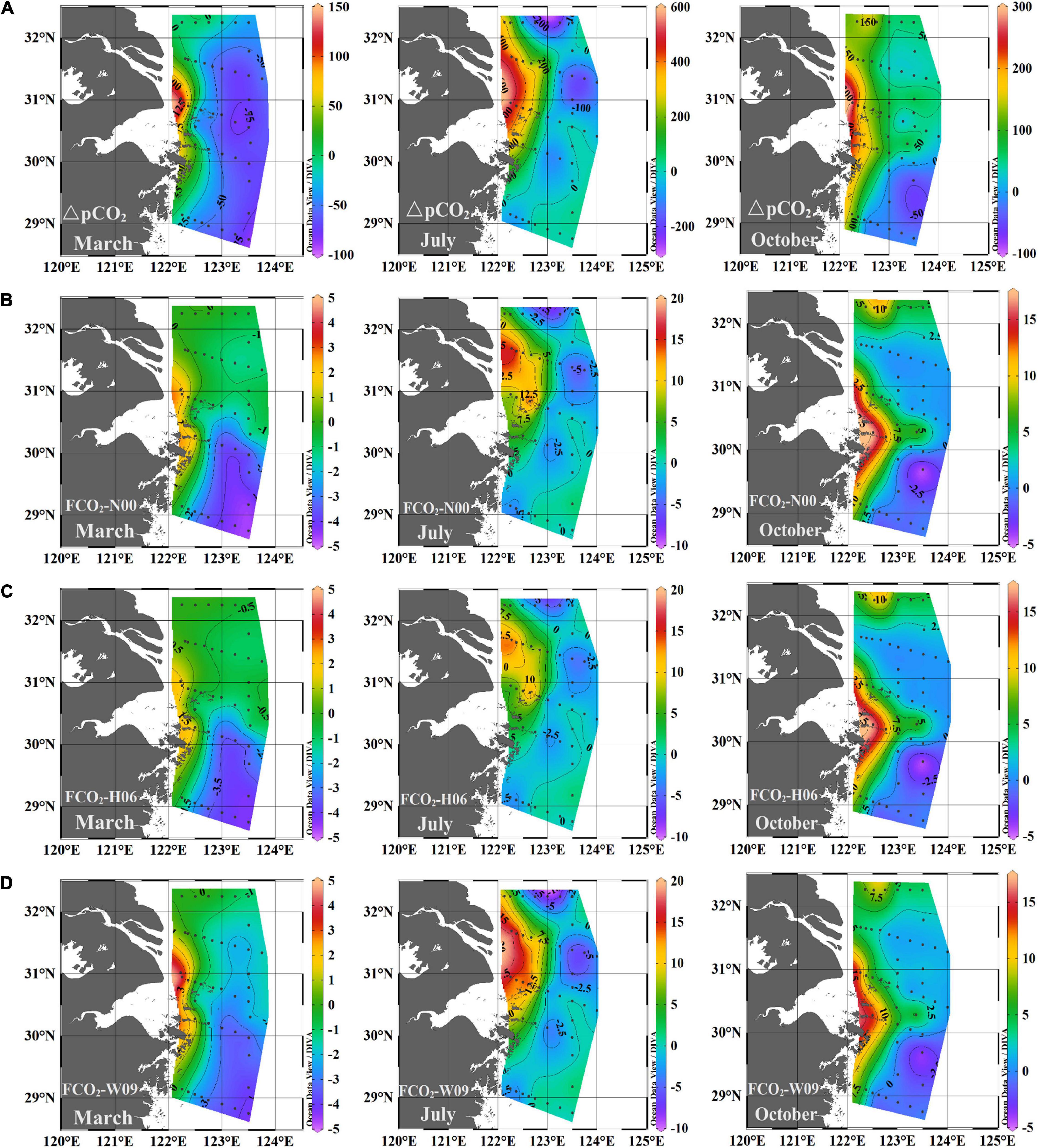
Figure 4. Spatial distribution of (A)ΔpCO₂ and FCO₂ (B, C, D) calculated using the respective k-wind speed relationships of N00, H06, and W09 in March, July, and October, 2018.

TABLE 1

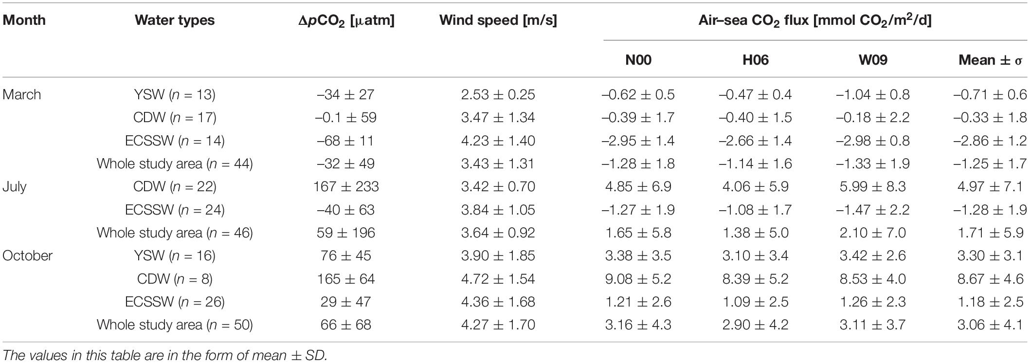
Table 1. Surface water average ΔpCO₂ (μatm) and FCO₂ (mmol CO₂/m²/day) using three different gas transfer velocity (k) formulas for the water types in March, July, and October, 2018.

The FCO₂ calculated by N00, H06, and W09 showed similar spatial distributions (Figures 4B–D), and the FCO₂ values calculated for the entire study area were also similar (Table 1). However, for each water mass, the FCO₂ calculated by W09 was different from those calculated using the other two formulas, especially for the CDW and YSW. For W09, the constant term dominated at low wind speeds, and the k value calculated by W09 was much higher than the others. The wind speed was relatively low (<4 m/s), especially in spring and summer. Therefore, the FCO₂ calculated by W09 was much higher than that obtained from the other two formulas (Table 1). Overall, the study area was a CO₂ sink in March and a CO₂ source to the atmosphere in July and October. The average FCO₂ was –1.25 ± 1.7, 1.71 ± 5.9, and 3.06 ± 4.1 mmol CO₂/m²/day, respectively (Table 1). According to the average FCO₂ calculated by the three gas exchange formulas, the water type acts as a source or sink of CO₂, which may change with the seasons (Figure 5). The YSW and ECSSW were net CO₂ sinks in March and July (–0.71 ± 0.6 mmol CO₂/m²/day in the YSW and –2.86 ± 1.2, –1.28 ± 1.9 mmol CO₂/m²/day in the ECSSW) and transformed to net sources by October (3.30 ± 3.1 mmol CO₂/m²/day in the YSW and 1.18 ± 2.5 mmol CO₂/m²/day in the ECSSW). The CDW was a net CO₂ sink in March and a net CO₂ source in July and October (–0.33 ± 1.8, 4.97 ± 7.1, and 8.67 ± 4.6 mmol CO₂/m²/day in March, July, and October, respectively).

FIGURE 5

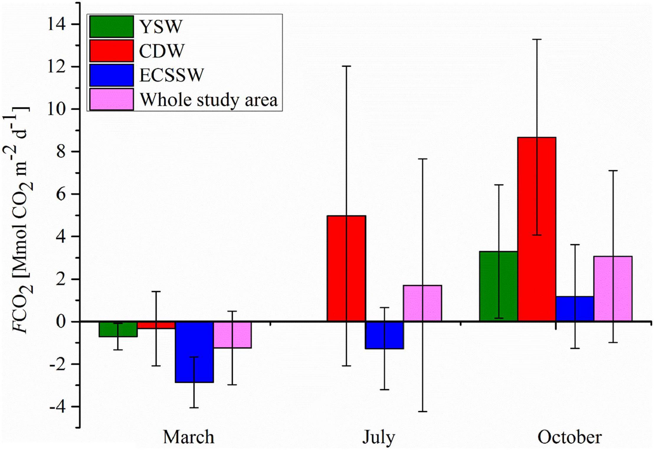
Figure 5. Air–sea CO₂ fluxes in the different water types in March, July, and October, 2018. The FCO₂ in this figure were the average values calculated by the three gas exchange formulas mentioned in Section “CO₂ flux calculations.”

Water Mixing Behavior of the Surface Water Carbonate System

A_T is considered a quasi-conservative carbonate parameter, and its relationship with salinity can indicate water mixing behavior (Zhai et al., 2014a,b). Figure 6 shows that they were found significant correlations between the A_T and salinity of the three water types in March, July, and October. The lowest A_T and salinity were detected in the CDW, while the YSW had the highest A_T values.

FIGURE 6

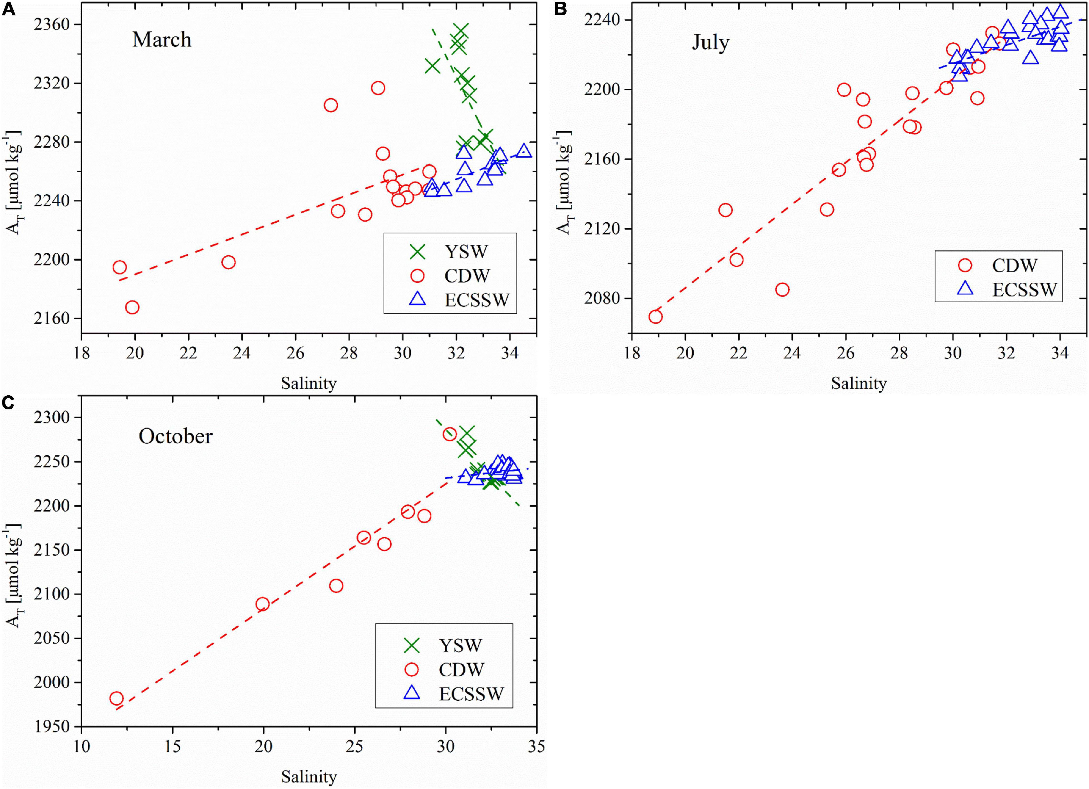
Figure 6. A_T versus salinity in (A) March, (B) July, and (C) October of the study area using the same water type definitions as in Figure 2. Dashed lines represent the regression lines for each water type.

In the YSW, there was a negative relationship between A_T and salinity in March and October [Eqs. (5) and (6), Figures 6A,C].

$$A_T^{YSW}=-36.41\times Salinity+3489.40$$

$$(\mathrm{March},\mathrm{n}=13,\mathrm{r}=-0.727,\mathit{P}<0.01)(5)$$

$$A_T^{YSW}=-21.40\times Salinity+2928.33$$

$$(\mathrm{October},\mathrm{n}=16,\mathrm{r}=-0.833,\mathit{P}<0.01)(6)$$

If Eqs. (5) and (6) were extrapolated to the average salinity of the ECSSW in March (32.80) and October (33.16), the calculated A_T values were 2295.15 and 2218.71 μmol/kg in March and October, respectively. These values are very close to the average A_T values of the ECSSW in March and October (Supplementary Table 1). This result suggests water mixing between the YSW and ECSSW in March and October.

In the CDW and ECSSW, A_T–salinity had positive relationships in March, July, and October (Eqs. (7)–(12), Figure 6):

$$A_T^{CDW}=6.79\times Salinity+2054.12$$

$$(\mathrm{March},\mathrm{n}=17,\mathrm{r}=0.676,\mathit{P}<0.01)(7)$$

$$A_T^{ECSSW}=7.37\times Salinity+2018.78$$

$$(\mathrm{March},\mathrm{n}=14,\mathrm{r}=0.791,\mathit{P}<0.01)(8)$$

$$A_T^{CDW}=12.01\times Salinity+1845.90$$

$$(\mathrm{July},\mathrm{n}=22,\mathrm{r}=0.912,\mathit{P}<0.01)(9)$$

$$A_T^{ECSSW}=5.26\times Salinity+2057.30$$

$$(\mathrm{July},\mathrm{n}=24,\mathrm{r}=0.757,\mathit{P}<0.01)(10)$$

$$A_T^{CDW}=14.14\times Salinity+1800.78$$

$$(\mathrm{October},\mathrm{n}=8,\mathrm{r}=0.955,\mathit{P}<0.01)(11)$$

$$A_T^{ECSSW}=2.30\times Salinity+2162.64$$

$$(\mathrm{October},\mathrm{n}=26,\mathrm{r}=0.312,\mathit{P}=0.12)(12)$$

There was no significant correlation between the salinity and A_T in the ECSSW in October [Eq. (12)]. The Changjiang river end-member has an A_T of 1711–1831 μmol/kg in spring, 1630–1950 μmol/kg in summer (Zhai et al., 2007), and 1712–1781 μmol/kg in autumn (Xiong et al., 2019). If Eqs. (7), (9), and (11) were extrapolated to the freshwater end-member (salinity = 0), the intercept of A_T was 2054.12, 1845.90, and 1800.78 μmol/kg. The value in March is much higher than the reported A_T range (Zhai et al., 2007), possibly owing to the CDW mixing with high A_T YSW. If Eqs. (7), (9), and (11) extrapolated to the ECSSW average salinity (32.80 in March, 32.34 in July, and 33.16 in October), the calculated A_T results were 2276.83, 2234.30, and 2269.66 μmol/kg, respectively, which were very close to the observed average A_T values of the ECSSW (Supplementary Table 1). This indicates mixing between the CDW and ECSSW during the three surveys. The A_T range of the Kuroshio (KS) and TWC surface water was 2300–2310 μmol/kg at a salinity of 35 (Chen and Wang, 1999). Extrapolating to salinity = 35, the A_T values were 2291.77, 2276.73, and 2295.68 μmol/kg using Eqs. (7), (8), and (11), respectively, which were close to the range of KS and TWC surface water. Thus, the ECS offshore end-member was dominated by TWC surface water, agreeing with the results obtained by Chen et al. (1995).

Discussion

Processes Controlling the Seasonal Variation of Sea Surface Water pCO₂

Compared with the changes in the concentration of CO₂ in the atmosphere, pCO₂ varies greatly and ultimately determines the spatial and seasonal variabilities in ΔpCO₂ (Luo et al., 2015). Surface temperature and salinity-driven CO₂ solubility, water mixing, and biological processes control the temporal and spatial variabilities of sea surface pCO₂ (Wang et al., 2013). Considering the complex relationships between environmental drivers [i.e., temperature (T), salinity (S), and Chl a], and pCO₂ variation, a Pearson correlation analysis was conducted to evaluate the potential drivers of pCO₂ (Table 2). In the following sections, the drivers shaping the pCO₂ variability in different water masses are discussed.

TABLE 2

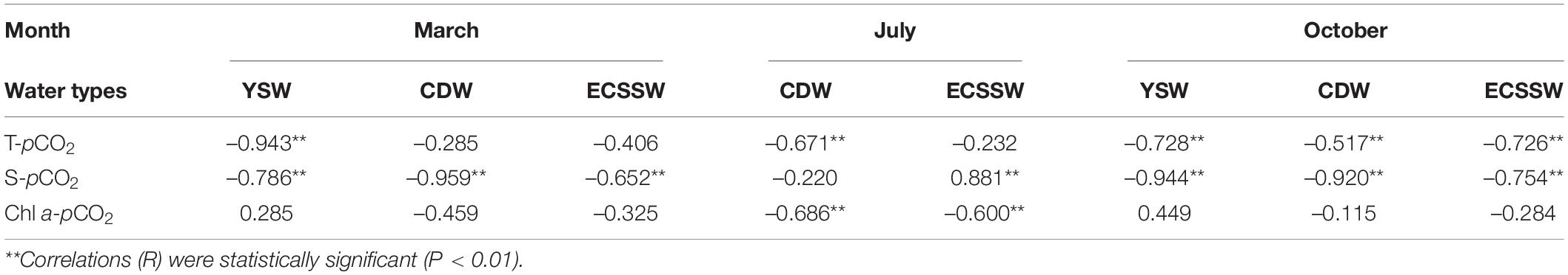
Table 2. Pearson correlations of pCO₂ and potential drivers (T, S, and Chl a) in March, July, and October.

Relationship Between Temperature and pCO₂

Thermodynamically, pCO₂ increases exponentially with increasing temperature and follows the empirical formula of Takahashi et al. (1993):

$$\partial lnpC{O}_2/\partial T={0.0423}^{°}{C}^{-1},(13)$$

Yet, pCO₂ and the temperature of the water masses in March, July, and October showed significant negative correlations (Figures 7A–C and Table 2), indicating that temperature was not the dominant factor in regulating pCO₂ variation. Similarly, a negative relationship between pCO₂ and the surface water temperature was also observed in the vertically well-mixed ECS shelf in winter (Chou et al., 2011) and the offshore area of the South Yellow Sea in winter and summer (Zhang et al., 2010). There are two major reasons for the negative relationship between pCO₂ and temperature: the first is that vertical mixing transported the CO₂-rich bottom water to the surface (Chen et al., 2007), and the second is that the intensive biological activity uptake of CO₂ dominates over the temperature effect on pCO₂ (Zhang et al., 2010) (see Section “Influences of biological processes on pCO₂ variability”). Mixing of coastal water (cold and rich in CO₂) and offshore water (warm and has lower pCO₂) is considered as the main controlling process in March and October (Supplementary Figures 2A,F).

FIGURE 7

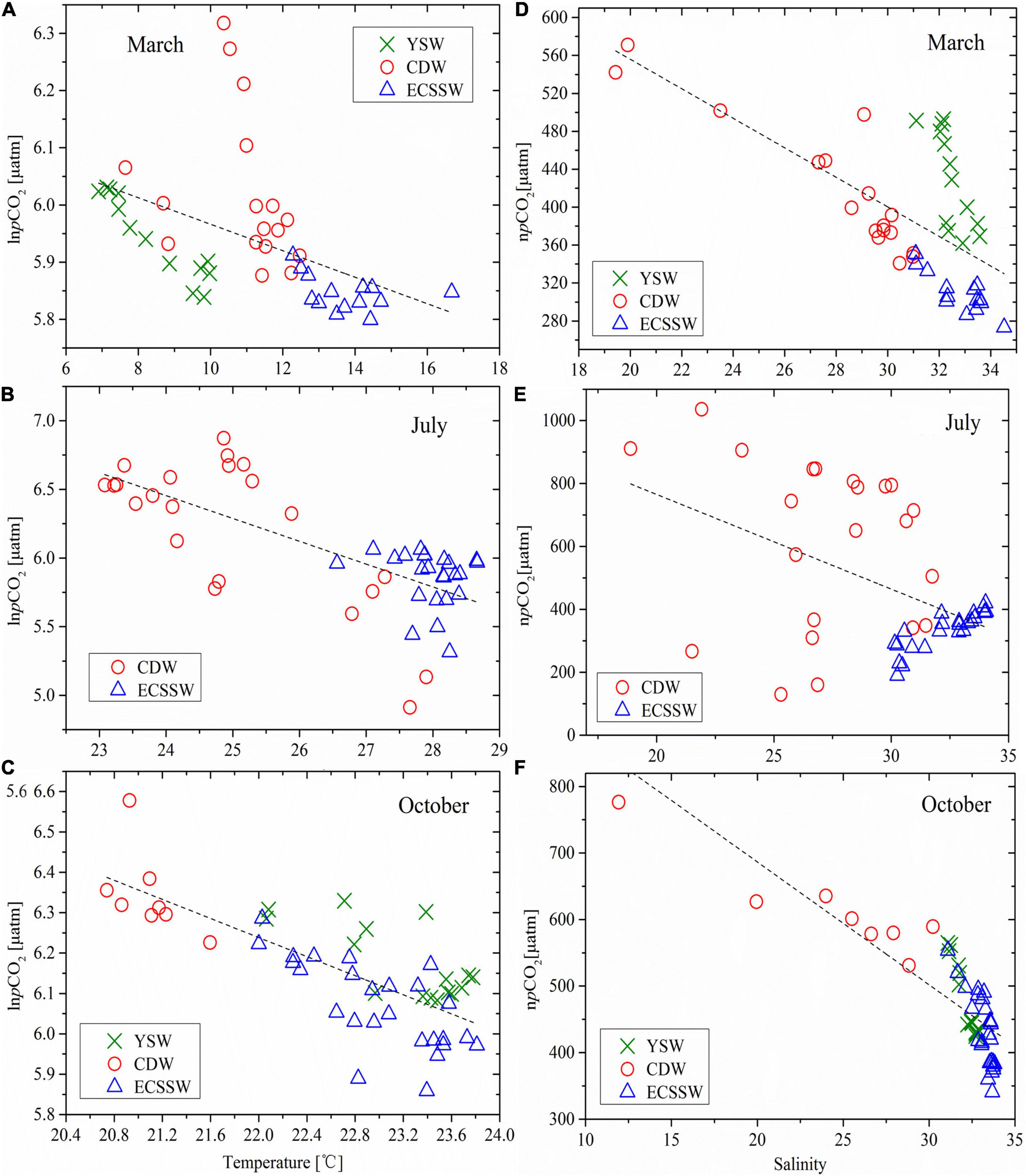
Figure 7. (A–C) lnpCO₂ versus temperature and (D–F) npCO₂ versus salinity in March, July, and October, with the same water type zonings as Figure 2. npCO₂ was normalized to the average temperature of 11.07°C in March, 26.55 °C in July, and 22.75°C in October. Dashed lines are the regression lines of lnpCO₂/npCO₂ with all data.

Effects of Water Mixing Processes on pCO₂ Variability

To remove the influence of temperature, pCO₂ was first normalized npCO₂ = pCO₂ × exp[0.0423 × (T_mean – T)] [Eq. (13)] to the average temperatures of 11.07°C, 26.55°C, and 22.75°C in March, July, and October, respectively. Figures 7D–F presents the relationships between npCO₂ and salinity in the three different seasons. There were negative correlations between npCO₂ and salinity in March (r = –0.673, P < 0.01), July (r = –0.469, P < 0.01), and October (r = –0.845, P < 0.01). This suggests that pCO₂ was dominated mainly by mixing between high salinity/low pCO₂ offshore ECSSW and low salinity/high pCO₂ nearshore CDW, which is consistent with the results of Zhai and Dai (2009). Considering the relationship between npCO₂ and salinity in each water mass, it must be highlighted that there were strong negative correlations in all three water masses in March and October. Furthermore, there was a significant positive correlation in the ECSSW (r = 0.869, P < 0.01) and no evident relationship in the CDW (r = –0.171, P = 0.445) in July (Figure 7E), which was probably caused by non-physical (i.e., metabolic) processes (Zhai and Dai, 2009).

In March, cooling resulted in the lowest pCO₂ measured in 2018, which was also shown to be a major driver of CO₂ sink (Tsunogai et al., 1999). However, the YSW and ECSSW had the highest average pCO₂ level in October (Supplementary Table 1) and was the atmospheric CO₂ source (Figure 5). The significant positive relationship between npCO₂ (normalized to the average temperature of 22.75°C of October) and NC_T (salinity normalized C_T, NC_T = C_T × 35/S, r = 0.939, P < 0.01) (Figure 8) indicated that the C_T-enriched bottom water was mixed with the surface, resulting in high surface pCO₂ (Zhai and Dai, 2009; Zhang et al., 2010; Guo et al., 2015). The vertical distributions of temperature and salinity along the transects of 32°N (in the YSW) and 123°E (in the ECSSW) (Figure 9) indicated that deep vertical mixing occurred in October. Consequently, the YSW and ECSSW were CO₂ sources in October.

FIGURE 8

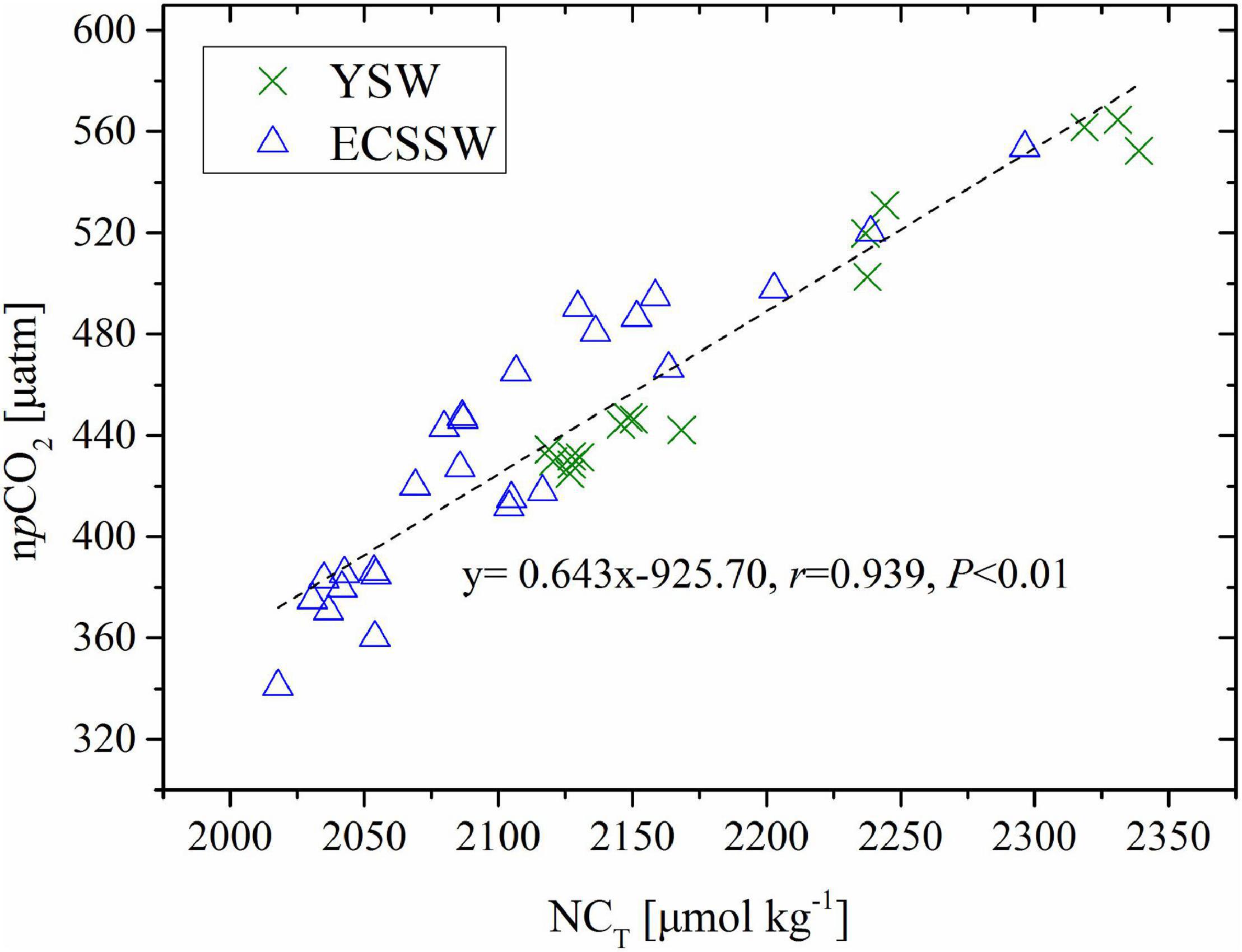
Figure 8. Correlation of surface pCO₂ normalized to the average temperature of 22.75°C in October (npCO₂) and salinity normalized C_T (NC_T).

FIGURE 9

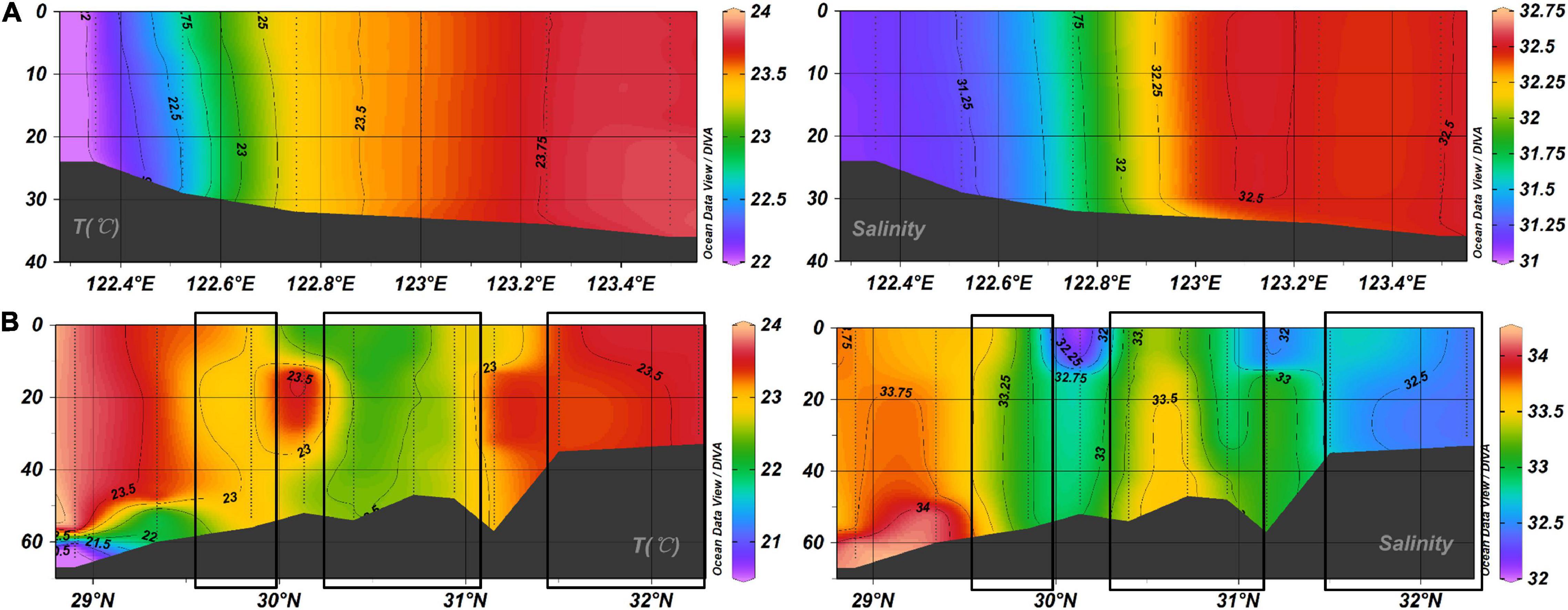
Figure 9. Vertical distributions of temperature and salinity along (A) 32°N, (B) 123°E in October 2018. The boxes in (B) represent the vertical water mixing.

Influences of Biological Processes on pCO₂ Variability

The highest phytoplankton concentrations were found in spring and summer in the ECS, enabled by abundant nutrients and suitable temperatures (Guo et al., 2015; Qu et al., 2017). Although not an optimum indicator of biological production, the level of Chl a is often used to indicate phytoplankton biomass. During the three surveys, summer was the only season with a significant relationship between pCO₂ and Chl a (Table 2). The negative correlations between npCO₂ and Chl a in the CDW (r = –0.675, P < 0.01) and ECSSW (r = –0.556, P < 0.01) (Figure 10) indicated that biological production played an important role in pCO₂ drawdown. In July, phytoplankton uptake CO₂ in the surface water through photosynthesis and transport it to the deeper water through the biological pump, resulting in a corresponding decrease in surface pCO₂ and an increase in atmospheric CO₂ uptake. As a result, the ECSSW was a net CO₂ sink in July. However, the CDW acted as a CO₂ source although the biological production promoted the drawdown of surface pCO₂, which may be attributed to the Changjiang River discharge, the details were discussed in Section “Potential effects of Changjiang River discharge.”

FIGURE 10

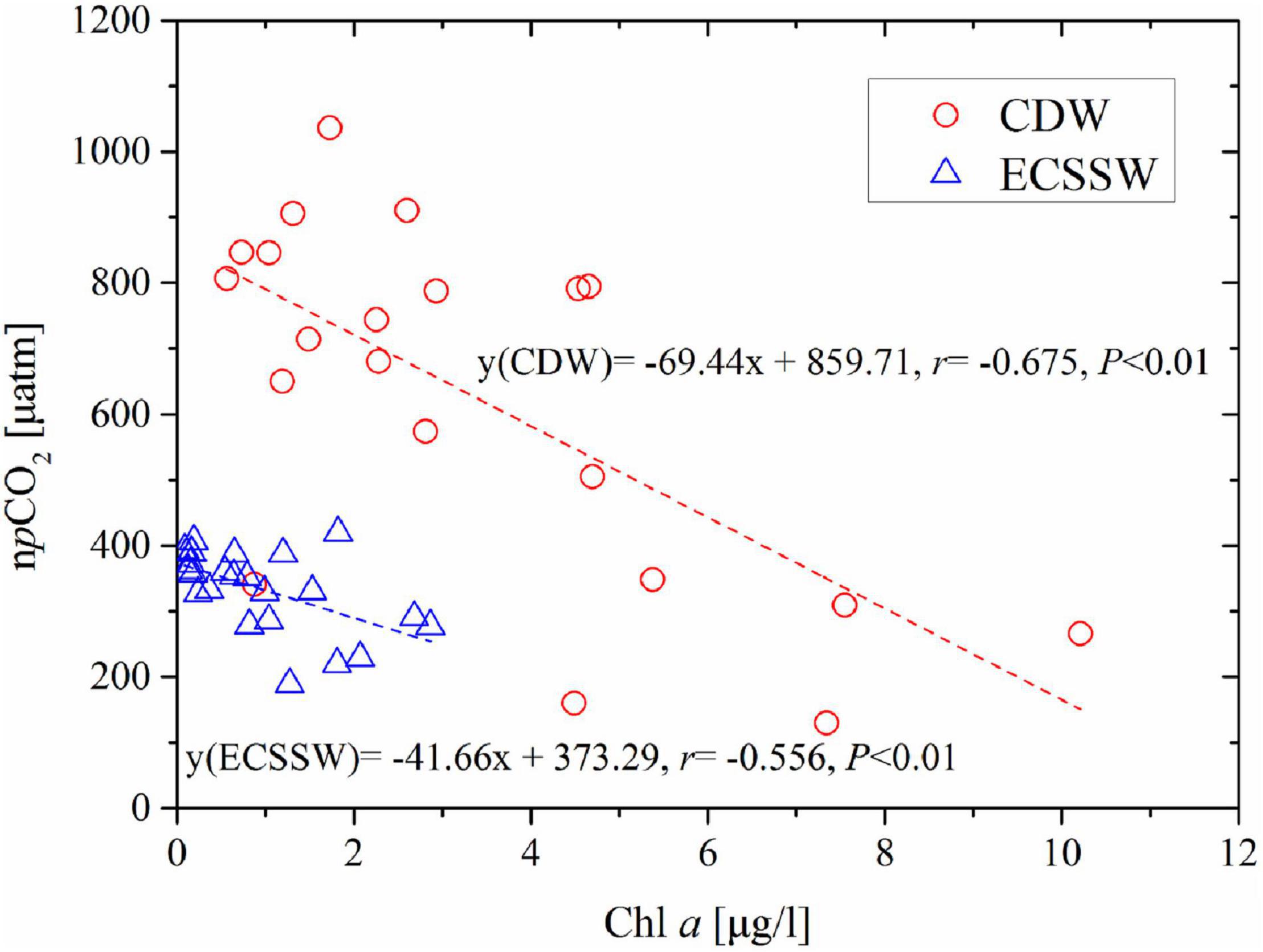
Figure 10. Correlations of temperature-normalized pCO₂ (npCO₂) and Chl a of YSW and ECSSW in July. The npCO₂ was normalized to an average temperature of 26.55°C.

Potential Effects of Changjiang River Discharge

The CDW region is significantly affected by Changjiang River inputs (Figure 11) and is a major determinant of CO₂ fluxes in the ECS shelf (Tseng et al., 2011). The CO₂ sink or source status in the CDW area mainly depends on the balance of CO₂ between the contributions from the Changjiang River discharge and the consumption of biological processes (Qu et al., 2017). Here, we adopted the method of Dai et al. (2013) to analyze why the CDW was a CO₂ source in July and October, especially in the summer, although biologically activity was high. According to Section “Water mixing behavior of the surface water carbonate system,” the surface water in the CDW is a two-end member mixing between freshwater and a seawater end-member originating from the TWC surface water. Figure 12A shows A_T as a conservative parameter that agrees with the predicted values and confirms the two end-members mixing in the surface water of the CDW. C_T is a non-conservative parameter that responds to biological activity. Thus, both C_T and PO₄^3– showed significant deviations from the predicted values (Figures 12B,C) below the hypothetical mixing line indicating biological removal.

FIGURE 11

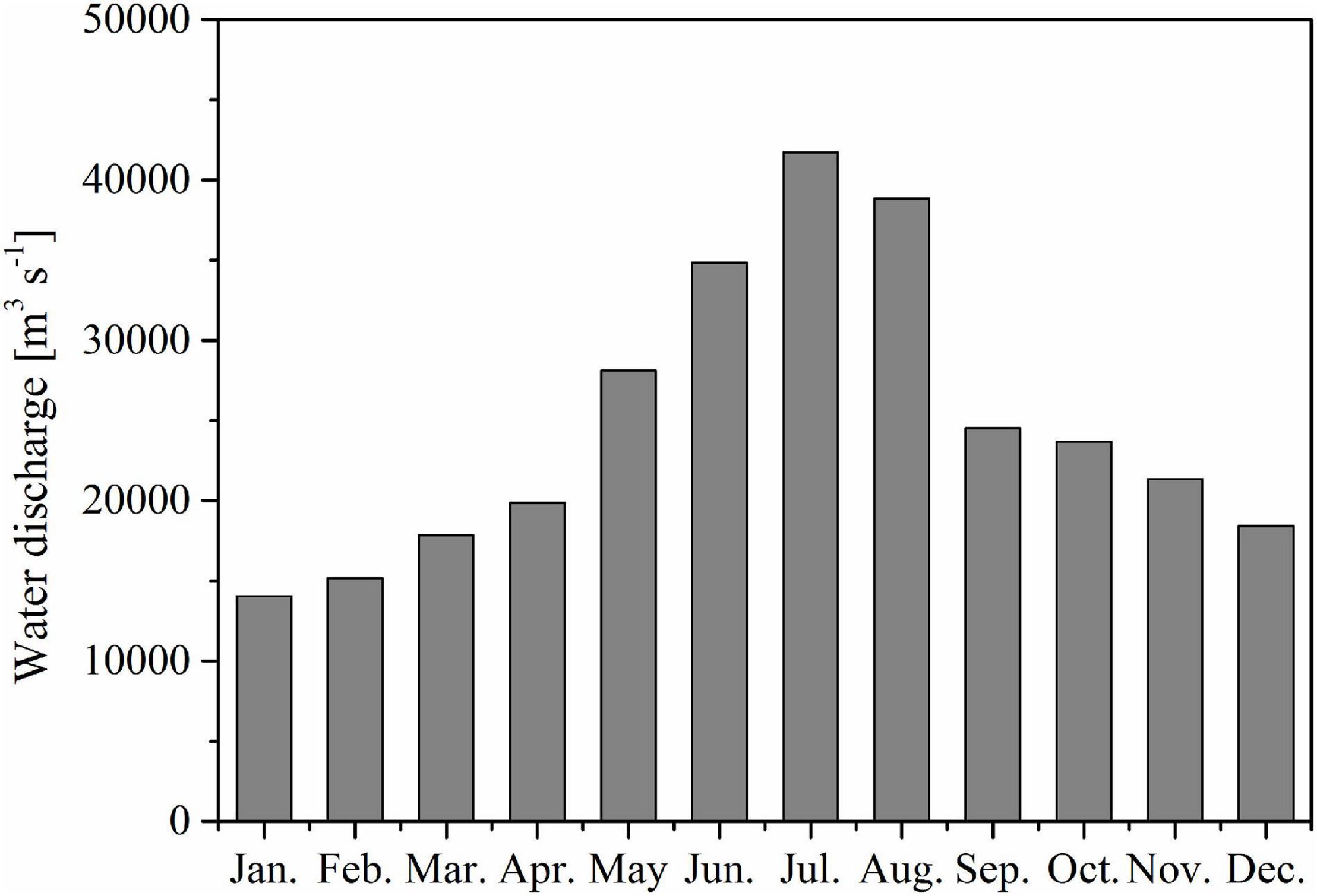
Figure 11. Monthly water discharge from Changjiang River in 2018 (Datong station, data derived from the China Bureau of Hydrology, http://www.mwr.gov.cn/).

FIGURE 12

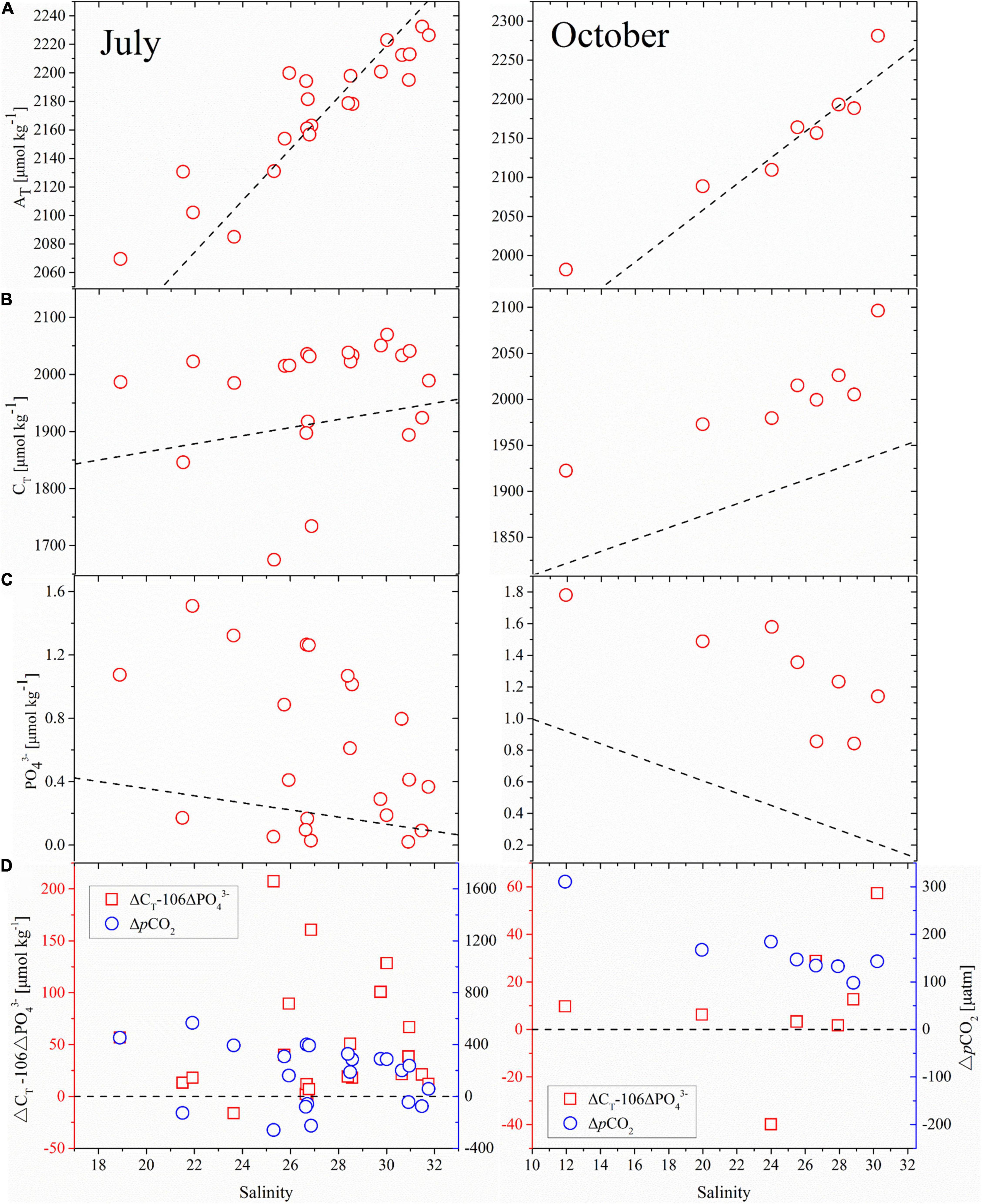
Figure 12. (A) A_T, (B) C_T, (C) PO₄^3–, and (D) ΔC_T –106ΔPO₄^3– (red squares) and ΔpCO₂ (blue circles) versus salinity in the surface water of CDW in July and October, 2018. The dashed lines in panels a-c represent the hypothetical mixing line between surface freshwater end-member and seawater end-member, in which A_T, C_T, and PO₄^3– are 1676, 1722, and 0.805 μmol/kg in July and 1724, 1744, and 1.385 μmol/kg in October in the freshwater end-member, respectively, and 2310 (Chen and Wang, 1999), 1971 (Chou et al., 2017), and 0.02 μmol/kg (Chen and Wang, 1999) in the seawater end-member, respectively. The A_T and C_T values of the freshwater end-member were obtained from Xiong et al. (2019) and the PO₄^3– values from station P (121.10°E, 31.75°N; Figure 1a), and the station samples were collected aboard the R/V Chuangxin 2 on July 17 and October 16, 2018. The dashed line in panel d represents the pCO₂ equilibrium between the seawater and the atmosphere.

Based on the method of Dai et al. (2013), ΔC_T and ΔPO₄^3– refer to the non-conservative portion of C_T and PO₄^3– in the surface water of CDW. Furthermore, the coupling of C_T and nutrient dynamics can be considered to follow the classic Redfield ratio (C: N: P = 106:16:1) (Redfield et al., 1963). When ΔC_T exceeds the corresponding 106ΔPO₄^3–, this can only be removed by CO₂ degassing into the atmosphere. In contrast, when ΔC_T is lower than the corresponding 106ΔPO₄^3–, this “deficient ΔC_T” can be compensated by atmospheric CO₂ uptake into the ocean. From Figure 12D, the apparent differences between ΔC_T and 106ΔPO₄^3– were, generally, above zero; indicating extra C_T accumulation in the surface water, driving the high pCO₂, and for CDW to be a CO₂ source in July and October (Figure 5). Therefore, in the CDW, the CO₂ produced by the decomposition and mineralization of terrestrial organic materials had exceeded the net CO₂ consumption of biological activities (Chen et al., 2008). The turbidity maximum zone (TMZ) is characterized by a high suspended particulate matter (SPM) concentration (Shen et al., 2020). The CDW area is very close to the TMZ in the three surveys, and Shen et al. (2020) found that a high SPM was consistent with the moving direction of the CDW. High SPM results in high turbidity and low transparency in the CDW, which is generally not optimal for phytoplankton growth and photosynthesis (Qu et al., 2017).

Seasonality in the Air–Sea CO₂ Flux

The magnitude of FCO₂ is determined by the wind speed, T- and S-driven solubility of CO₂, and ΔpCO₂. The seasonal atmospheric CO₂ sink and source pattern are determined by ΔpCO₂, and the wind speed affects the potential strength of CO₂ absorption or release (Luo et al., 2015). A Gray relational analysis was conducted to discuss the seasonal pattern of FCO₂ in different water types and its controlling factors (Supplementary Table 2). For the entire study area, the most influential factor for FCO₂ was ΔpCO₂ in July and October, whereas in March, wind speed, T, S, and ΔpCO₂ had similar controls on FCO₂. However, for each of the water types, the controls on FCO₂ were more complicated. In March, the most significant controlling factor of FCO₂ was ΔpCO₂ in the YSW. ΔpCO₂ was the least influential factor in the CDW and the ECSSW. In July, the most significant control on FCO₂ was ΔpCO₂ in both CDW and ECSSW. In October, wind speed was the most significant determinant of FCO₂ in the YSW and the CDW, and the most influential factor in the ECSSW was ΔpCO₂.

In March, all water types became a CO₂ sink (Figure 5). The average ΔpCO₂ value in ECSSW was twice that in YSW, while the average FCO₂ in ECSSW was four times that in YSW, which may be attributed to the greater wind speed (Table 1). Compared to the ECSSW in July, the average ΔpCO₂ (absolute value) and average wind speed were higher in March. Thus, the ECSSW was a large CO₂ sink in March (Figure 5). In October, the CDW was the greatest CO₂ source among the three water types as it had the highest average ΔpCO₂ value and wind speed. The CDW average ΔpCO₂ value in October was similar to that in July, but the average FCO₂ value in October was almost twice that in July due to the high wind speed (Table 1).

The study area, in its entirety, was a CO₂ sink in March and a source in July and October (–1.25 ± 1.7, 1.71 ± 5.9, and 3.06 ± 4.1 mmol CO₂/m²/day, respectively) (Figure 5 and Table 1). Our study in spring and autumn agreed with the findings of Zhai and Dai (2009) who found fluxes of –8.8 ± 5.8 and 2.9 ± 2.5 mmol CO₂/m²/day, respectively. However, the Changjiang estuary was a source of CO₂ in summer (1.71 ± 5.9 mmol CO₂/m²/day) and not a sink as shown by Zhai and Dai (2009) who reported a flux of –4.9 ± 4.0 mmol CO₂/m²/day.

The CDW was a CO₂ sink in spring with an average FCO₂ of –0.33 ± 1.8 mmol CO₂/m²/day, consistent with Deng et al. (2021) (–3.62 ± 7.94 mmol CO₂/m²/day). It turned to be a CO₂ source in July with an average FCO₂ of 4.97 ± 7.1 mmol CO₂/m²/day, consistent with Qu et al. (2017) (13.6 mmol CO₂/m²/day). The ECSSW was a CO₂ sink in spring and summer with average FCO₂ of –2.86 ± 1.2 and –1.28 ± 1.9 mmol CO₂/m²/day, respectively. This agrees with Qu et al. (2017) (–9.2 mmol CO₂/m²/day in summer) and Deng et al. (2021) (–5.53 ± 3.13 mmol CO₂/m²/day in spring). However, the FCO₂ was calculated by a large suite of k–wind speed relationships in the above studies, which challenge a thorough comparison.

Compared to the air–sea CO₂ flux of other estuarine plumes worldwide, the FCO₂ in the Changjiang River plume was at an intermediate level and acted as a weak CO₂ source (Cai et al., 2021). The estuarine plume was a CO₂ source or sink that was not uniform (Supplementary Table 3). However, an estuarine plume was a CO₂ source or sink that usually varies with the season, such as Scheldt estuarine plume (Borges et al., 2008), Loire plume (Bozec et al., 2012), Pearl River plume (Zhai et al., 2013), and Changjiang River plume. Furthermore, the estimations of the magnitude and direction of air–sea CO₂ flux in estuarine plumes are influenced by the location of sampling site, the uncertainty of pCO₂, and the selected parameterization formula for the gas transfer velocity.

Conclusion

We investigated the surface spatial distribution and seasonal variations of pCO₂, and FCO₂ in the outer Changjiang estuary. The surface waters in the outer Changjiang estuary were grouped into three different types: YSW, CDW, and ECSSW. Seasonal variations in surface pCO₂ and FCO₂, and their major controlling factors were discussed based on various water types. The region was a net CO₂ sink in March and a net CO₂ source in July and October with an average FCO₂ of –1.25, 1.71, and 3.06 mmol CO₂/m²/day, respectively. By March, cooling had decreased pCO₂ and led to all three water types acting as a sink for atmospheric CO₂ (–0.71, –0.33, and –2.86 mmol CO₂/m²/day in the YSW, CDW, and ECSSW, respectively). In October, vertical mixing resulted in increased pCO₂ and the YSW and ECSSW turned to be a source of CO₂ (3.3 and 1.18 mmol CO₂/m²/day, respectively). In July, biological CO₂ uptake had decreased pCO₂ and caused the ECSSW to be a CO₂ sink (–1.28 mmol CO₂/m²/day). The CDW had high pCO₂ and was a CO₂ source in July and October (4.97 and 8.67 mmol CO₂/m²/day, respectively) resulting from mineralization of terrestrial organic and inorganic materials input from the Changjiang River discharge. The high wind speeds in October further enhanced the CO₂ efflux.

The CO₂ flux regional characteristics were shown to be, generally, consistent with previous studies. However, our study showed for the first time that the outer Changjiang estuary area was a summertime source of CO₂. To further improve, and understand, air–sea CO₂ fluxes in the region, high-frequency and long-term observations of pCO₂ and supporting carbonate chemistry in the outer Changjiang estuary are required.

Data Availability Statement

The datasets presented in this study can be found in online repositories. The names of the repository/repositories and access number(s) can be found in the article/Supplementary Material.

Author Contributions

JL and RB designed the study and developed the manuscript. JL, XL, and AY collected and analyzed the cruise samples. XL and AY contributed to manuscript revision. All authors approved the submitted version.

Funding

This study was financially supported by the National Thousand Talents Program for Foreign Experts (Grants No. WQ20133100150), Vulnerabilities and Opportunities of the Coastal Ocean (Grants No. SKLEC-2016RCDW01) and Marginal Seas (MARSEAS) (grants SKLEC-Taskteam project), and the Natural Science Foundation of China (Grants No. 41706081). RB was also supported by the Norwegian Research Council Project CE2COAST – Downscaling Climate and Ocean Change to Services: Thresholds and Opportunities (Project No. 321890) through the 2019 “Joint Transnational Call on Next Generation Climate Science in Europe for Oceans” initiated by JPI Climate and JPI Oceans.

Conflict of Interest

The authors declare that the research was conducted in the absence of any commercial or financial relationships that could be construed as a potential conflict of interest.

Publisher’s Note

All claims expressed in this article are solely those of the authors and do not necessarily represent those of their affiliated organizations, or those of the publisher, the editors and the reviewers. Any product that may be evaluated in this article, or claim that may be made by its manufacturer, is not guaranteed or endorsed by the publisher.

Acknowledgments

We are grateful to the crew and scientific staff of R/V Kexue 3 for their assistance during the large-scale surveys. We thank Shan Jiang for sample collection during the March cruise. We acknowledge NOAA for providing the atmospheric CO₂ concentrations dataset and Remote Sensing Systems for providing the daily wind speed dataset. We also thank the Institute of Oceanology, Chinese Academy of Sciences, for the nutrient and hydrographic data.

Supplementary Material

The Supplementary Material for this article can be found online at: https://www.frontiersin.org/articles/10.3389/fmars.2021.765564/full#supplementary-material

Footnotes

1. ^ http://www.esrl.noaa.gov/gmd/dv/site
2. ^ http://www.remss.com/measurements/ccmp/

References

Bauer, J. E., Cai, W. J., Raymond, P. A., Bianchi, T. S., Hopkinson, C. S., and Regnier, P. A. G. (2013). The changing carbon cycle of the coastal ocean. Nature 504, 61–70. doi: 10.1038/nature12857

PubMed Abstract | CrossRef Full Text | Google Scholar

Borges, A. V., Delille, B., and Frankignoulle, M. (2005). Budgeting sinks and sources of CO₂ in the coastal ocean: diversity of ecosystems counts. Geophys. Res. Lett. 32:L14601. doi: 10.1029/2005GL023053

CrossRef Full Text | Google Scholar

Borges, A. V., Ruddick, K., Schiettecatte, L. S., and Delille, B. (2008). Net ecosystem production and carbon dioxide fluxes in the Scheldt estuarine plume. BMC Ecol. 8:15. doi: 10.1186/1472-6785-8-15

PubMed Abstract | CrossRef Full Text | Google Scholar

Bozec, Y., Cariou, T., Macé, E., Morin, P., Thuillier, D., and Vernet, M. (2012). Seasonal dynamics of air-sea CO₂ fluxes in the inner and outer Loire estuary (NW Europe). Estuar. Coast. Shelf Sci. 100, 58–71. doi: 10.1016/j.ecss.2011.05.015

CrossRef Full Text | Google Scholar

Cai, W. J. (2011). Estuarine and coastal ocean carbon paradox: CO₂ sinks or sites of terrestrial carbon incineration? Annu. Rev. Mar. Sci. 3, 123–145. doi: 10.1146/annurev-marine-120709-142723

PubMed Abstract | CrossRef Full Text | Google Scholar

Cai, W. J., and Dai, M. H. (2004). Comment on “Enhanced open ocean storage of CO₂ from shelf sea pumping”. Science 306:1477. doi: 10.1126/science.1102132

PubMed Abstract | CrossRef Full Text | Google Scholar

Cai, W. J., Feely, R. A., Testa, J. M., Li, M., Evans, W., Alin, S. R., et al. (2021). Natural and anthropogenic drivers of acidification in large estuaries. Annu. Rev. Mar. Sci. 13, 23–55. doi: 10.1146/annurev-marine-010419011004

CrossRef Full Text | Google Scholar

Cao, Z. M., Dai, M. H., Zheng, N., Wang, D. L., Li, Q., Zhai, W. D., et al. (2011). Dynamics of the carbonate system in a large continental shelf system under the influence of both a river plume and coastal upwelling. J. Geophys. Res. 116:G02010. doi: 10.1029/2010JG001596

CrossRef Full Text | Google Scholar

Chang, P. H., and Isobe, A. (2003). A numerical study on the Changjiang diluted water in the Yellow and East China Seas. J. Geophys. Res. 108:3299. doi: 10.1029/2002JC001749

CrossRef Full Text | Google Scholar

Chen, C. T. A. (2009). Chemical and physical fronts in the Bohai, Yellow and East China seas. J. Mar. Sys. 78, 394–410. doi: 10.1016/j.jmarsys.2008.11.016

CrossRef Full Text | Google Scholar

Chen, C. T. A., and Borges, A. V. (2009). Reconciling opposing views on carbon cycling in the coastal ocean: continental shelves as sinks and near-shore ecosystems as sources of atmospheric CO₂. Deep Sea Res. Ï. 56, 578–590. doi: 10.1016/j.dsr2.2009.01.001

CrossRef Full Text | Google Scholar

Chen, C. T. A., and Wang, S. L. (1999). Carbon, alkalinity and nutrient budgets on the East China Sea continental shelf. J. Geophys. Res. 104, 20675–20686. doi: 10.1029/1999JC900055

CrossRef Full Text | Google Scholar

Chen, C. T. A., Huang, T. H., Chen, Y. C., Bai, Y., and Kang, Y. (2013). Air–sea exchanges of CO₂ in the world’s coastal seas. Biogeosciences 10, 6509–6544. doi: 10.5194/bg-10-6509-2013

CrossRef Full Text | Google Scholar

Chen, C. T. A., Ruo, R., Pai, S. C., Liu, C. T., and Wong, G. T. F. (1995). Exchange of water masses between the East China Sea and the Kuroshio off northeastern Taiwan. Cont. Shelf Res. 15, 19–39. doi: 10.1016/0278-4343(93)E0001-O

CrossRef Full Text | Google Scholar

Chen, C. T. A., Zhai, W. D., and Dai, M. H. (2008). Riverine input and air-sea CO₂ exchanges near the Changjiang (Yangtze River) Estuary: status quo and implication on possible future changes in metabolic status. Cont. Shelf Res. 28, 1476–1482. doi: 10.1016/j.csr.2007.10.013

CrossRef Full Text | Google Scholar

Chen, F. Z., Cai, W. J., Benitez-Nelson, C., and Wang, Y. C. (2007). Sea surface pCO₂–SST relationships across a cold-core cyclonic eddy: implications for understanding regional variability and air–sea gas exchange. Geophys. Res. Lett. 34:L10603. doi: 10.1029/2006GL028058

CrossRef Full Text | Google Scholar

Chen, J. S., Wang, F. Y., Meybeck, M., He, D. W., Xia, X. H., and Zhang, L. T. (2005). Spatial and temporal analysis of water chemistry records (1958–2000) in the Huanghe (Yellow River) basin. Glob. Biogeochem. Cycles 19:GB3016. doi: 10.1029/2004GB002325

CrossRef Full Text | Google Scholar

Chou, W. C., Gong, G. C., Cai, W. J., and Tseng, C. M. (2013). Seasonality of CO₂ in coastal oceans altered by increasing anthropogenic nutrient delivery from large rivers: evidence from the Changjiang-East China Sea system. Biogeosciences. 10, 3889–3899. doi: 10.5194/bg-10-3889-2013

CrossRef Full Text | Google Scholar

Chou, W. C., Gong, G. C., Sheu, D. D., Hung, C. C., and Tseng, T. F. (2009). Surface distributions of carbon chemistry parameters in the East China Sea in summer 2007. J. Geophys. Res. 114:C07026. doi: 10.1029/2008JC005128

CrossRef Full Text | Google Scholar

Chou, W. C., Gong, G. C., Tseng, C. M., Sheu, D. D., Hung, C. C., Chang, L. P., et al. (2011). The carbonate system in the East China Sea in winter. Mar. Chem. 123, 44–55. doi: 10.1016/j.marchem.2010.09.004

CrossRef Full Text | Google Scholar

Chou, W. C., Tishchenko, P. Y., Chuang, K. Y., Gong, G. C., Shkirnikova, E. M., and Tishchenko, P. P. (2017). The contrasting behaviors of CO₂ systems in river-dominated and ocean-dominated continental shelves: a case study in the East China Sea and the Peter the Great Bay of the Japan/East Sea in summer 2014. Mar. Chem. 195, 50–60. doi: 10.1016/j.marchem.2017.04.005

CrossRef Full Text | Google Scholar

Dai, A. G., and Trenberth, K. E. (2002). Estimates of freshwater discharge from continents: latitudinal and seasonal variations. J. Hydrometeorol. 3, 660–685. doi: 10.1175/1525-75412002003<0660:EOFDFC>2.0.CO;2

CrossRef Full Text | Google Scholar

Dai, M. H., Cao, Z. M., Guo, X. H., Zhai, W. D., Liu, Z. Y., Yin, Z. Q., et al. (2013). Why are some marginal seas sources of atmospheric CO₂? Geophys. Res. Lett. 40, 2154–2158. doi: 10.1002/grl.50390

CrossRef Full Text | Google Scholar

Deng, X., Zhang, G. L., Xin, M., Liu, C. Y., and Cai, W. J. (2021). Carbonate chemistry variability in the southern Yellow Sea and East China Sea during spring of 2017 and summer of 2018. Sci. Total Environ. 779:146376. doi: 10.1016/j.scitotenv.2021.146376

PubMed Abstract | CrossRef Full Text | Google Scholar

Dickson, A. G. (1990). Standard potential of the reaction: AgCl(s) + 1/2 H₂(g) = Ag(s) + HCl(aq), and the standard acidity constant of the ion HSO₄^– in synthetic sea water from 273.15 to 318.15 K. J. Chem. Thermodyn. 22, 113–127. doi: 10.1016/0021-9614(90)90074-Z

CrossRef Full Text | Google Scholar

Dickson, A. G., and Millero, F. J. (1987). A comparison of the equilibrium constants for the dissociation constants of carbonic acid in seawater media. Deep Sea Res. A Oceanogr. Res. Papers 34, 1733–1743. doi: 10.1016/0198-0149(87)90021-5

CrossRef Full Text | Google Scholar

Dickson, A. G., Sabine, C. L., and Christian, J. R. (2007). Guide to Best Practices for Ocean CO₂ Measurements. PICES Spec. Publ., No.3. Sidney: North Pacific Marine Science Organization, 191.

Google Scholar

Douglas, N. K., and Byrne, R. H. (2017). Achieving accurate spectrophotometric pH measurements using unpurified meta-cresol purple. Mar. Chem. 190, 66–72. doi: 10.1016/j.marchem.2017.02.004

CrossRef Full Text | Google Scholar

Friedlingstein, P., Jones, M. W., O’Sullivan, M., Andrew, R. M., Hauck, J., Peters, G. P., et al. (2019). Global carbon budget 2019. Earth Syst. Sci. Data 11, 1783–1838. doi: 10.5194/essd-11-1783-2019

CrossRef Full Text | Google Scholar

Gong, G. C., Chen, Y. L. L., and Liu, K. K. (1996). Chemical hydrography and chlorophyll a distribution in the East China Sea in summer: implications in nutrient dynamics. Cont. Shelf Res. 16, 1561–1590. doi: 10.1016/0278-4343(96)00005-2

CrossRef Full Text | Google Scholar

Guo, X. H., Cai, W. J., Huang, W. J., Wang, Y. C., Chen, F. Z., Murrell, M. C., et al. (2012). Carbon dynamics and community production in the Mississippi River plume. Limnol. Oceanogr. 57, 1–17. doi: 10.4319/lo.2012.57.1.0001

CrossRef Full Text | Google Scholar

Guo, X. H., Zhai, W. D., Dai, M. H., Zhang, C., Bai, Y., Xu, Y., et al. (2015). Air-sea CO₂ fluxes in the East China Sea based on multiple-year underway observations. Biogeoscience 12, 5495–5514. doi: 10.5194/bg-12-5495-2015

CrossRef Full Text | Google Scholar

Hansson, I. (1973). A new set of acidity constants for carbonic acid and boric acid in sea water. Deep Sea Res. Oceanogr.Abstracts 20, 461–478. doi: 10.1016/0011-7471(73)90100-9

CrossRef Full Text | Google Scholar

Ho, D. T., Law, C. S., Smith, M. J., Schlosser, P., Harvey, M., and Hill, P. (2006). Measurements of air-sea gas exchange at high wind speeds in the Southern Ocean: implications for global parameterizations. Geophys. Res. Lett. 33:L16611. doi: 10.1029/2006GL026817

CrossRef Full Text | Google Scholar

Hudson-Heck, E., and Byrne, R. H. (2019). Purification and characterization of thymol blue for spectrophotometric pH measurements in rivers, estuaries, and oceans. Anal. Chim. Acta 1090, 91–99. doi: 10.1016/j.aca.2019.09.009

PubMed Abstract | CrossRef Full Text | Google Scholar

Laruelle, G. G., Dürr, H. H., Slomp, C. P., and Borges, A. V. (2010). Evaluation of sinks and sources of CO₂ in the global coastal ocean using a spatially-explicit typology of estuaries and continental shelves. Geophys. Res. Lett. 37:L15607. doi: 10.1029/2010GL043691

CrossRef Full Text | Google Scholar

Lee, H. J., and Chao, S. Y. (2003). A climatological description of circulation in and around the East China Sea. Deep Sea Res. Pt. II 50, 1065–1084. doi: 10.1016/S0967-0645(03)00010-9

CrossRef Full Text | Google Scholar

Lewis, E., and Wallace, D. W. R. (1998). Program Developed for CO₂ System Calculations, ORNL/CDIAC-105. Oak Ridge, Ten: Carbon Dioxide Information Analysis Center.

Google Scholar

Luan, H. L., Ding, P. X., Wang, Z. B., Ge, J. Z., and Yang, S. L. (2016). Decadal morphological evolution of the Yangtze Estuary in response to river input changes and estuarine engineering projects. Geomorphology 265, 12–23. doi: 10.1016/j.geomorph.2016.04.022

CrossRef Full Text | Google Scholar

Lueker, T. J., Dickson, A. G., and Keeling, C. D. (2000). Ocean pCO₂ calculated from dissolved inorganic carbon, alkalinity, and equations for K₁ and K₂: validation based on laboratory measurements of CO₂ in gas and seawater at equilibrium. Mar. Chem. 70, 105–119. doi: 10.1016/S0304-4203(00)00022-0

CrossRef Full Text | Google Scholar

Luo, X. F., Wei, H., Liu, Z., and Zhao, L. (2015). Seasonal variability of air–sea CO₂ fluxes in the Yellow and East China Seas: a case study of continental shelf sea carbon cycle model. Cont. Shelf Res. 107, 69–78. doi: 10.1016/j.csr.2015.07.009

CrossRef Full Text | Google Scholar

McKee, B. A., Aller, R. C., Allison, M. A., Bianchi, T. S., and Kineke, G. C. (2004). Transport and transformation of dissolved and particulate materials on continental margins influenced by major rivers: benthic boundary layer and seabed processes. Cont. Shelf Res. 24, 899–926. doi: 10.1016/j.csr.2004.02.009

CrossRef Full Text | Google Scholar

Mehrbach, C., Culberson, C. H., Hawley, J. E., and Pytkowicz, R. M. (1973). Measurement of the apparent dissociation constants of carbonic acid in seawater at atmospheric pressure. Limnol. Oceanogr. 18, 897–907. doi: 10.4319/lo.1973.18.6.0897

CrossRef Full Text | Google Scholar

Millero, F. J., Graham, T. B., Huang, F., Bustos-Serrano, H., and Pierrot, D. (2006). Dissociation constants of carbonic acid in seawater as a function of salinity and temperature. Mar. Chem. 100, 80–94. doi: 10.1016/j.marchem.2005.12.001

CrossRef Full Text | Google Scholar

Mintrop, L., Pérez, F. F., González-Dávila, M., Santana-Casiano, J. M., and Körtzinger, A. (2000). Alkalinity determination by potentiometry: intercalibration using three different methods. Cien. Mar. 26, 23–37. doi: 10.7773/cm.v26i1.573

CrossRef Full Text | Google Scholar

Nightingale, P. D., Malin, G., Law, C., Watson, A. J., Liss, P. S., Liddicoat, M. I., et al. (2000). In situ evaluation of air-sea gas exchange parameterizations using novel conservative and volatile tracers. Glob. Biogeochem. Cyc. 14, 373–387. doi: 10.1029/1999GB900091

CrossRef Full Text | Google Scholar

Parsons, T. R., Maita, Y., and Lalli, C. M. (1984). A Manual of Chemical and Biological Methods for Seawater Analysis. Oxford: Pergamon Press 1, 173.

Google Scholar

Pelletier, G. J., Lewis, E., and Wallace, D. W. R. (2011). CO2SYS.XLS: A Calculator for the CO₂ System in Seawater for Microsoft Excel/VBA, Version 16. Olympia, WA: Washington State Department of Ecology.

Google Scholar

Qi, J. F., Yin, B. S., Zhang, Q. L., Yang, D. Z., and Xu, Z. H. (2014). Analysis of seasonal variation of water masses in East China Sea. Chin. J. Oceanol. Limn. 32, 958–971. doi: 10.1007/s00343-014-3269-1

CrossRef Full Text | Google Scholar

Qu, B. X., Song, J. M., Yuan, H. M., Li, X. G., Li, N., and Duan, L. Q. (2017). Comparison of carbonate parameters and air–sea CO₂ flux in the southern Yellow Sea and East China Sea during spring and summer of 2011. J. Oceanogr. 73, 365–382. doi: 10.1007/s10872-016-0409-6

CrossRef Full Text | Google Scholar

Qu, B. X., Song, J. M., Yuan, H. M., Li, X. G., Li, N., Duan, L. Q., et al. (2015). Summer carbonate chemistry dynamics in the Southern Yellow Sea and the East China Sea: regional variations and controls. Cont. Shelf Res. 111, 250–261. doi: 10.1016/j.csr.2015.08.017

CrossRef Full Text | Google Scholar

Redfield, A. C., Ketchum, B. H., and Feely, R. A. (1963). “The influence of organisms on the composition of seawater,” in The Sea, ed. M. N. Hill (New York, NY: Wiley), 26–77.

Google Scholar

Reggiani, E. R., King, A. L., Norli, M., Jaccard, P., Sørensen, K., and Bellerby, R. G. J. (2016). FerryBox-assisted monitoring of mixed layer pH in the Norwegian Coastal Current. J. Mar. Sys. 162, 29–36. doi: 10.1016/j.jmarsys.2016.03.017

CrossRef Full Text | Google Scholar

Shen, Z., Zhou, S., and Pei, S. (2020). Removal and Mass Balance of Phosphorus and Silica in the Turbidity Maximum Zone of the Changjiang Estuary. Springer Earth System Sciences. Berlin: Springer.

Google Scholar

Shim, J. H., Kim, D., Kang, Y. C., Lee, J. H., Jang, S. T., and Kim, C. H. (2007). Seasonal variations in pCO₂ and its controlling factors in surface seawater of the northern East China Sea. Cont. Shelf Res. 27, 2623–2636. doi: 10.1016/j.csr.2007.07.005

CrossRef Full Text | Google Scholar

Takahashi, T., Olafsson, J., Goddard, J., Chipman, D. W., and Sutherland, S. C. (1993). Seasonal variation of CO₂ and nutrients in the high-latitude surface oceans: a comparative study. Glob. Biogeochem. Cycles 7, 843–878. doi: 10.1029/93GB02263

CrossRef Full Text | Google Scholar

Tan, Y., Zhang, L. J., Wang, F., and Hu, D. X. (2004). Summer surface water pCO₂ and CO₂ flux at air – sea interface in western part of the East China Sea. Oceanol. Limnol. Sin. 35, 239–245.

Google Scholar

Tseng, C. M., Liu, K. K., Gong, G. C., Shen, P. Y., and Cai, W. J. (2011). CO₂ uptake in the East China Sea relying on Changjiang runoff is prone to change. Geophys. Res. Lett. 38, L24609. doi: 10.1029/2011GL049774

CrossRef Full Text | Google Scholar

Tsunogai, S., Watanabe, S., and Sato, T. (1999). Is there a “continental shelf pump” for the absorption of atmospheric CO₂? Tellus B 51, 701–712. doi: 10.1034/j.1600-0889.1999.t01-2-00010.x

PubMed Abstract | CrossRef Full Text | Google Scholar

Tsunogai, S., Watanabe, S., Nakamura, J., Ono, T., and Sato, T. (1997). A preliminary study of carbon system in the East China Sea. J. Oceanogr. 53, 9–17. doi: 10.1007/BF02700744

CrossRef Full Text | Google Scholar

Wang, B. D. (2006). Cultural eutrophication in the Changjiang (Yangtze River) plume: history and perspective. Estuar. Coastal Shelf Sci. 69, 471–477. doi: 10.1016/j.ecss.2006.05.010

CrossRef Full Text | Google Scholar

Wang, S. L., Chen, C. T. A., Hong, G. H., and Chung, C. S. (2000). Carbon dioxide and related parameters in the East China Sea. Cont. Shelf Res. 20, 525–544. doi: 10.1016/S0278-4343(99)00084-9

CrossRef Full Text | Google Scholar

Wang, Z. A., Wanninkhof, R., Cai, W. J., Byrne, R. H., Hu, X., Peng, T. H., et al. (2013). The marine inorganic carbon system along the Gulf of Mexico and Atlantic Coasts of the United States: insights from a transregional coastal carbon study. Limnol. Oceanogr. 58, 325–342. doi: 10.4319/lo.2013.58.1.0325

CrossRef Full Text | Google Scholar

Wanninkhof, R. (2014). Relationship between wind speed and gas exchange over the ocean revisited. Limnol. Oceanogr. Methods 12, 351–362. doi: 10.4319/lom.2014.12.351

CrossRef Full Text | Google Scholar

Wanninkhof, R., Asher, W. E., Ho, D. T., Sweeney, C., and McGillis, W. R. (2009). Advances in quantifying air-sea gas exchange and environmental forcing. Annu. Rev. Mar. Sci. 1, 213–244. doi: 10.1146/annurev.marine.010908.163742

PubMed Abstract | CrossRef Full Text | Google Scholar

Weiss, R. F. (1974). Carbon dioxide in water and seawater: the solubility of a nonideal gas. Mar. Chem. 2, 203–215. doi: 10.1016/0304-4203(74)90015-2

CrossRef Full Text | Google Scholar

Weiss, R. F., and Price, B. A. (1980). Nitrous oxide solubility in water and seawater. Mar. Chem. 8, 347–359. doi: 10.1016/0304-4203(80)90024-9

CrossRef Full Text | Google Scholar

Xiong, T. Q., Liu, P. F., Zhai, W. D., Bai, Y., Liu, D., Qi, D., et al. (2019). Export flux, biogeochemical effects, and the fate of a terrestrial carbonate system: from Changjiang (Yangtze River) Estuary to the East China Sea. Earth Space Sci. 6:2141. doi: 10.1029/2019EA000679

CrossRef Full Text | Google Scholar

Yu, P. S., Zhang, H. S., Zheng, M. H., Pan, J. M., and Bai, Y. (2013). The partial pressure of carbon dioxide and air-sea fluxes in the Changjiang River Estuary and adjacent Hangzhou Bay. Acta Oceanol. Sin. 32, 13–17. doi: 10.1007/s13131-013-0320-6

CrossRef Full Text | Google Scholar

Zhai, W. D., and Dai, M. H. (2009). On the seasonal variation of air-sea CO₂ fluxes in the outer Changjiang (Yangtze River) Estuary, East China Sea. Mar. Chem. 117, 2–10. doi: 10.1016/j.marchem.2009.02.008

CrossRef Full Text | Google Scholar

Zhai, W. D., Dai, M. H., and Guo, X. H. (2007). Carbonate system and CO₂ degassing fluxes in the inner estuary of Changjiang (Yangtze) River. China. Mar. Chem. 107, 342–356. doi: 10.1016/j.marchem.2007.02.011

CrossRef Full Text | Google Scholar

Zhai, W. D., Dai, M. H., Chen, B. S., Guo, X. H., Li, Q., Shang, S. L., et al. (2013). Seasonal variations of sea–air CO₂ fluxes in the largest tropical marginal sea (South China Sea) based on multiple-year underway measurements. Biogeosciences 10, 7775–7791. doi: 10.5194/bg-10-7775-2013

CrossRef Full Text | Google Scholar

Zhai, W. D., Chen, J. F., Jin, H. Y., Li, H. L., Liu, J. W., He, X. Q., et al. (2014a). Spring carbonate chemistry dynamics of surface waters in the northern East China Sea: water mixing, biological uptake of CO₂, and chemical buffering capacity. J. Geophys. Res. Ocean 119, 5638–5653. doi: 10.1002/2014JC009856

CrossRef Full Text | Google Scholar

Zhai, W. D., Zheng, N., Huo, C., Xu, Y., Zhao, H. D., Li, Y. W., et al. (2014b). Subsurface pH and carbonate saturation state of aragonite on the Chinese side of the North Yellow Sea: seasonal variations and controls. Biogeosciences 11, 1103–1123. doi: 10.5194/bg-11-1103-2014

CrossRef Full Text | Google Scholar

Zhang, G., Zhang, J., and Liu, S. (2007). Characterization of nutrients in the atmospheric wet and dry deposition observed at the two monitoring sites over Yellow Sea and East China Sea. J. Atmos. Chem. 57, 41–57. doi: 10.1007/s10874-007-9060-3

CrossRef Full Text | Google Scholar

Zhang, J., Huang, W. W., Liu, M. G., and Zhou, Q. (1990). Drainage basin weathering and major element transport of two large Chinese rivers (Huanghe and Changjiang). J. Geophys. Res. 95, 277–288. doi: 10.1029/JC095iC08p13277

CrossRef Full Text | Google Scholar

Zhang, L. J., Xue, L., Song, M. Q., and Jiang, C. B. (2010). Distribution of the surface partial pressure of CO₂ in the southern Yellow Sea and its controls. Cont. Shelf Res. 30, 293–304. doi: 10.1016/j.csr.2009.11.009

CrossRef Full Text | Google Scholar

Zhu, Z. Y., Zhang, J., Wu, Y., Zhang, Y. Y., Lin, J., and Liu, S. M. (2011). Hypoxia off the Changjiang (Yangtze River) Estuary: oxygen depletion and organic matter decomposition. Mar. Chem. 125, 108–116. doi: 10.1016/j.marchem.2011.03.005

CrossRef Full Text | Google Scholar