 Qian Xu1,2*
 Shengqiang Wang3
 Chiho Sukigara4
 Joaquim I. Goes5
 Helga do Rosario Gomes5Takeshi Matsuno6Yuanli Zhu7Yongjiu Xu8Jutarak Luang-on1Yuji Watanabe9Sinjae Yoo10
 Joji Ishizaka2
- 1Graduate School of Environmental Studies, Nagoya University, Nagoya, Japan
- 2Institute for Space-Earth Environmental Research, Nagoya University, Nagoya, Japan
- 3School of Marine Sciences, Nanjing University of Information Science and Technology, Nanjing, China
- 4Center for Marine Research and Operations, Tokyo University of Marine Science and Technology, Tokyo, Japan
- 5Lamont Doherty Earth Observatory, Columbia University, Palisades, NY, United States
- 6Kyushu University, Fukuoka, Japan
- 7Key Laboratory of Marine Ecosystem Dynamics, Second Institute of Oceanography, Ministry of Natural Resources, Hangzhou, China
- 8School of Fisheries, Zhejiang Ocean University, Zhoushan, China
- 9The General Environmental Technos Co., LTD., Osaka, Japan
- 10InfoMarine, Yongin-si, South Korea
Vertical distribution of phytoplankton composition in the East China Sea (ECS) and Tsushima Strait (TS) was highly variable in the region where the Changjiang River diluted water (CDW), Kuroshio water (KW), and Tsushima water (TW) intersected. An in-situ multiple excitation fluorometer was used to obtain the high-resolution phytoplankton groups data from every meter of the water column. Sharp differences were noted in the distribution of phytoplankton groups in the CDW, KW, and TW. In the CDW, brown algae were generally present ~60% of all depths with exception of subsurface chlorophyll-a maximum (SCM), whereas cyanobacteria (>40%) and green algae plus cryptophytes (>40%) were found above and below the SCM, respectively. In TW, where chlorophyll a (CHL) was lower than in the CDW, brown algae predominated the water column (>60%) and SCM (>80%), except the surface layer where cyanobacteria dominated. In KW, a high fraction of cyanobacteria (>40%) extended up to 40 m, while brown and green algae dominated (>60%) the deeper waters below 40 m at western and eastern stations, respectively. These results can be further related to water property and nutrient concentration of the water masses in each region. This new data show that the in-situ multiple excitation fluorometer can be a powerful tool to estimate high-resolution vertical profiles of phytoplankton groups on a large scale in marine environments.
Introduction
Phytoplankton communities determine the structure and function of marine ecosystems and changes in phytoplankton community structure in response to physical and chemical environments that have direct effects on higher trophic levels and biogeochemical cycling in the ocean (Simpson and Sharples, 2012; Goes et al., 2014). The East China Sea (ECS) is influenced by the third largest river in the world, the Changjiang River, which discharges waters with high anthropogenic inputs from human activities (Zhang et al., 2007). In the mid-shelf ECS, fingerprints of the Changjiang River diluted water (CDW) can be observed from its high dissolved inorganic nitrogen (DIN) content, and Redfield ratios exceeding 100, because dissolved inorganic phosphate (DIP) is rapidly consumed by phytoplankton blooms at the mouth of the Changjiang estuary (Wang and Wang, 2007; Chen, 2008). In the ECS, DIP is generally limiting for diatoms and dinoflagellates growth (Wang et al., 2014; Liu et al., 2016), but this is occasionally ameliorated by coastal upwelling induced by Kuroshio intrusion that alters nutrient concentrations in the CDW and, consequently, phytoplankton composition (Gomes et al., 2018; Xu et al., 2019; Ishizaka, 2021).
Satellite-based ocean color images reveal the large seasonal and spatial variability of chlorophyll-a (CHL) concentrations in the ECS in association with the movement of the CDW, with high phytoplankton concentrations (CHL > 60 mg m−3) observed in the Changjiang estuary and adjacent areas, but which is drastically reduced (<1 mg m−3) in the outer shelf in summer (Yamaguchi et al., 2012, 2013). Separation of phytoplankton pigments using high-performance liquid chromatography (HPLC) and pigment-based identification of major phytoplankton groups (Mackey et al., 1996; Jeffrey and Vesk, 1997; Wright, 2005) have been used to characterize phytoplankton community structure limitations posed by laborious water sampling and HPLC pigment separation, which results in data obtained from only a few depths, hampering a thorough understanding of fine-scale changes in phytoplankton structure with depth specifically in the ECS (Ishizaka, 2021). For the ECS, this limitation of data in the vertical persists to this day.
A submersible multiple excitation fluorometer, FluoroProbe (bbe moldaenke, Germany), introduced by Beutler et al. (2002), showed that it is possible to obtain the high resolution of phytoplankton communities with depth, thus alleviating the limitations posed by discrete depth water sampling. These fluorometers utilize the differences in pigments that characterize various phytoplankton groups especially the pigment biomarkers that have been used to determine phytoplankton functional groups (Wright and Jeffrey, 2006; Uitz et al., 2015). Phytoplankton pigments absorb light in various wavelengths and thus enable the separation of phytoplankton groups based on their specific fluorescence excitation spectra. FluoroProbe measures CHL fluorescence emission at 685 nm with excitation at five wavelengths (450, 525, 570, 590, and 610 nm) (Beutler et al., 2002). The fraction of the four phytoplankton groups (a brown group comprising diatoms and dinoflagellates; a blue group of cyanobacteria; a green group comprising chlorophytes; and a mixed group comprising of cryptophytes) can then be calculated according to the spectral shapes (Beutler et al., 2002). The FluoroProbe has shown the ability to detect phytoplankton groups in a rapid and automated way in several freshwater ecosystems (Ghadouani and Smith, 2005; Rolland et al., 2010; Alexander et al., 2012).
Recently, a smaller, more compact, and more economical alternative, Multi-Exciter fluorometer (JFE Advantech, Japan) that operates on the sample principle as the FluoroProbe, has been developed (Pires, 2010; Yamamoto et al., 2021). Multi-Exciter has nine excitation wavelengths (375, 400, 420, 435, 470, 505, 525, 570, and 590 nm), and its software can separate three phytoplankton groups (brown algae, cyanobacteria, and green algae) (Yoshida et al., 2011). It showed high capability to capture changes in pigment composition with environmental changes in the Arctic (Fujiwara et al., 2018). However, other studies, especially in coastal waters, found that this instrument performed poorly with low accuracies and large errors (See et al., 2005; Liu et al., 2012). To resolve this problem, a model was developed to calibrate the fluorometer with in-situ HPLC pigment data and then estimate phytoplankton groups from fluorescence excitation spectra. This model provided significant improvements in estimating phytoplankton groups even in coastal waters (Wang et al., 2016).
In this study, we used multiple excitation fluorometer data calibrated with in-situ HPLC pigment data to describe the horizontal and vertical distribution of phytoplankton about environmental factors in the ECS (including the Kuroshio region) and TS in summer. Using the high-resolution vertical profiles of the phytoplankton community estimated using a multiple excitation fluorometer, clear variations in phytoplankton community structure in response to different water mass properties were observed.
Data and Methods
Water Sampling and Satellite Observations
In-situ sampling was done in the ECS and the Tsushima Strait (TS) during cruises on board the T/V Nagasaki Maru in July of 2011–2014 (Figure 1). At each station, a Conductivity Temperature Depth profiler with Niskin bottles was used to conduct hydrographic measurements and water sampling. Water was sampled from 2 to 4 layers, which included the surface, subsurface chlorophyll a maximum (SCM), above the SCM and below the SCM.
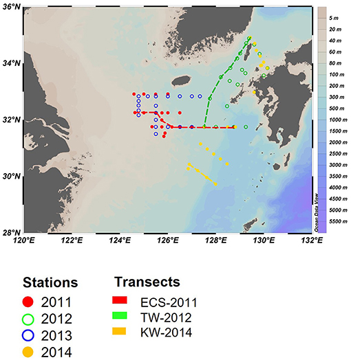
Figure 1. Sampling locations for the four cruises in the East China Sea (ECS) and Tsushima Strait (TS) in late July of 2011 and 2014. Three transects (dashed line) and three representative stations (inverted triangle) in Changjiang diluted water (St-CDW), Tsushima water (St-TW), and Kuroshio water (St-KW) were selected to compare vertical profiles of water properties and phytoplankton distributions.
Surface water samples for CHL, phytoplankton pigments, and nutrients (including DIN = NO3− + NO2−, DIP: ) were collected using an acid-washed bucket. Nutrient samples were immediately frozen in polyethylene tubes and transferred to the shore laboratory under frozen conditions for analysis using an Auto-Analyzer (AACS-IV, BLTEC). DIN and DIP concentrations were determined according to absorption spectrometry (Murphy and Riley, 1962; Armstrong et al., 1967; Koroleff, 1983). The observation area in 2013 was overlapped with 2011, therefore three transects (ECS-2011, TW-2012, and KW-2014) in the featured region were selected to show the differences in regional water mass properties and phytoplankton communities of the euphotic water column (Figure 1).
Sea surface temperature (SST) and MODIS/Aqua CHL were obtained from the NASA Ocean Color website (http://oceancolor.gsfc.nasa.gov/). Monthly composites for our study area (122–132°N, 28–36°E), for July 2011, 2012, and 2014, were extracted from global coverage datasets.
Estimation of Phytoplankton Communities From Pigment Concentration
Water samples for HPLC pigment analysis (1–2 L) were filtered onto 25 mm Whatman GF/F glass fiber filters under a vacuum pressure (<0.01 MPa) and dim light and immediately frozen in liquid nitrogen for measurement in the laboratory. Concentrations of 19 pigments were measured using KANSO CO. LTD. according to the method suggested by Van Heukelem and Thomas (Van Heukelem and Thomas, 2001) using reverse-phase HPLC with a Zorbax Eclipse XDB-C8 column (150 × 4.6 mm, 3.5 μm; Agilent Technologies, USA FluoroProbe (bbe moldaenke, Germany)).
CHEMTAX was used to interpret phytoplankton group composition based on pigment data. Matrices of pigment data and initial pigments/CHL ratio for each phytoplankton group were used as input of the CHEMTAX program (Mackey et al., 1996). Thirteen marker pigments were selected and classified into nine phytoplankton groups according to published papers in the ECS and adjacent areas (Furuya et al., 2003; Zhu et al., 2009; Liu et al., 2016). Samples were separated into different subsets according to their similarity of pigment compositions by clustering analysis to ensure that the pigment ratios were constant for CHEMTAX analysis. For each dataset, the CHEMTAX program was run 10 times using the output ratio matrix of the last run as the next ratio matrix input, and the optimized phytoplankton compositions were selected from the most stable final ratios among the 10 outputs (Latasa, 2007). More details on deriving the appropriate proportions of phytoplankton groups from CHL, using the CHEMTAX program, are described in detail in our earlier work (Gomes et al., 2018).
Estimation of Phytoplankton Communities From Fluorescence Excitation Spectra
After vertical profiles of phytoplankton excitation spectra were collected using the Multi-Exciter, the model suggested by Wang et al. (2016) was applied to estimate phytoplankton groups from the measured fluorescence spectra. In brief, this model includes three steps: (1) Continuum removal and band ratio were processed to obtain spectral features from phytoplankton fluorescence excitation spectra F(λ), which are associated with the composition of phytoplankton groups. (2) Principle component analysis (PCA) was used to compress the redundancy of spectral features and to obtain PC scores, which were used to derive the CHL fractions of the phytoplankton groups. (3) A sigmoid function was used to estimate phytoplankton groups from spectral data as:
where f denotes CHL fractions of brown algae, cyanobacteria, or green algae; Si is the i-th PC score; c0 and ci are regression coefficients between phytoplankton group fractions and PC scores (Si); k is the number of PCs, which was set to 8 because 99% of the variance of the original dataset can be explained by the first 8 PC scores.
In this study, four groups were determined according to the spectral characteristics of each group (brown algae, cyanobacteria, green algae, and cryptophytes). The upper and lower limits of f were set as 1 and 0, respectively, to avoid unrealistic estimates. Cryptophytes were calculated as 1–fbrown algae-fcyanobacteria-fgreen algae by considering that the sum of four phytoplankton groups is 1. More details of the model can be found in Wang et al. (2016). Datasets from 2011 to 2013 are obtained from the study by Wang et al. (2016), which, after calibration, showed statistically high relationships with CHEMTAX-derived phytoplankton groups (R2 = 0.64, 0.68, 0.36, and 0.49 and RMSE = 0.117, 0.078, 0.072, and 0.060 for brown algae, cyanobacteria, green algae, and cryptophytes, respectively). Data from 2014 were recalibrated with HPLC samples collected in the same year to improve the accuracy of the model. Correlation coefficients (R2) varied from 0.72, 0.87, 0.61, and 0.19 and RMSE were <0.2 for brown algae, cyanobacteria, green algae, and cryptophytes, respectively.
Results
Water Mass Properties
Surface SST and CHL
Satellite imagery was used to compare interannual variations in SST and CHL in the ECS and TS in July for 3 years. SST was higher than 30°C at low latitudes around 32°N and decreased to <25°C, north of 34°N during all 3 years (Figures 2a–c). High SST during each year was associated with the pathway of Kuroshio current flowing southeast of the ECS. In the region influenced by the Kuroshio, SST varied only slightly over 3 years, but relatively higher temperatures and wider ranges were observed south of Kyushu Island in 2012 (Figure 2b). Along the Chinese coast, high-temperature water (>30°C) was observed nearshore, in the Changjiang estuary, but in the north of the Changjiang estuary, low temperatures (<25°C) were recorded.
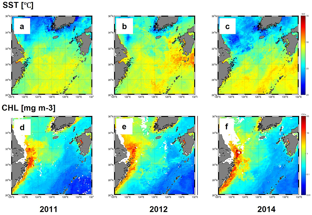
Figure 2. Monthly composites of SST (°C) (a–c) and CHL (mg m-3) (d–f) in the ESC 9 and TS during 2011-2014 in July.
The CHL concentrations were high (>5 mg m−3) along the coast and adjacent areas but decreased sharply offshore, where low values (<0.1 mg m−3) were recorded in the Kuroshio region (Figures 2d–f). In 2014, a broad swath of high CHL (>1 mg m−3) extended northward into the Yellow Sea in 2012, a feature not observed in the other two years (Figure 2e).
Delineation of Eater Masses Based on T-S Plots
Four major water masses were defined by a temperature vs. salinity (T-S) plot for samples from the upper 100 m in our study areas (Figure 3). Previous studies (Zhang et al., 2007; Zhou et al., 2008) have defined the CDW as low salinity (<30) and temperature ≥23°C. These included waters from the upper layer (depth < 15 m) and for stations sampled in 2011, 2013, and for one station in 2014. The KW was characterized by salinities >34 and distinctive high temperatures, although the shallow layers are potentially mixed with coastal water of lower salinity (Gong et al., 1996; Umezawa et al., 2014). For this study, the KW was defined by high salinity (>32.9) and high temperature (≥23°C), characteristics that were observed from 0 to 65 m, including the stations that were sampled in 2012 and 2014. A cold-water mass with a temperature <19°C was observed from 20 to 40 m in 2011 and 2013, and from 40 to 65 m in 2012 and 2014, and these waters were designated as Kuroshio subsurface water (KSSW). The water masses in between these three were marked as mixed waters.
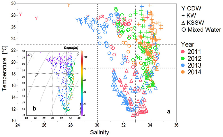
Figure 3. (a) Temperature-salinity (T-S) plot of the upper 100 m depth delineating water masses. CDW (Y) were defined as T > 23°C, S < 30, KW (+) were defined as T > 23°C, S >= 32.9, KSSW (Δ) were defined as T <19°C, and the rest data were defined as Mixed Water (O). (b) Depth of the samples of the T-S plot.
From the distribution of each water mass (Figure 4) and the depth of each water mass (Figure 3), the surface waters west of ECS in 2011 and 2013 were classified as CDW and KSSW at depth (Figures 4a,b); KW-covered areas east of the ECS and TS and KSSW were found in the central ECS, extending northward toward the western side of TS (Figures 4b,c).
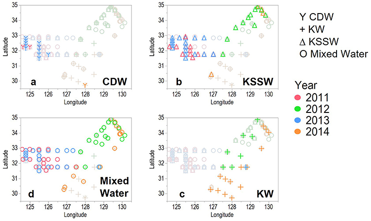
Figure 4. Distribution of each water mass (a: CDW, b: KSSW, c: KW, d: Mixed Water) that defined in Figure 3 in the study areas.
Vertical Observations
Temperature and Salinity
Strong stratification of the water column was observed in 2011, along a west to east transect (124.6°E to 128.8°E; ECS-2011) (Figure 5). A thermocline was detected at around 10–20 m in the west but at deeper layers toward the east indicating the presence of a northward-flowing Kuroshio branch at eastern stations. Cold bottom water was observed at the central stations, indicated by a sharp decrease in temperature to <15°C below the thermocline (Figure 5a). Salinity was >33 at depths deeper than 40 m, whereas large variations (28–33) were observed in the upper layers specifically in the western stations strongly influenced by low salinity CDW (salinity < 30). Waters strongly characteristic of the CDW with strong stratification were observed in the upper 10 m (Figure 5d).
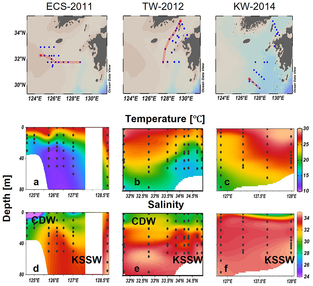
Figure 5. Vertical distributions of temperature (°C) (a–c), salinity (d–f) in the tree selected transects. Black dots represent sampling data.
Along transect TW-2012, low salinity water was observed in both the southern and northern stations in the upper 10 m indicating the influence of ECS water that was transported from ECS to TS along Kuroshio from 32°N to 34°N (Figure 5e). In the middle of the transect (32.5–33.5°N), salinities were higher with values of about 32.5 in the upper layers. The core of Kuroshio water (KW) was indicated by high salinity water (33.0–34.5) below 50 m in the south (~32.5°N), and but it rose to about 30 m in the north (~33.5°N) (Figure 5e). High temperature (>25°C) waters at southern stations extended to deeper waters up to 30 m but decreased sharply to 16°C at 70 m. A cold-water mass was observed at much shallower depths of around 30 m at the northern stations (~34°N) (Figure 5b). As a result, variations in the temperature at TS-2012 formed a deep thermocline at 50 m in the south, which gradually rose to the shallower depths, around 20 m when it moved northward (Figure 5b).
In transect KW-2014, high salinity (S > 33) and high temperature (T > 25) KWs characterized the most water column (Figure 5c). The eastern side around 128°E was especially characterized by surface temperatures higher than 29°C and bottom salinities higher than 34. However, low salinity water (salinity < 30) was observed in surface waters of the eastern stations (Figure 5f).
Nutrient Concentrations
Along ECS-2011, high DIN (>15 μM) and SiO2 (>6 μM), but low DIP (<0.1 μM), concentrations and high N:P ratios >50 were associated with the low salinity CDW, which extended up to 10 m at the 2 westernmost stations (Figures 6a,d,g,j). DIN and DIP were depleted in the upper layers at other offshore stations, whereas high SiO2 (>6 μM) was measured at all stations and depths except the KW region (128.5°N). High DIN and DIP were measured at deeper layers, forming a nitracline at about 20–80 m from the nearshore CDW stations and extending to the offshore KW stations (Figures 6a,g). The N:P ratios were generally less than those observed below the nitracline, except for high values observed at eastern stations where KSSW flowed (Figure 6j).
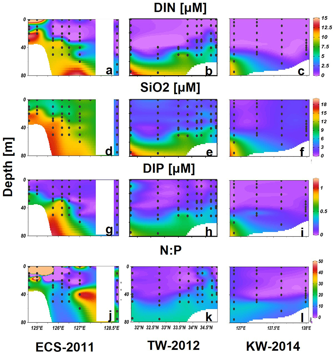
Figure 6. Vertical distributions of DIN (a–c), SiO2 (d–f), DIP (g–i) (μM), and N:P (j–l) in the tree selected transects. Black dots represent sampling data.
Both DIN and DIP were generally depleted in upper layers of transect TW-2012, with N:P ratios <10 (Figures 6b,h). A nitracline formed around 40–50 m from south to north. Noticeably, high DIN and DIP waters were found from 20 to 40 m with relatively higher N:P ratios (>16) in upper layers in northern stations. SiO2 was much lower (<3 μM) than that were observed in the ECS-2011 (Figures 6d,e).
Transect KW-2014 showed similar low nutrient concentrations in upper layers as TW-2012. High nutrients (DIN > 9, DIP > 0.6) were only measured in the deeper layer (>60 m) of the one station in the east. The N:P ratios were close to 16 in deep waters (depth > 50 m) of this transect (Figures 6c,f,i,l).
Phytoplankton Communities
Vertical profiles recorded to 80 m revealed the existence of a subsurface chlorophyll maxima (SCM) at all stations along ECS-2011 and TS-2012 (Figures 7a,b). In ECS-2011, the depth of SCM was only around 14 m (CHL = 6.75 mg m−3) at western stations but deeper observed around 65 m (CHL = 1.03 mg m−3) at the eastern station (Figure 7a). A double-SCM (CHL= 3.22 mg m−3 at 25 m; CHL = 3 mg m−3 at 50 m) was observed at station 127°E. Brown algae accounted for 60% of the CHL in SCM (Figure 7d), cyanobacteria were also dominant in the upper layers above the SCM (40–80%) (Figure 7g), and green algae and cryptophytes composed up to 20–40% of the CHL below the SCM (Figures 7j,m). Generally, surface and deep waters of coastal areas had distinct phytoplankton groups, whereas, at offshore stations, cyanobacteria and brown algae dominated, especially at stations along 126.5°N.
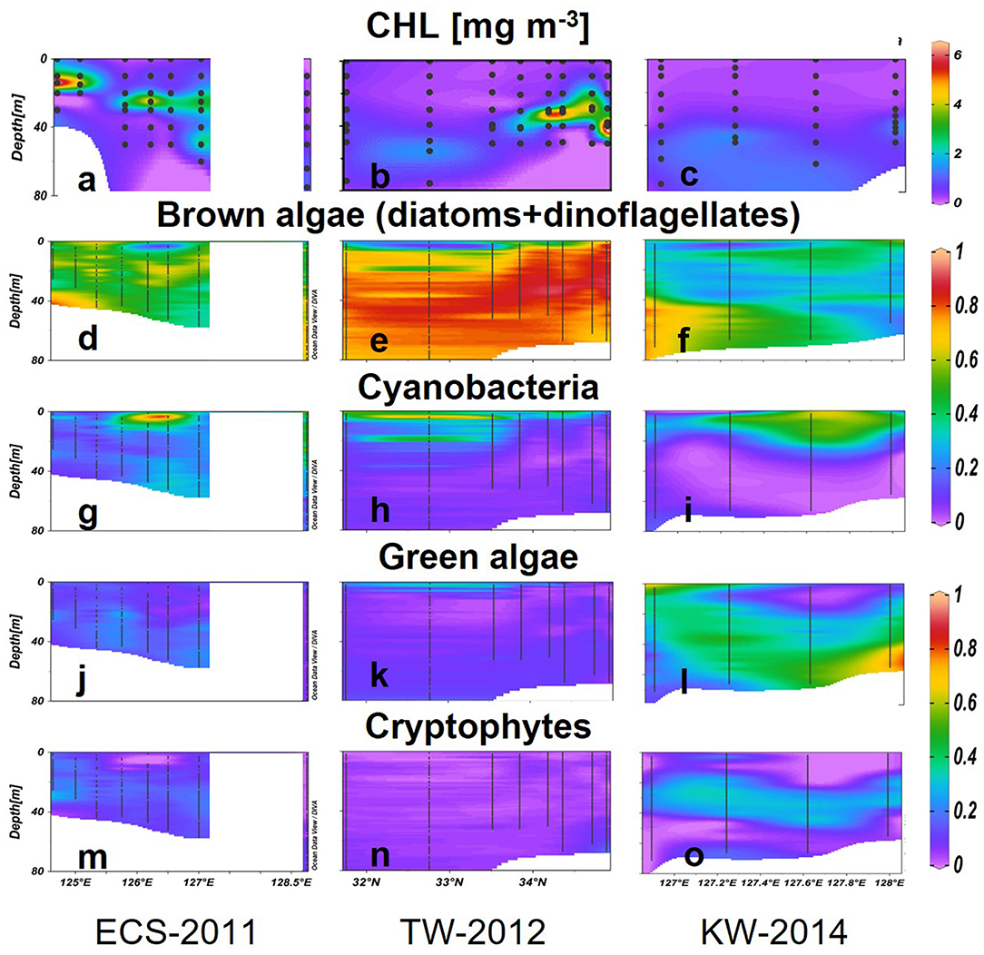
Figure 7. CHL (mg m−3) concentrations (a–c) and the relative abundance of phytoplankton groups (g–o) estimated using the Multi-Exciter in the three selected transects. Black dots represent sampling data.
In TW-2012, SCMs were deeper around 40–50 m from the south (32.75°N) to the north (Figure 7b). The CHL concentrations in the SCMs varied between 1.64 and 8.42 mg m−3, and the highest value was observed at the northern station around Tsushima Island (34.7°N). Relatively shallower SCMs were observed in the central stations at 34.1–34.7°N. Brown algae dominated the water column except just above the SCM, where cyanobacteria predominated (>30%) (Figures 7e,h). Above the SCM, the large (>40%) cyanobacterial populations were also found in the subsurface depth at around 20 m (Figure 7h). Green algae contributed 20% to the surface CHL but were lower at deeper depths. Cryptophytes showed low abundance for the area (Figures 7k,n).
In KW-2014, waters deeper than 50 m showed relatively higher CHL (0.50–1.66 mg m−3) than upper waters (<0.40 mg m−3) (Figure 7c). Brown algae were dominant (up to 85%) in deeper high nutrient waters to the west but were gradually replaced by green algae at eastern stations (Figures 7f,l). Cyanobacteria-dominated surface waters comprise more than 60% of the low CHL waters (Figures 7f,i). Cryptophytes were observed at around 20–50 m from west to east of this section (Figure 7o). A comparison between vertical profiles of phytoplankton groups derived from HPLC-CHEMTAX and Multi-Exciter derived is shown in Figure 9. The results from the two methods were generally consistent, i.e., brown algae and cyanobacteria showed high values in deep and surface layers, respectively; green algae showed a high value in the deep layer of the eastern station in 128°E (Figure 9, right). In addition, the high-resolution fluorescence profiles provided greater detail of the distribution patterns of phytoplankton groups than is possible by HPLC-CHEMTAX pigment analysis alone.
Discussion
Vertical Observations in the ECS and TS
This study focused on the vertical structure and variability of water masses and their influence on phytoplankton communities in the ECS and TS. Surface ocean color CHL images for the four summers that comprised our study revealed high CHL near Changjiang estuary, gradually decreasing offshore (Figure 2). These spatial distribution patterns are highly consistent with previous studies (Yamaguchi et al., 2012, 2013). However, our study reveals that besides surface variations, there are large changes in temperature and CHL with depth that needed to be examined, to understand how the movement of water masses in deeper layers can affect phytoplankton composition (Furuya et al., 2003; Liu et al., 2012).
The eastern ECS generally maintains its characteristics of oceanic waters, the KW flows into the ECS forming a mixture of water masses with CDW and water from the Yellow Sea, flowing further into the TS as TW (Isobe et al., 2002). In the ECS, high temperature, low salinity, and high N:P ratios were observed above 20 m indicating the influence of CDW. SCMs were located in the upper waters <30 m (Figures 8a–g). The phytoplankton groups varied annually: brown algae dominated in 2013, while mixed phytoplankton communities were recorded in 2011 (Figures 8h–k). CDW flowing into the mid-shelf of the ECS caused DIP-limitation and strongly inhibited the growth of large phytoplankton such as diatoms and dinoflagellate (denoted as brown algae in this study) (Wang et al., 2014, Wang et al., 2016; Gomes et al., 2018; Xu et al., 2019; Ishizaka, 2021). Similar patterns were reported for surface CDW dominated waters suggested by Xu et al. (2019) who suggested dominance by brown algae in 2013 was likely caused by the offshore movement of low N:P-ratio CDW to the mid-shelf ECS. At locations where vertical mixing was strong enough to erode the halocline, high salinity and high nutrient water that shoaled into the euphotic zone supported phytoplankton growth to form SCMs near the nitracline (Lee et al., 2017).
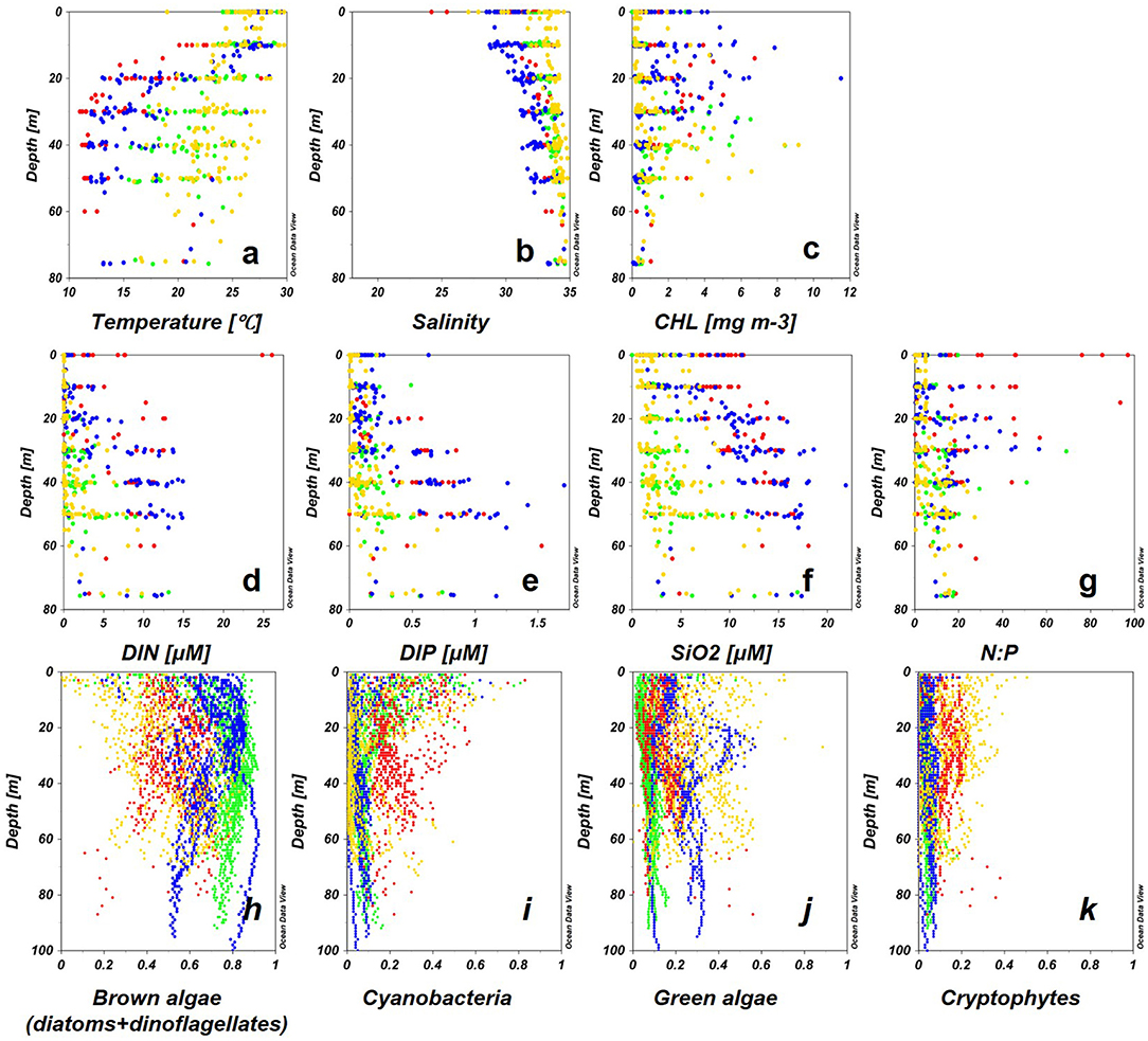
Figure 8. Vertical profiles of environmental factors (a–g) and Multi-Exciter-derived phytoplankton groups during the four courses (h–k), 2011: red, 2012: green, 2013: blue, 2014: yellow) for each water.
In TS (2012) and Kuroshio region (2014), surface CHL was low, and SCMs were recorded below 30 m (Figure 8c). Brown algae contributed to the high CHL in the entire euphotic column especially in SCM (Figure 8h). A previous study in TS showed that 70% of the freshwater at upper depths (<50 m) flowed from the ECS to TS, however, DIN and DIP had been depleted by the phytoplankton in the ECS (Isobe et al., 2002; Morimoto et al., 2009). Therefore, the dominance of brown algae represents a typical feature of phytoplankton composition in coastal regions of global oceans (Simpson and Sharples, 2012; Wang et al., 2014). In the Kuroshio region (2014), brown algae were replaced by green algae in the SCMs at deep depth. The paucity of nutrients in the surface waters of the Kuroshio region greatly limited the growth of large phytoplankton, but conversely facilitated the growth of small phytoplankton because of their high photosynthetic efficiency under stable light conditions (Ishizaka et al., 1994; Wang et al., 2014).
Application of Multiple Excitation Fluorometer on the Study of Phytoplankton Community Structure
Phytoplankton groups derived using multiple excitation fluorometer and calibrated with similar phytoplankton community distribution derived using in-situ HPLC pigment biomarkers offer two major advantages. First, this submersible profiling instrument was able to provide accurate high-resolution vertical profiles of phytoplankton in ECS and TS far greater than that possible by discrete depth HPLC-pigment samples (Figure 9, left). At almost all stations HPLC pigment analysis could not adequately capture the phytoplankton variability associated with different water masses. For example, temperature, nutrient, and CHL concentrations, all showed clear vertical and spatial changes (Figures 5c, 6c,f,i,l, 7c), but it was difficult the associated fine-scale changes in phytoplankton composition with HPLC derived phytoplankton groups (Figure 9, left). Conversely, the fluorometer provided phytoplankton abundance every 1 m (Figure 9, right) with general results that were consistent with HPLC-derived phytoplankton groups.
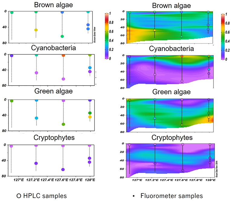
Figure 9. Comparison between HPLC-CHEMTAX (left) and the Multi-Exciter (right) derived vertical profiles of phytoplankton compositions. The colored dots were samples measured using the HPLC method; these samples overlayed on the profiles presented by the fluorometer and marked with black circles.
The interaction between water mass changes and phytoplankton variabilities was observed on a larger scale due to the large amount of data generated. Three transects were chosen to show the relative abundances of phytoplankton groups in KW (KW-2014), TS (TW-2012), and ECS (ECS-2011). Even in KW-2014, which was mostly affected by KW, temperature and nutrient gradients resulted in three layers of different phytoplankton groups. Surface and deep water were gradually mixed at 20–50 m, with temperatures of 22–24.5°C, and nutrient concentrations were low. Consequently, CHL in the surface waters was low, and cyanobacteria and green were the major contributors to CHL. Below 50 m, at the western and eastern stations, brown and green algae contributed to the higher CHL. Compared with KW-2014, section TW-2012 was mostly dominated by brown algae, but the shift to dominance by green algae (probably prochlorophytes, as discussed in the following paragraph) at the eastern station is probably related to the flow of low-nutrient, high-temperature KW (Liu et al., 2016; Ishizaka, 2021). This was well-captured by the fluorometer making possible large-scale observations, especially for retracing imperceptible variations, difficult to observe by sampling at discrete depths.
The objective of the Multi-Exciter calibration in our study is to extract spectral characteristics of different phytoplankton groups from in-situ HPLC CHEMTAX data. Compared with the initial calibration, the in-situ calibration in this study takes advantage to obtain spectral differences of each phytoplankton group without defining “norm spectra.” The “norm spectra” for the Multi-Exciter was initially calibrated by the manufacturing company with freshwater species cultured in the laboratory (Yoshida et al., 2011), similar to another multiple excitation fluorometer, the FluoroProbe. Several researchers who used the FluoroProbe pointed out that the accuracy of the fluorometer is largely dependent on the calibration (See et al., 2005; Richardson et al., 2010), and the determination of the norm spectra of each group is the fundamental component for evaluation (Beutler et al., 2002). It has been known that the norm spectra between species are not always the same under different environmental conditions and varied phytoplankton composition (Loftus and Seliger, 1975), which leads to under/overestimation by the fluorometer (Beutler et al., 2002; Alexander et al., 2012). Therefore, applying the present model facilitates using the Multi-Exciter without measuring cultured algae spectra from the specific study areas.
There are, however, some limitations to the use of multiple excitation fluorometers in the field. First, the fluorescent spectra data in shallow layers (<5 m in this study) were influenced by non-photochemical quenching under high light conditions, so that it cannot correctly reflect phytoplankton physiological properties and total abundance and species composition may be influenced (Koblížek et al., 2001; Morrison, 2003).
Second, our approach cannot resolve as many phytoplankton groups as HPLC-derived pigments in association with CHEMTAX. For example, in this study, prochlorophytes were not included for calibration, whereas this group was frequently observed in the Kuroshio region of the ECS (Furuya et al., 2003; Xu et al., 2019). Prochlorophytes, which are part of a cyanobacterial group, are about 0.6–0.8 μm in size and contain the dominant and characteristic pigment divinylchlorophyll a. The spectral shape of divinyl-chlorophyll a is similar to CHL, showing fluorescence emission in the red band, which overlaps with that of CHL (Zapata et al., 2000; Bricaud et al., 2004). The complementary pigments of prochlorophytes include chlorophyll b2, zeaxanthin, and α-carotene, which is a similar pigment composition to prasinoxanthin containing prasinophytes (Goericke and Repeta, 1992). The Multi-Exciter will detect this group as green algae rather than cyanobacteria. Our HPLC analysis of pigments shows that divinyl-chlorophyll a was present in the Kuroshio region (0.01–0.35 mg m−3), with maximum values in the SCM of KW-2014. The Multi-Exciter detected green algae in association with the high KW in mixed layers where temperature was around 22–24.5°C (Figures 5c, 7i). Therefore, the green algae detected using the Multi-Exciter in the KW region of 2014 should be revised as prochlorophytes, as previous studies have revealed that prochlorophytes was temperature-sensitive and restricted in KW in the eastern ECS (Lee et al., 2014; Ishizaka, 2021). This example serves to stress the necessity and importance of using a combination of Multi-Exciter and HPLC pigment analysis at certain depths to ascertain the whole structure of phytoplankton groups.
Conclusion
In this study, we used a newly developed multiple excitation fluorometer to estimate the vertical distribution of phytoplankton groups in the ECS and TS. Compared with the historical approach of pigment biomarkers derived using HPLC separation of phytoplankton pigments, the in-situ fluorometer provided a very large dataset of high resolution, vertical profiles of phytoplankton groups, which allowed us to infer their relationship with different water masses. Cyanobacteria were highly associated with low-CHL KW both spatially and vertically. Brown algae dominated the TW showing the features of the coastal waters. Green algae and cryptophytes were regionally distributed: cryptophytes contributed to the deeper layers of SCM in CDW and KW possibly influenced by nutrient and light conditions, and prochlorophytes were found in association with the high-temperature KW. Overall, the newly developed in-situ multiple excitation fluorometer successfully detected phytoplankton groups in both coastal and oceanic waters and provided high-resolution profile data making observations of large-scale variations in phytoplankton groups in association with dynamic water masses an exciting possibility.
Data Availability Statement
The original contributions presented in the study are included in the article/supplementary material, further inquiries can be directed to the corresponding author/s.
Author Contributions
QX: conceptualization, methodology visualization, and writing. JI: project administration, supervision, and funding acquisition. SY: project administration and conceptualization. YW: validation. YZ, YX, and JL investigation. TM: project administration and funding acquisition. JG and HG: conceptualization, writing—review, and editing. CS: validation and resources. SW: methodology, software, and validation. All authors contributed to the article and approved the submitted version.
Funding
This study was supported by JAXA GCOM-C project and Northwest Pacific Region Environmental Cooperation Center for the support of the Northwest Pacific Action Plan (NOWPAP) of the United Nations Environment Programme to JI, and JSPS KAKENHI grant number JP26241009 to TM. The participation of JG and HR was supported by NSF #2019983 and NASA Grants CMS-80NSSC20K0014 0014, GLIMR-143512. The participation of SW was supported by the National Natural Science Foundation of China (No. 42176181). The participation of YZ was partially supported by the Zhejiang Provincial Public Welfare Technology Application Research Program of China under Grant No. LGF21D060001 and the Scientific Research Fund of the Second Institute of Oceanography, MNR (JG2012). The participation of SY was supported by KIMST (MOF) #1525010982.
Conflict of Interest
YW was employed by the General Environmental Technos Co. Ltd.
The remaining authors declare that the research was conducted in the absence of any commercial or financial relationships that could be construed as a potential conflict of interest.
Publisher's Note
All claims expressed in this article are solely those of the authors and do not necessarily represent those of their affiliated organizations, or those of the publisher, the editors and the reviewers. Any product that may be evaluated in this article, or claim that may be made by its manufacturer, is not guaranteed or endorsed by the publisher.
Acknowledgments
We would like to thank the captains and crews of T/V Nagasaki-maru for their support during the cruises.
References
Alexander, R., Njuru, P., and Imberger, J. (2012). Identifying spatial structure in phytoplankton communities using multi-wavelength fluorescence spectral data and principal component analysis. Limnol. Oceangr. Methods 10, 402–415. doi: 10.4319/lom.2012.10.402
Armstrong, F. A. J., Stearns, C. R., and Strickland, J. D. H. (1967). The measurement of upwelling and subsequent biolog-ical processes by means of the Technicon Autoanalyzerand associated equipment. Deep Sea Res A. 14, 381–389.
Beutler, M., Wiltshire, K. H., Meyer, B., Moldaenke, C., Lüring, C., Meyerhöfer, M., et al. (2002). A fluorometric method for the differentiation of algal populations in vivo and in situ. Photosyn. Res. 72, 39–53. doi: 10.1023/A:1016026607048
Bricaud, A., Claustre, H., Ras, J., and Oubelkheir, K. (2004). Natural variability of phytoplanktonic absorption in oceanic waters: Influence of the size structure of algal populations. J. Geophys. Res. Oceans 109:C11. doi: 10.1029/2004JC002419
Chen, C. T. A. (2008). Distributions of nutrients in the East China Sea and the South China Sea connection. J. Oceanogr. 64, 737–751. doi: 10.1007/s10872-008-0062-9
Fujiwara, A., Nishino, S., Matsuno, K., Onodera, J., Kawaguchi, Y., Hirawake, T., et al. (2018). Changes in phytoplankton community structure during wind-induced fall bloom on the Chukchi Shelf. Polar Biol. 41, 1279–1295. doi: 10.1007/s00300-018-2284-7
Furuya, K., Hayashi, M., Yabushita, Y., and Ishikawa, A. (2003). Phytoplankton dynamics in the East China Sea in spring and summer as revealed by HPLC-derived pigment signatures. Deep Sea Res Part II Top Stud Oceanogr. 50, 367–387. doi: 10.1016/S0967-0645(02)00460-5
Ghadouani, A., and Smith, R. E. (2005). Phytoplankton distribution in lake erie as assessed by a new in situ spectrofluorometric technique. J. Great Lakes Res. 31, 154–167. doi: 10.1016/S0380-1330(05)70311-7
Goericke, R., and Repeta, D. J. (1992). The pigments of Prochlorococcus marinus: The presence of divinylchlorophyll a and b in a marine procaryote. Limnol. Oceanogr. 37, 425–433. doi: 10.4319/lo.1992.37.2.0425
Goes, J. I., do Rosario Gomes, H., Chekalyuk, A. M., Carpenter, E. J., Montoya, J. P., Coles, V. J., et al. (2014). Influence of the Amazon River discharge on the biogeography of phytoplankton communities in the western tropical north Atlantic. Prog. Oceanogr. 120, 29–40. doi: 10.1016/j.pocean.2013.07.010
Gomes, H. D. R., Xu, Q., Ishizaka, J., Carpenter, E. J., Yager, P. L., and Goes, J. I. (2018). The influence of riverine nutrients in niche partitioning of phytoplankton communities-a contrast between the Amazon River Plume and the ChangJiang (Yangtze) River diluted water of the East China Sea. Front. Mar. Sci. 5:343. doi: 10.3389/fmars.2018.00343
Gong, G. C., Chen, Y. L. L., and Liu, K. K. (1996). Chemical hydrography and chlorophyll a distribution in the East China Sea in summer: implications in nutrient dynamics. Cont. Shelf Res. 16, 1561–1590. doi: 10.1016/0278-4343(96)00005-2
Ishizaka, J. (2021). 3.2 Phytoplankton, in Oceanography of the Yellow Sea and East China Sea. Sidney, BC: North Pacific Marine Science Organization.
Ishizaka, J., Kiyosawa, H., Ishida, K., Ishikawa, K., and Takahashi, M. (1994). Meridional distribution and carbon biomass of autotrophic picoplankton in the Central North Pacific Ocean during Late Northern Summer 1990. Deep-Sea Res. Part I: Oceanogr. Res. Papers 41, 1745–1766. doi: 10.1016/0967-0637(94)90071-X
Isobe, A., Ando, M., Watanabe, T., Senjyu, T., Sugihara, S., and Manda, A. (2002). Freshwater and temperature transports through the Tsushima-Korea Straits. J. Geophys. Res. Oceans 107, 2–1. doi: 10.1029/2000JC000702
Jeffrey, S. W., and Vesk, M. (1997). “Introduction to marine phytoplankton and their pigment signatures,” in Phytoplankton Pigments in Oceanography, eds Jeffrey, S. W., Mantoura, R. F. C., and Wright, S. W., SW (Paris: UNESCO Publishing).
Koblížek, M., Kaftan, D., and Nedbal, L. (2001). On the relationship between the non-photochemical quenching of the chlorophyll fluorescence and the Photosystem II light harvesting efficiency. A repetitive flash fluorescence induction study. Photosynth. Res. 68, 141–152. doi: 10.1023/A:1011830015167
Koroleff, F. (1983). “Determination of silicon,” in Methods of Seawater Analysis, eds Glasshoff, K., Ehrhardt, M., and Kremling, K., (Weinheim: Verlag Chemie).
Latasa, M. (2007). Improving estimations of phytoplankton class abundances using CHEMTAX. Mar Ecol Prog Ser. 329, 13–21. doi: 10.3354/meps329013
Lee, K., Matsuno, T., Endoh, T., Ishizaka, J., Zhu, Y., Takeda, S., et al. (2017). A role of vertical mixing on nutrient supply into the subsurface chlorophyll maximum in the shelf region of the East China Sea. Cont. Shelf Res. 143, 139–150. doi: 10.1016/j.csr.2016.11.001
Lee, Y., Choi, J. K., Youn, S., and Roh, S. (2014). Influence of the physical forcing of different water masses on the spatial and temporal distributions of picophytoplankton in the northern East China Sea. Cont. Shelf Res. 88, 216–227. doi: 10.1016/j.csr.2014.08.001
Liu, X., Huang, B., Liu, Z., Wang, L., Wei, H., Li, C., et al. (2012). High-resolution phytoplankton diel variations in the summer stratified central Yellow Sea. J. Oceanogr. 68, 913–927. doi: 10.1007/s10872-012-0144-6
Liu, X., Xiao, W., Landry, M. R., Chiang, K. P., Wang, L., and Huang, B. (2016). Responses of phytoplankton communities to environmental variability in the East China Sea. Ecosystems 19, 832–849. doi: 10.1007/s10021-016-9970-5
Loftus, M. E., and Seliger, H. H. (1975). Some limitations of the in vivo fluorescence technique. Chesapeake Sci. 1975, 79–92. doi: 10.2307/1350685
Mackey, M. D., Mackey, D. J., Higgins, H. W., and Wright, S. W. (1996). CHEMTAX-a program for estimating class abundances from chemical markers: application to HPLC measurements of phytoplankton. Mar. Ecol. Prog. Ser. 144, 265–283. doi: 10.3354/meps144265
Morimoto, A., Takikawa, T., Onitsuka, G., Watanabe, A., Moku, M., and Yanagi, T. (2009). Seasonal variation of horizontal material transport through the eastern channel of the Tsushima Straits. J. Oceanography 65, 61–71. doi: 10.1007/s10872-009-0006-z
Morrison, J. R. (2003). In situ determination of the quantum yield of phytoplankton chlorophyll a fluorescence: A simple algorithm, observations, and a model. Limnol. Oceanogr. 48, 618–631. doi: 10.4319/lo.2003.48.2.0618
Murphy, J. A. M. E. S., and Riley, J. P. (1962). A modified single solution method for the determination of phosphate in natural waters. Anal. Chim. Acta 27, 31–36. doi: 10.1016/S0003-2670(00)88444-5
Pires, M. D. (2010). Evaluation of Fluorometers for the in situ Monitoring of Chlorophyll and/or Cyanobacteria; Project Report, Deltares, Delft, Netherlands. Available online at: https://publications.deltares.nl/1203593_000.pdf
Richardson, T., Lawrenz, E., Pinckney, J., Guajardo, R. C., Waler, E. A., Paerl, H. W., et al. (2010). Spectral fluorometric characterization of phytoplankton community composition using the Algae Online Analyser. Water Res. 44, 2461–2472. doi: 10.1016/j.watres.2010.01.012
Rolland, A., Rimet, F., and Jacquet, S. (2010). A 2-year survey of phytoplankton in the Marne Reservoir (France): a case study to validate the use of an in situ spectrofluorometer by comparison with algal taxonomy and chlorophyll a measurements. Knowl. Manag. Aquat. Ecosyst. 398, 1–19. doi: 10.1051/kmae/2010023
See, J., Campbell, L., Richardson, T., Pinckney, J. L., Shen, R., Guinasso, J.r., et al. (2005). Combining new technologies for determination of phytoplankton community structure in the northern Gul of Mexico. J. Phycol. 41, 305–310. doi: 10.1111/j.1529-8817.2005.04132.x
Simpson, J. H., and Sharples, J. (2012). Introduction to the Physical and Biological Oceanography of Shelf Seas. Cambridge: Cambridge University Press. doi: 10.1017/CBO9781139034098
Uitz, J., Stramski, D., Reynolds, R. A., and Dubranna, J. (2015). Assessing phytoplankton community composition from hyperspectral measurements of phytoplankton absorption coefficient and remote-sensing reflectance in open-ocean environments. Remote Sens. Environ. 171, 58–74. doi: 10.1016/j.rse.2015.09.027
Umezawa, Y., Yamaguchi, A., Ishizaka, J., Hasegawa, T., Yoshimizu, C., Tayasu, I., et al. (2014). Seasonal shifts in the contributions of the Changjiang River and the Kuroshio Current to nitrate dynamics in the continental shelf of the northern East China Sea based on a nitrate dual isotopic composition approach. Biogeosciences 11, 1297–1317. doi: 10.5194/bg-11-1297-2014
Van Heukelem, L., and Thomas, C. S. (2001). Computer-assisted high-performance liquid chromatography method development with applications to the isolation and analysis of phytoplankton pigments. J Chromatogr A. 910, 31–49. doi: 10.1016/S0378-4347(00)00603-4
Wang, B., and Wang, X. (2007). Chemical hydrography of coastal upwelling in the East China Sea. Chin. J. Oceanol. Limnol. 25, 16–26. doi: 10.1007/s00343-007-0016-x
Wang, S., Xiao, C., Ishizaka, J., Qiu, Z., Sun, D., Xu, Q., et al. (2016). Statistical approach for the retrieval of phytoplankton community structures from in situ fluorescence measurements. Opt. Express 24, 23635–23653. doi: 10.1364/OE.24.023635
Wang, S. Q., Ishizaka, J., Yamaguchi, H., Tripathy, S. C., Hayashi, M., Xu, Y. J., et al. (2014). Influence of the Changjiang River on the light absorption properties of phytoplankton from the East China Sea. Biogeosciences. 11, 1759–1773. doi: 10.5194/bg-11-1759-2014
Wright, S., and Jeffrey, S. W. (2006). “Pigment markers for phytoplankton production,” in Marine Organic Matter: Biomarkers, Isotopes and DNA, ed Volkman, J., (Berlin: Springer). doi: 10.1007/698_2_003
Wright, S. W. (2005). “Analysis of phytoplankton populations using pigment markers,” in Course Notes for a Workshop “Pigment Analysis of Antarctic Microorganisms.” University of Malaya.
Xu, Q., Sukigara, C., Goes, J. I., do Rosario Gomes, H., Zhu, Y., Wang, S., et al. (2019). Interannual changes in summer phytoplankton community composition in relation to water mass variability in the East China Sea. J. Oceanogr. 75, 61–79. doi: 10.1007/s10872-018-0484-y
Yamaguchi, H., Ishizaka, J., and Siswanto, E. (2013). Seasonal and spring interannual variations in satellite-observed chlorophyll-a in the Yellow and East China Seas: new datasets with reduced interference from high concentration of resuspended sediment. Cont. Shelf Res. 59, 1–9. doi: 10.1016/j.csr.2013.03.009
Yamaguchi, H., Kim, H. C., Son, Y. B., Kim, S. W., Okamura, K., Kiyomoto, Y., et al. (2012). Seasonal and summer interannual variations of SeaWiFS chlorophyll a in the Yellow Sea and East China Sea. Prog. Oceanogr. 105, 22–29. doi: 10.1016/j.pocean.2012.04.004
Yamamoto, R., Harada, M., Hiramatsu, K., and Tabata, T. (2021). Three-layered Feedforward artificial neural network with dropout for short-term prediction of class-differentiated Chl-a based on weekly water-quality observations in a eutrophic agricultural reservoir. Paddy Water Environ. 2021, 1–18. doi: 10.1007/s10333-021-00874-3
Yoshida, M., Horiuchi, T., and Nagasawa, Y. (2011). In situ multi-excitation chlorophyll fluorometer for phytoplankton measurements: Technologies and applications beyond conventional fluorometers. Oceans 2011, 1–4. doi: 10.23919/OCEANS.2011.6107049
Zapata, M., Rodríguez, F., and Garrido, J. L. (2000). Separation of chlorophylls and carotenoids from marine phytoplankton: a new HPLC method using a reversed phase C8 column and pyridine-containing mobile phases. Mar. Ecol. Prog. Ser. 195, 29–45 doi: 10.3354/meps195029
Zhang, J., Liu, S. M., Ren, J. L., Wu, Y., and Zhang, G. L. (2007). Nutrient gradients from the eutrophic Changjiang (Yangtze River) Estuary to the oligotrophic Kuroshio waters and re-evaluation of budgets for the East China Sea Shelf. Prog. Oceanogr. 74, 449–478. doi: 10.1016/j.pocean.2007.04.019
Zhou, M. J., Shen, Z. L., and Yu, R. C. (2008). Responses of a coastal phytoplankton community to increased nutrient input from the Changjiang (Yangtze) River. Cont. Shelf Res. 28, 1483–1489. doi: 10.1016/j.csr.2007.02.009
Keywords: phytoplankton community, in-situ fluorometer, East China Sea, Changjiang River diluted water, Kuroshio, Tsushima Strait
Citation: Xu Q, Wang S, Sukigara C, Goes JI, Gomes HdR, Matsuno T, Zhu Y, Xu Y, Luang-on J, Watanabe Y, Yoo S and Ishizaka J (2022) High-Resolution Vertical Observations of Phytoplankton Groups Derived From an in-situ Fluorometer in the East China Sea and Tsushima Strait. Front. Mar. Sci. 8:756180. doi: 10.3389/fmars.2021.756180
Received: 10 August 2021; Accepted: 22 November 2021;
Published: 04 January 2022.
Edited by:
Ryan Rykaczewski, Pacific Islands Fisheries Science Center (NOAA), United StatesReviewed by:
Xin Liu, Xiamen University, ChinaMeilin Wu, South China Sea Institute of Oceanology, Chinese Academy of Sciences (CAS), China
Copyright © 2022 Xu, Wang, Sukigara, Goes, Gomes, Matsuno, Zhu, Xu, Luang-on, Watanabe, Yoo and Ishizaka. This is an open-access article distributed under the terms of the Creative Commons Attribution License (CC BY). The use, distribution or reproduction in other forums is permitted, provided the original author(s) and the copyright owner(s) are credited and that the original publication in this journal is cited, in accordance with accepted academic practice. No use, distribution or reproduction is permitted which does not comply with these terms.
*Correspondence: Qian Xu, a2l0dHl4cTkwMjVAaG90bWFpbC5jb20=