Modeling Oyster Reef Restoration: Larval Supply and Reef Geometry Jointly Determine Population Resilience and Performance

1. Introduction

Native oyster species are dominant ecosystem engineers, which provide a diverse suite of ecosystem services, including water filtration, food and habitat for various species, shoreline stabilization, coastal defense, and enhanced fisheries production (Cerco and Noel, 2007; Coen et al., 2007; Grabowski and Peterson, 2007; Grabowski et al., 2012). These species were once abundant worldwide, such as the eastern oyster Crassostrea virginica of the western Atlantic and Gulf of Mexico coasts (Winslow, 1881; Baylor, 1895). Unfortunately, native oysters have been nearly extirpated by overfishing, habitat degradation, disease and eutrophication (Rothschild et al., 1994; Jackson et al., 2001; Kirby, 2004; Lotze et al., 2006; Airoldi and Beck, 2007; Beck et al., 2011; Zu Ermgassen et al., 2012). Worldwide, 85% of native oyster reefs have been eradicated (Beck et al., 2011). Along the Pacific, Atlantic, and Gulf of Mexico coasts of North America, 88% of oyster biomass and 64% of reef area have been lost since the 1800s by the eastern oyster C. virginica and the Olympia oyster Ostrea lurida (Zu Ermgassen et al., 2012).

In Chesapeake Bay, abundance of the eastern oyster has been reduced to approximately 1% of its historical levels due to overfishing, oyster reef degradation, and disease (Rothschild et al., 1994; Wilberg et al., 2011; Schulte, 2017). Restoration efforts had failed through the start of the 21st century (Kennedy et al., 2011), but have proven successful since the mid-2000s due to the adoption of new restoration approaches in Chesapeake Bay (Schulte et al., 2009; Lipcius et al., 2015, 2019; Colden et al., 2016; Theuerkauf and Lipcius, 2016; Lipcius and Burke, 2018) and in other Atlantic coast estuaries (Taylor and Bushek, 2008; Powers et al., 2009), and in the Gulf of Mexico (La Peyre et al., 2014). These efforts are distinguishable from past failed attempts by their attention to key elements of habitat quality, such as the architecture and height of restoration reefs (Taylor and Bushek, 2008; Powers et al., 2009; Schulte et al., 2009; La Peyre et al., 2014; Lipcius et al., 2015), and to insights gained from population models.

Several modeling approaches have been utilized to inform oyster population dynamics, restoration and fishery management strategies, each with specific goals and approaches. Mechanistic, physiologically-based models were among the first to be employed to address issues regarding effects of environmental conditions and biotic processes such as food availability (Hofmann et al., 1992, 1994; Powell et al., 1992; Dekshenieks et al., 1993) and later to the effects of disease and environmental factors (Powell et al., 1995, 2011; Dekshenieks et al., 1996; Klinck et al., 2002; Hofmann et al., 2004; Lavaud et al., 2017). Similar models were subsequently used to address management strategies and dynamics of shell budgets on harvested oyster reefs (Powell et al., 2006, 2012, 2018; Powell and Klinck, 2007; Wilberg et al., 2013; Soniat et al., 2014). More recently, population models have been addressing issues related to oyster restoration, specifically the factors that promote long-term persistence and resilience of restoration reefs (Jordan-Cooley et al., 2011; Puckett and Eggleston, 2012; Pine et al., 2015; Housego and Rosman, 2016; Moore et al., 2016, 2018; DePiper et al., 2017; Lipcius et al., 2019; Yurek et al., 2021).

Some population models have integrated reef habitat quality (Jordan-Cooley et al., 2011; Wilberg et al., 2013; Housego and Rosman, 2016; DePiper et al., 2017; Lipcius et al., 2019; Yurek et al., 2021), and demonstrated that initial reef height is a key determinant of oyster population persistence and can lead to alternative states (i.e., reef degradation or persistence) for the eastern oyster in restoration (Jordan-Cooley et al., 2011; Housego and Rosman, 2016) and harvest (Wilberg et al., 2013; DePiper et al., 2017) reefs. Population dynamics of oysters and other invertebrates, such as corals, can differ as a function of age or stage (Moore et al., 2016, 2018) and the magnitude of recruitment (Colden et al., 2017; Edmunds and Riegl, 2020). Hence, a need exists to incorporate stage or age structure and recruitment variation in models of eastern oyster population dynamics to determine optimal reef geometries in restoration. Consequently, we modified our previous model (Jordan-Cooley et al., 2011) by separating the population into juvenile and adult stages, which allowed us to assess the influence of variable recruitment and sediment concentration on critical reef height for population persistence of eastern oyster on restoration reefs. We hypothesized that the critical reef height for population persistence is not constant in relation to sediment being deposited on a reef, and is related to the magnitude of larval supply and recruitment impinging on an oyster reef.

To evaluate the hypotheses, we first describe how we integrated the juvenile and adult elements of the stage-structured model. Next, we define the parameters and functions, and show how they were derived. Finally, we conduct numerical and bifurcation analyses of the model for initial reef height under differing levels of larval supply and sediment concentration to produce a comprehensive evaluation of population dynamics relevant for oyster restoration.

2. Stage-Structured Demographic Model

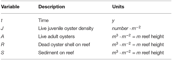
Our original model consisted of three differential equations that describe the interactions between live oyster volume, dead oyster shell volume in the reef, and sediment accumulation (Jordan-Cooley et al., 2011). We now revise the model to incorporate stage structure by splitting the live oyster equation into two equations, one for adult volume and another for juvenile density. The revised JARS (Juveniles, Adults, Reef, Sediment) model defines the change in juvenile oyster density J, adult oyster volume A, dead oyster shell volume R, and sediment volume S on a 1-m² reef patch as a function of time t in years. The units for A, R and S may be interpreted as a volume (m³) or as total reef height (m = m³ · m⁻²) because we are dealing with a 1-m² reef patch. See Figure 1 for a schematic of the system and Table 1 for a summary of variables.

FIGURE 1

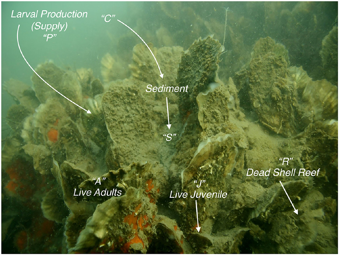
Figure 1. Representation of the main elements of the stage-structured JARS model; letters above each element match those in the model. Larval production P, larval supply, which includes larvae both from the natal population and from outside populations. C, water-column sediment concentration before being deposited on the reef. Photo by Stopher Slade; https://ncseagrant.ncsu.edu/coastwatch/previous-issues/2017-2/holiday-2017/making-the-most-of-oyster-reef-filtering/.

TABLE 1

Table 1. JARS model variables, description, and units.

2.1. Juvenile Oyster Density

The rate of change in live juvenile oyster density J in number per m² is:

$\begin{array}{ll}\frac{dJ}{dt}=P·L(A,R)·f(d_J)-J& (1)\end{array}$

where the first term represents the product of larval production (= supply) P, a larval recruitment function L(A, R), and a switching function f(d_J). The second term (−mJ) defines a loss through maturation of juveniles into adults. Larval production P represents availability of larvae to settle onto a reef (Connolly and Roughgarden, 1999). In our model, larval production is not explicitly linked to adult abundance on the natal reef, such that larval production implicitly includes larvae supplied from outside reefs and the natal reef.

The larval recruitment function L (i.e., the fraction of oyster larvae that can settle successfully, become juveniles, and survive to mature to the adult stage) is dependent upon the volume of live adult oysters A and the volume of dead oyster shell R, as:

$\begin{array}{ll}L(A,R)=\frac{\frac{A}{\psi }+{(\frac{R}{\psi })}^2}{\zeta +{(\frac{A}{\psi })}^{\theta }+{(\frac{R}{\psi })}^2},& (2)\end{array}$

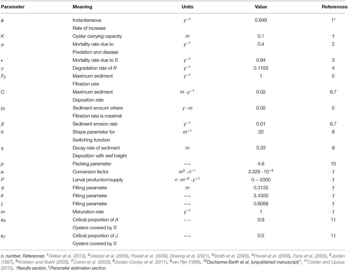
where ψ, ζ, and θ are fitting parameters (see Table 2 for list of parameters). In Figure 2, we display the form of the function L(A, R) with parameter values that best match field data. For a fixed R, larval recruitment with respect to A is a Ricker-type function (Schulte et al., 2009), such that recruitment peaks at some intermediate value of A and then decays as A → ∞ (Figure 2). Larval recruitment with respect to R, for fixed A, is a sigmoid function (Colden et al., 2017), which increases slowly at low dead oyster shell volume, then rises sharply before saturating asymptotically as R → ∞ (Figure 2). The sigmoid curve of recruitment increasing toward an asymptote with only dead shell was based on the data in Colden et al. (2017) when only shell was present on restoration reefs in the first year of the experiment. The effects of adults were based on Schulte et al. (2009) and on the second-year results in Colden et al. (2017) when adults were present. Moreover, because the dependence of recruitment on adult oysters is a Ricker-type function, which is linear at smaller values of adults, and the dependence on dead shell is sigmoidal, then small to moderate numbers of adults are more favorable to recruitment than dead shell. This collective effect upon recruitment thus accounts for the preference of pediveligers to settle amongst conspecifics.

TABLE 2

Table 2. Parameter values in the equations.

FIGURE 2

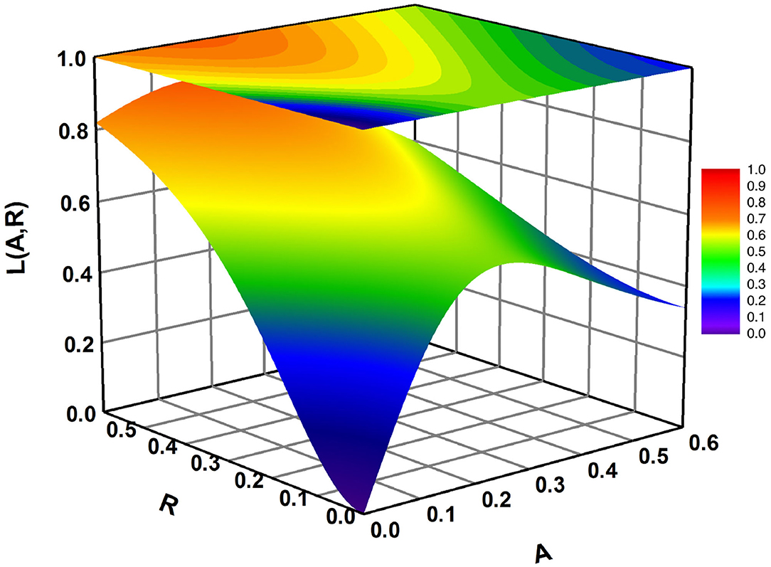
Figure 2. Larval recruitment L(A, R) (Equation 2) as a function of both A and R. Parameter values are in Table 2.

When $\zeta >\frac{\theta -1}{\theta }$, as is the case for our best fit parameters, L < 1 for any A, R ≥ 0 and L(A, R) can be interpreted as the fraction of available larvae that are successfully recruited and survive to adulthood. The parameter θ > 1 controls the behavior of decay with A; larger θ produces faster decay. The parameter ζ > 0 determines the height of the peak, while ψ > 0 defines the location of the peak. The collective effect of both functions is shown in Figure 2. The maturation term (−mJ) in Equation (1) contains a maturation rate m. Because the input term for the juvenile stage is larvae that are successfully recruited and will survive to adulthood, all of the J stage transitions to the adult stage.

2.2. Switching Functions

The proportion of oysters unaffected by sediment, which determines an effective population growth rate of juvenile or adult oysters, is given by a switching function:

$\begin{array}{ll}f(d_i)=\frac{1}{1+{\text{e}}^{-h{d}_i}},& (3)\end{array}$

where d_i = a_iA + R−S and i = J, A. Here d_J and d_A represent the volume of live oysters and dead oyster shell not affected by sediment on the reef, and a_A > a_J. The proportion of oysters not affected by sediment is an increasing function of d_A or d_J with a sigmoid shape bounded by 0 and 1 (Figure 3). When deposited sediment covers both the dead oyster shell (R) and a fraction a_i of the adult oyster volume (a_iA), d_i is near 0. When d_i > 0, live oysters are not significantly covered by sediment. The value of f(d_i) approaches 1 and the oysters can grow. In contrast, if more than a fraction a_i of the adult oysters are covered by sediment, then d_i < 0, f(d_i) approaches 0 and the oysters cannot grow. The same switching function was also used in Jordan-Cooley et al. (2011), but here the switching function for juveniles and adults differs in the parameters a_J and a_A, which set the burial threshold for detrimental effects of sediment on juveniles and adults, respectively. Specifically, the threshold for juveniles is much lower than that for adults (Table 2).

FIGURE 3

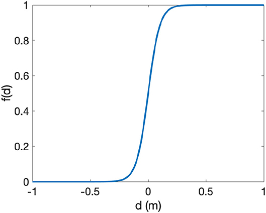
Figure 3. Switching function f(d) (Equation 3). Parameter values are in Table 2.

2.3. Live Adult Oyster Volume

The change in live adult oyster volume A is described by:

$\begin{array}{ll}\frac{dA}{dt}=\alpha mJ+\varphi A·f(d_A)\left(1-\frac{A}{K}\right)-\mu A·f(d_A)-ϵA·(1-f(d_A)).& (4)\end{array}$

The first term (αmJ) converts the number of matured juveniles to volume of adult oysters. The second term is the population growth rate of adult oysters, which like in the previous model (Jordan-Cooley et al., 2011) assumes live oysters follow logistic growth with an intrinsic growth rate ϕ and carrying capacity K. We call the growth rate parameter ϕ instead of r here because it represents only the positive change in biomass, and does not include the per capita mortality rate μ due to predation and disease incorporated in r (r = ϕ − μ). Population growth and mortality are scaled by a factor f(d_A), which is defined in Equation (3), since only oysters above the sediment can survive and reproduce. The last term represents the decrease in live adult oyster volume due to suffocation by sediments, where ϵ is the mortality rate of oysters covered by sediment. This term has a stronger effect as f(d_A) becomes smaller; i.e., when more oysters are covered in sediment.

2.4. Dead Oyster Shell Volume

The change of dead oyster shell volume R is modeled as:

$\begin{array}{ll}\frac{dR}{dt}=\mu A·f(d_A)+ϵA·(1-f(d_A))-\gamma R,& (5)\end{array}$

where the first two terms in the equation are directly from mortality of live oysters. The third term is the loss of dead oyster shell volume due to degradation, which is proportional to the volume of dead oysters at the rate γ. For simplicity, we do not include juveniles in the dead shell volume because they are small enough that they do not contribute significantly to shell volume (Lipcius et al., 2015).

2.5. Sediment Accumulation

The change in sediment volume S is:

$\begin{array}{ll}\frac{dS}{dt}=-\beta S+Cg·{\text{e}}^{-\frac{F(Cg)A}{Cg}},& (6)\end{array}$

where the first term represents the rate of sediment erosion, which is proportional to the volume of sediment on the reef at a rate β. The second term is the rate of sediment deposition. Without filtration by live oysters, the sediment deposition rate is Cg, where C is a maximum possible deposition rate and g is a modification function that decreases as reef height (A + R) increases. The rate of sediment deposition is maximized when there is no reef and no oysters, in which case the deposition rate is just C. Typical values of sediment deposition range from 0.00 to 0.02 m y⁻¹ (Cronin et al., 2003), which is why we chose a maximum rate for C of 0.02 m y⁻¹ (Table 2).

The parameter C is the sediment deposition rate from the water column (Figure 1), whereas the amount of sediment actually deposited and remaining on the reef is the variable S, which is a non-linear function of C. The effect of sediment on larval settlement and recruitment is implemented via the switching function f(d_i) in the input term of the juvenile equation. When the sediment height is small relative to the reef height, it is assumed that sediment has minimal effect on the larvae. However, f(d_i) causes the fraction of available larvae successfully recruited to decline as sediment increases, reflecting the realistic situation in nature.

A filtration rate function F scales down the deposition rate due to filtration of sediment by adult oysters A. The filtration function F and modification function g are defined by

$\begin{array}{ll}F(Cg)=\frac{F_{0}Cg}{y_0}{\text{e}}^{\frac{y_0-Cg}{y_0}},g(A+R)={\text{e}}^{-\eta (A+R)}.& (7)\end{array}$

The higher the filtration rate, the smaller the deposition rate. The filtration rate F scales linearly with Cg when Cg is small, reaches a peak filtration rate F₀ at some optimal sediment concentration y₀, and beyond this threshold, it decreases as oyster gills become increasingly clogged (Jordan-Cooley et al., 2011). The premise is to have a function bounded between 0 and 1 that peaks at some intermediate value and drops off exponentially. Graphs of g and F(Cg) are displayed in Jordan-Cooley et al. (2011).

In the Appendix, we show that a solution of Equations (1), (4), (5), and (6) with non-negative initial values is always non-negative and bounded; hence the model is mathematically well-posed.

3. Parameter Estimates

In the revised JARS model (Equations 1, 4, 5 and 6), some parameters come directly from field observations or the literature (Table 2), whereas others are approximated by fitting the functions with data from field restoration reefs, as described below. Although the model parameters were estimated from a limited number of sites in Chesapeake Bay, the selected sites are the best-studied, long-term restoration sites in the bay (Schulte et al., 2009; Lipcius et al., 2015, 2019; Colden et al., 2016; Theuerkauf and Lipcius, 2016).

3.1. Maturation Rate

We assume the average maturation time to adulthood is 1 year, such that the parameter m = 1 yr⁻¹. The maturation rate does not affect the equilibrium values of adults, reef or sediment because the input term in the juvenile equation is the rate at which juveniles are successfully recruited. All juveniles will eventually move into the adult stage regardless of the speed at which they do so, because the juvenile equation does not include mortality. Changing the maturation rate would only change the number of juveniles in our equilibrium results. However, it is conceivable that changing the maturation rate could affect transient dynamics. Using an extreme maturation rate of m = 3 yr⁻¹, we reran our calculation of the needed height of dead shell for successful restoration, and the results were virtually identical to those presented here.

3.2. Conversion of Juvenile Density to Oyster Volume

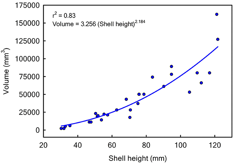
Since the units for juvenile oysters J and adult oysters A are numbers · m⁻² and m³ · m⁻² respectively, we needed a conversion factor α in Equation (4) to convert juvenile density into adult volume. To do so, we used shell height and volume data for 28 oysters from the field study of Lipcius et al. (2015). The data were log₁₀-transformed and analyzed with linear least-squares regression (Figure 4), yielding the following equation:

$\begin{array}{ll}V=3.256·S{H}^{2.184}& (8)\end{array}$

where V is shell volume in mm³ and SH is Shell Height in mm. From this relationship, we calculated the volume of one juvenile oyster using its shell height. We assumed that mean juvenile SH = 35 mm (Schulte et al., 2009). Using Equation (8), the volume of an average juvenile oyster is 3.256 · 35^2.184 · 10⁻⁹ = 7.6724 · 10⁻⁶ m³. When converting, we also needed to multiply the calculated juvenile volume by a packing parameter p (Ducharme-Barth et al., unpublished manuscript)¹, because the oysters are not all packed together and there is interstitial space between individuals. Using the packing parameter 4.6 (Ducharme-Barth et al., unpublished manuscript)¹, we scaled the volume with α = 7.6724 · 10⁻⁶ · 4.6 = 3.529 · 10⁻⁵ m³ per juvenile.

FIGURE 4

Figure 4. Oyster length to volume conversion function: volume in mm³ vs. shell height in mm.

3.3. Larval Recruitment Function

To estimate fixed parameter values for ψ, θ, and ζ in the larval recruitment function L(A, R) and site-dependent values for larval availability P (Equation 2), we used a Matlab function to fit data collected at different restoration sites in the Great Wicomico River (GWR) by Schulte et al. (2009), and in the Great Wicomico River, Linkhorn Bay (LB) and Broad Bay (BB) of the Lynnhaven River system by Colden et al. (2017). Our approach was to fit the predicted number of recruits PL(A, R) in each location and year to the observed number. Because successful recruitment occurred, we assumed sediment did not inhibit recruitment and thus ignored the switching function f(d) in the recruitment term of Equation (1).

Available data for adults were number · m⁻², which we converted to m³ · m⁻² as described above and assuming a mean adult shell height of 100 mm (Lipcius et al., 2015; Lipcius and Burke, 2018). One of the sites (GWR3) did not have data available for dead shell volume, so we assumed the shell volume R was 25% of the adult volume (Schulte et al., 2009). We obtained similar results when that data set was excluded.

Now having values for A and R in m³ · m⁻² and for J in number· m⁻², we imported the data into Matlab and sorted the data with respect to location and whether adults were present. Then, we defined a cost function Ψ:

$\begin{array}{l}\text{Ψ}(\psi ,\theta ,\zeta ,\left\{P(i)\right\})={\displaystyle \sum _{i=1}^7}{\displaystyle \sum _{j=1}^{k_i}}{[P(i)·L(A_{ij},R_{ij})-J_{ij}]}^2+{\text{e}}^{-1000\psi }\\ +{\text{e}}^{-1000\theta }+{\text{e}}^{-1000\zeta },& (9)\end{array}$

where the purpose of Ψ is to capture squared differences between model and data. To estimate recruitment without oysters, we used data from Colden et al. (2017) for the first year of the study when only shell was present at the start of the experiment. To estimate recruitment with adults present, we used data from Schulte et al. (2009) and Colden et al. (2017) after the first year when adults were present on the reefs. In the equation, i values from 1 to 7 are the sites 1 (GWR3 with shell and adults), 2 (GWR1 and GWR2 with shell and adults), 3 (LB with shell and adults), 4 (BB with shell and adults), 5 (GWR1 and GWR2 with shell, without adults), 6 (LB with shell, without adults), and 7 (BB with shell, without adults); j is the index of data points in each data set and k_i is the number of data points in the ith data set. Data from all sites were combined into a single data set for fitting. Because GWR3 produced more data than the other locations, we also conducted the analysis without GWR3 data for comparison. Estimated parameter values for L(A, R) were similar when the GWR3 data were excluded, as were critical reef heights.

The data sets satisfy k₁ = 84, k₂ = k₅ = 12, and k₃ = k₄ = k₆ = k₇ = 6. For each data index ij, P(i) · L(A_ij, R_ij) is predicted juvenile density after a year of recruitment (calculated using the model parameters and reef structure at site i), and J_ij is the actual data point representing juvenile density. The exponential terms were added in Equation (9) to ensure that all parameters in L(A, R) estimated in the optimization process were positive. The data sets with values of (A_ij, R_ij, J_ij) for 1 ≤ i ≤ 4 and (0, R_ij, J_ij) for 5 ≤ i ≤ 7 were input into Ψ and a Matlab function fminsearch was used to minimize the function Ψ to find the best fitting parameters (ψ, θ, ζ) and P(i) with 1 ≤ i ≤ 7. Parameter estimates of the fitted functions differed significantly from zero. The fitted function for L(A, R) produced estimates of ψ = 0.3135, θ = 2.4300, and ζ = 0.8068. Estimates for P are in Table 3. Fitting results are shown in Figure 2 where L(A, R) is plotted as a function of both A and R. To illustrate how this compares with the data, the observed and fitted yearly recruitment at each site are shown in Figure 5 (plotted vs. the combination A + R for convenience of visualization).

TABLE 3

Table 3. P-values at different sites (number · m⁻² · y⁻¹).

FIGURE 5

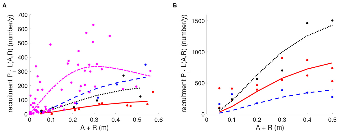
Figure 5. Statistical fitting of the larval production P and recruitment function L(A, R). For each site i, yearly recruitment P_iL(A, R) is shown. (A) Reefs with live adults A and dead shell R present; (B) Reefs with only dead shell R present and where A = 0. Red: Great Wicomico River sites GWR1 and GWR2; Purple: GWR3; Blue: Linkhorn Bay site, LB; Black: Broad Bay site, BB. Parameter values are in Tables 2, 3.

3.4. Carrying Capacity

We estimated carrying capacity K by assuming that mean SH = 100 mm for adult oysters (Schulte et al., 2009). Using the conversion function (Equation 8), the volume of an average adult oyster = 3.256 · 100^2.184 · 10⁻⁹ = 7.5977 · 10⁻⁵ m³. From field data, the maximum number of adult oysters in 1 m² averages 200 (Schulte et al., 2009). Including the packing parameter, K = 7.5977 · 10⁻⁵ · 4.6 · 200 = 0.06990 m³ · m⁻², which we rounded up to 0.1 as a maximum volume for K. We note that because K appears in the term of Equation (4) for positive change in biomass, it is not a carrying capacity in the traditional sense that populations will approach this value after a long time. Rather, it represents the population above which biomass cannot be generated.

3.5. Dead Oyster Shell Degradation Rate

For the dead oyster shell volume equation (Equation 5), the oyster shell degradation rate γ is estimated with the assumption that the average half life of oyster shell is 6 y (Powell et al., 2006). In the absence of live oysters, Equation (5) becomes a linear decay equation $\frac{dR}{dt}=-\gamma R$. Solving it with a half life of t = 6 y yields R(t) = R(0)e^−γt = R(0)/2, such that γ = ln(2)/6 = 0.1155 y⁻¹.

4. Results

4.1. Consistency of Single-Stage and Stage-Structured Models

Similar to the original model (Jordan-Cooley et al., 2011), the stage-structured JARS model possessed multiple equilibria. The extinction equilibrium E₀ = (0, 0, 0, C/β) always existed, and for most reasonable parameter values, it was locally asymptotically stable (see Appendix). This implies that for initial values close to the extinction state, the population would always go extinct. Moreover, persistence of the population occurred under similar values of C and initial conditions as in Jordan-Cooley et al. (2011). Below we document the regimes for parameters P (larval production) and C (water-column sediment deposition rate) that supported conditional persistence of the population, thus inducing alternative stable states. As with C, the parameter P was chosen due to its variability among oyster populations. When alternative stable states existed, we determined the initial conditions that led to persistence or extinction. While our results may also be applicable to a wider range of parameter values, we used the parameter values in Table 2 because they are based on previous studies, field data, and our estimates from fitting field data for restoration reefs.

4.2. Bifurcation Analysis

The effects of parameters P and C on the oyster population were examined through bifurcation analysis to determine four-dimensional (J, A, R, S) equilibrium population sizes as a function of the bifurcation parameters P and C. Bifurcation analysis employs bifurcation theory in non-linear dynamical systems (Kuznetsov, 1998) to produce a comprehensive evaluation of population dynamics. In population models, bifurcation analysis can detect ecological steady states as a function of model parameters and bifurcation points where dynamics change drastically (de Roos, 2021). Bifurcation diagrams were generated by Matlab package Matcont (Dhooge et al., 2003).

A bifurcation diagram with respect to larval production P is shown in Figure 6. In this and subsequent bifurcation diagrams, equilibrium population sizes (solid stable and dashed unstable curves) are depicted as a function of specific bifurcation parameters. Each bifurcation diagram also displays a saddle-node bifurcation point (LP) that represents the boundary between alternative stable states and population extinction (i.e., the tipping point). For instance, in Figure 6, P is the bifurcation parameter, such that for each value of P, equilibrium population sizes are indicated by the curves. The equilibria are four-dimensional (J, A, R, S), so we display each of the variables separately for clarity. Resilience is defined as the ability of a population to recover from a disturbance that reduces population abundance significantly. In Figure 6 and other bifurcation diagrams, resilience is proportional to the distance between the stable and unstable positive equilibria (Scheffer and Carpenter, 2003).

FIGURE 6

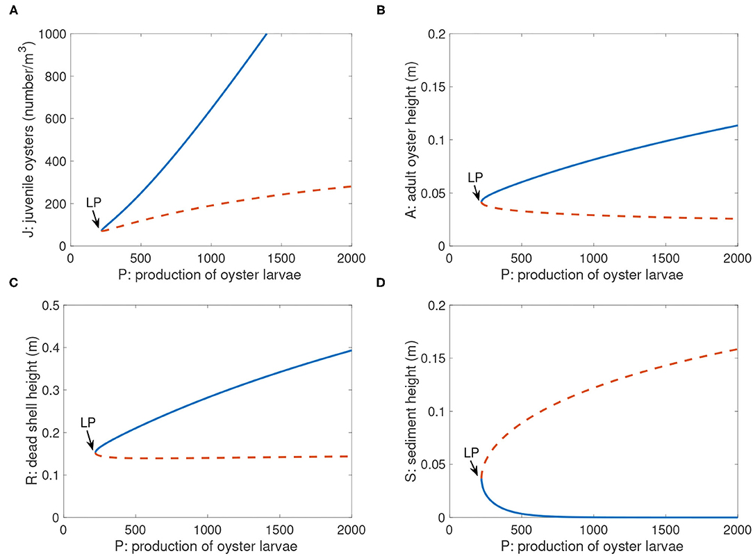
Figure 6. Bifurcation diagram of positive equilibria of Equations (1) and (4)-(6) with parameter P. Not shown is the extinction equilibrium line for J, A, and R, which is at the abscissa for all values of P. Parameter values are in Table 2. (A): J; (B): A; (C): R; (D): S. The point labeled “LP” is the saddle-node bifurcation point P_critical = 220.6. Blue solid branch: stable; orange dashed branch: unstable. The bifurcation diagram was generated by Matlab package Matcont.

4.3. Bifurcation Structure as a Function of P

The parameter P in Equation (1) represents the rate of larval production, and scales the larval recruitment function L(A, R). For P there was a threshold value P_critical = 220.6 such that when P < P_critical, there was no equilibrium with a positive population size (Figure 6); i.e., insufficient numbers of larvae were available to settle either from the natal population or from outside populations. All positive initial conditions approached an extinct state with zero population and high sediment level (not shown in the graphs). When P > P_critical, the system had two positive equilibria (Figure 6). The upper equilibrium (solid blue curve) represented stable high population sizes to which sufficiently large initial population sizes were attracted. The lower equilibrium (dashed orange curve) was an unstable smaller population representing a threshold below which populations went to extinction; above it populations moved toward the stable positive equilibrium (blue curve). Also, resilience increased proportional to larval production P (Figure 6), as reflected in the greater distances between stable solid blue and unstable dashed orange curves at high P.

P(i) values obtained through fitting field data in Table 3 were all above this threshold value P_critical = 220.6, except that P(2) was below. For P = 250, which will be used later as a benchmark point, there were two positive equilibrium states: (J, A, R, S) = (93.41, 0.05, 0.16, 0.02), which is locally asymptotically stable, and (J, A, R, S) = (73.8, 0.04, 0.15, 0.05), which is unstable. Similar bifurcation structure resulted when we used different parameter values in the analysis.

4.4. Bifurcation Structure as a Function of C and P

In our original single-stage model (Jordan-Cooley et al., 2011), the bifurcation structure of positive steady states of the model was explored in terms of maximum sediment deposition rate C. The bifurcation structure with parameter C was preserved in the JARS model (Figure 7). There was a threshold value C_critical, which depended on P, such that when C < C_critical, the system had two positive equilibria and resilience of J, A, and R increased as C decreased (Figure 7). When C > C_critical, there was no positive equilibrium; the extinction state attracted all initial values (Figure 7). The effect of the larval production rate P on bifurcation structure of C was to shift the saddle-node bifurcation point and positive equilibrium curves; larger values of P allowed the population to persist at higher values of C and increased resilience. For example, at P = 250, C_critical = 0.0225 (Figures 7A–D), whereas at P = 800, C_critical = 0.070 (Figures 7E–H). This level of larval production P = 800 is within the observed range of values in Chesapeake Bay (Schulte et al., 2009; Lipcius et al., 2015; Colden et al., 2017). The structure of the reef (values of J, A, and R) was insensitive to the sediment deposition rate C as long as C was below the bifurcation point (Figure 7). In contrast, the reef structure depended strongly on the larval production rate P.

FIGURE 7

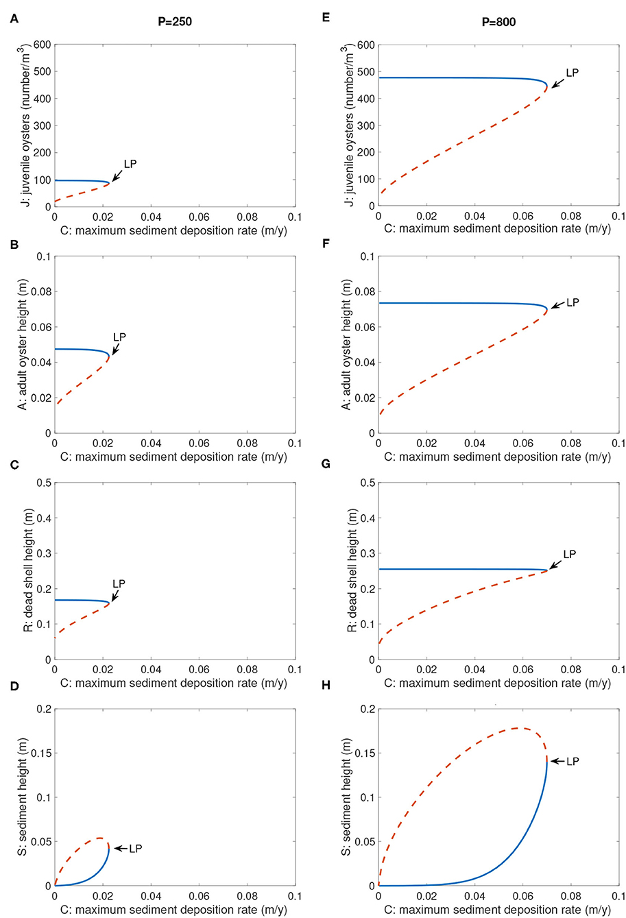
Figure 7. Bifurcation diagrams of positive equilibria for parameter C. (A–D) P = 250, (E–H) P = 800. Not shown is the extinction equilibrium line for J, A, and R, which is at the abscissa for all values of C and P. Other parameters are as in Table 2. Blue solid branch: stable; orange dashed branch: unstable.

Investigating the joint effects of P and C upon bifurcation structure also allowed us to obtain an estimate for the instantaneous growth rate of adult oysters ϕ. The threshold production rate of oyster larvae P for positive population states to exist was a function of maximum sediment deposition rate C (blue curve in Figure 9). To prevent local extinction and assure a positive equilibrium state, higher levels of P were required at higher concentrations of C to overcome the negative effects of sediment accumulation on the reef. Even at low maximum sediment deposition rates C, the larval production rate P had to be positive for populations to persist because the production of oyster larvae was the only source of new recruits in the model. Hence, we chose the instantaneous growth rate of adult oysters ϕ in Table 2 to reflect this requirement.

Although slightly non-linear, the location of the saddle-node bifurcation point (blue curve in Figure 9) was well-approximated by P = 11, 205C. For this set of environmental conditions, this provided a criterion for oyster restoration: If P > 11, 205C at a location, it would be possible to build a persisting oyster reef.

4.5. Threshold Reef Height

For application of the JARS model to oyster restoration, we determined critical values of R₀, initial reef height of dead oyster shell, to construct a reef for successful restoration. Threshold R₀ values were computed numerically, assuming the parameter values in Table 2. When S₀ = 0, there is initially no sediment on the restoration reef (Figure 8). As an illustration of the numerical analysis used to determine threshold reef height R₀, in Figure 8 we chose larval availability P to be 250, which is a scenario with sustainable dynamics (above P_critical = 220.6). When R₀ = 0.26 m the population persisted (Figure 8A), whereas when R₀ = 0.25 m the population declined to extinction (Figure 8B). Thus, the critical value should be between 0.25 and 0.26 m. The calculated critical value for R₀ was approximately R_0c = 0.253. In general and for other values of P, when R₀ ≥ R_0c (Figure 8A), the oyster population and reef persisted (Figure 8A). After some time, it approached the stable positive state. Otherwise, sediment S accumulated rapidly and the system moved toward an extinct state (Figure 8B).

FIGURE 8

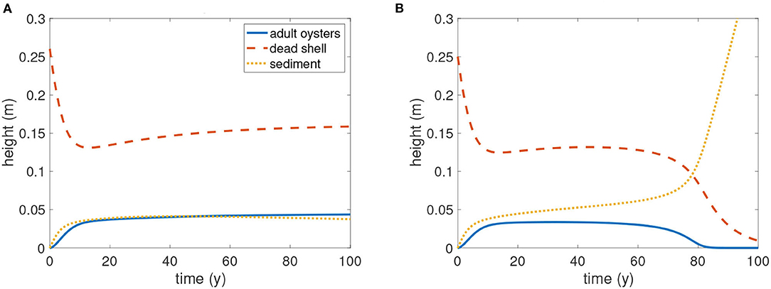
Figure 8. Determination of threshold reef height R₀ with P = 250, as an illustration of the numerical approach used for a range of values of P. In this example, the time series of solutions is plotted with initial condition (J, A, R, S) = (0, 0, R₀, 0). (A) R₀ = 0.26, non-extinct outcome; (B) R₀ = 0.25, extinct outcome. The threshold reef height R₀ is therefore between 0.25 and 0.26. Blue: adult oysters; red: dead oyster shells; yellow: sediment. Here P = 250 and other parameters are as in Table 2.

We also evaluated the joint influence of maximum sediment deposition rate C and production of oyster larvae P on R_0c (Figure 9) because these two parameters can differ substantially between locations (Cronin et al., 2003; Lipcius et al., 2015; Colden et al., 2017). The main result from this simulation was that at a given level of sediment deposition rate C, there existed a wide range of R_0c depending on larval availability P. The higher the P, the lower the initial reef height needed for any level of C (Figure 9). For instance, at a maximum sediment deposition rate C = 0.02 and P = 250, the initial dead shell reef height R₀ needed for persistence was about 0.253 m, whereas with P = 1,000, R_0c = 0.128 m, which is half that needed for P = 250. However, at each level of P there existed a bifurcation point C_critical such that at values of C above C_critical the population moved toward extinction irrespective of R₀ (Figure 9). The results of Figure 9 were robust to different values for maturation rate m and different parameters in the larval recruitment function L(A, R) obtained from fitting the recruitment data with and without GWR3 data.

FIGURE 9

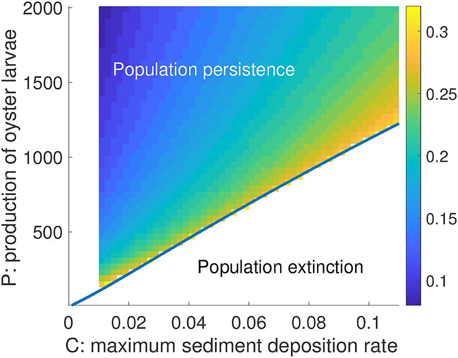
Figure 9. Critical reef height R_0c as a function of C and P in a 2-d color gradient representation. Blue curve is a superimposed bifurcation curve showing the saddle-node bifurcation point with respect to the joint effects of parameters C and P. Non-extinct outcomes exist only above the curve (including in the region of very small sediment deposition rates where R_0c was not computed). Other parameters are as in Table 2. The vertical bar legend to the right of the graph represents a gradient of R₀ in m.

For oyster restoration, we also focused on defining critical values of R₀, initial reef height of dead oyster shell, given different values of S₀, the initial height of sediment on a reef before larval settlement and recruitment occur (Figure 10). Under this scenario, restoration reefs are constructed with shell but without live oysters. Differing values of S₀ are applicable when restoration reefs are constructed at different time periods prior to settlement and recruitment, and sediment deposition C results in accumulation of sediment S on the reef. In Figure 10A, we used the lowest possible value for larval influx P = 221 for which reefs would persist. In this case the initial dead shell reef height R₀ necessary for persistence increased rapidly from under 0.3 m at S₀ = 0 to nearly 0.4 m at S₀ = 0.03 m. At higher levels of larval influx, such as P = 1, 000 (Figure 10B), the critical reef height dropped significantly; e.g., at S₀ = 0 critical reef height was less than 0.13 m for P = 1, 000, which was less than half the 0.3 m needed for P = 221 (Figure 10). For all levels of P, critical reef height increased with initial sediment. Especially when larval supply was poor, much higher initial reef heights R₀ were required for persistence to counteract the effect of sediment buildup on the reef before settlement occurred, as the initial sediment volume S₀ was amplified (Figure 10).

FIGURE 10

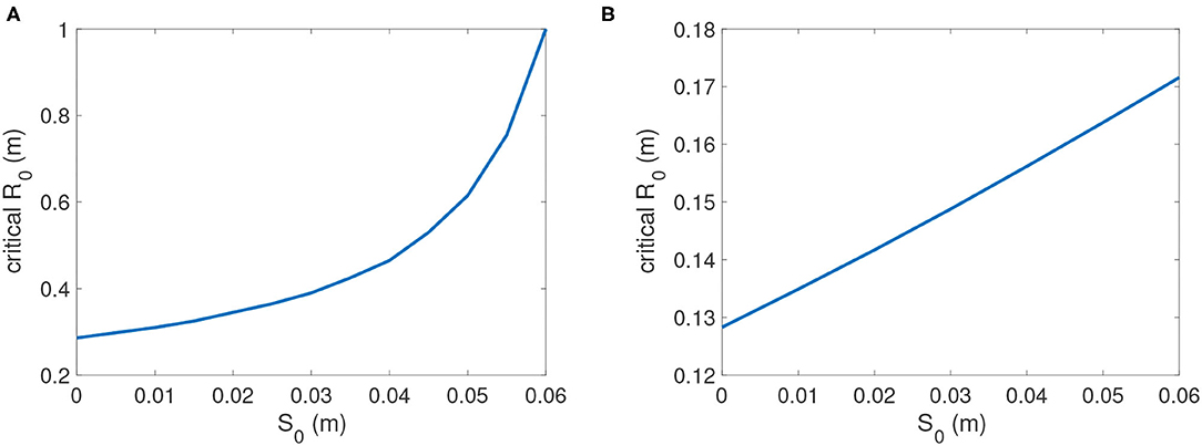
Figure 10. Critical reef height R_0c as a function of initial sediment height S₀. (A) P = 221; (B) P = 1, 000. Other parameters are as in Table 2.

5. Discussion

A stage-structured model composed of juvenile density J, and volumes of adults A (i.e., surrogate for biomass), dead oyster shell reef R, and sediment S on an oyster reef (JARS model) was parameterized with empirical data from field experiments. This enabled us to determine the collective influence of larval supply P and sediment deposition C on oyster reef resilience, and the critical initial dead-shell reef height R₀ for reef persistence. Larval supply was assumed to include the collective supply from the natal population and from larval subsidies from outside populations. Resilience was defined as by Scheffer and Carpenter (2003), specifically the ability of the oyster reef population to recover from disturbances that significantly reduce population abundance.

Similar to the single-stage model (Jordan-Cooley et al., 2011), the stage-structured JARS model possessed multiple equilibria (i.e., alternative stable states), such that different initial conditions of dead-shell reef height produced different final states. The main novel findings from the JARS model were that the critical initial reef height R₀ for population persistence was dependent not only on sediment input C, as in Jordan-Cooley et al. (2011), but also crucially on larval supply P and on S₀, the amount of sediment built up on a reef before settlement and recruitment of oysters. As larval influx P to a reef increased, the initial reef height R₀ needed for reef persistence was lower and oyster reef resilience was enhanced, such that an oyster reef with higher larval influx could recover from more severe disturbances than a reef with lower larval influx. In addition, a threshold larval supply P was identifiable, below which a shell reef could not survive. These results are consistent with field experiments using high- and low-relief reefs; the critical reef heights determined here were in the same range (0.15–0.30 m) as those in field experiments where reef height, larval recruitment and sediment concentration varied (Schulte et al., 2009; Lipcius et al., 2015; Colden et al., 2017). The effects of the magnitude of larval supply P on the impact of other parameters was to lower the magnitude of positive parameters, such as the instantaneous growth rate of adult oysters ϕ, required for population persistence. For example, larger values of P allowed the population to persist at lower values of ϕ and at higher values of negative parameters such as sediment concentration C, by increasing population resilience to disturbance.

These findings are valuable for our understanding not only of the ecology of oyster populations, but especially for oyster reef restoration because they can guide reef construction and placement to be effective and cost-efficient. When R₀ was greater than the threshold value of R, the oyster population and reef persisted. Otherwise, sediment S accumulated rapidly and the reef degraded to extinction. For larger values of P, the critical reef height decreased at most sediment concentrations. For instance, the critical reef height with no sediment at P = 300 was 20% lower than that with P = 221, which could reduce restoration costs significantly. This would be the situation when restoration reefs are constructed only out of dead shell R with no adults A₀ = 0 and immediately before the settlement and recruitment season such that S₀ = 0. In contrast, if reefs are constructed well before the settlement and recruitment period, and sediment S is allowed to build up on a reef before settlement and recruitment, then the relationship between R₀ and S₀ becomes critical in defining the additional initial dead shell reef height R₀ necessary for reef persistence. In our analyses, the critical R₀ was positively related to S₀ such that much higher initial reef heights R₀ were needed for reef persistence when the initial sediment volume S₀ on a reef was substantially greater than 0.

The characteristics of the interactions observed in the JARS model are highly relevant for marine species exhibiting metapopulation source-sink dynamics, which are common in marine and estuarine ecosystems (Lipcius and Ralph, 2011). For instance, the Lynnhaven River in lower Chesapeake Bay harbors an oyster metapopulation consisting of populations in interconnected bays and tributaries (Lipcius et al., 2015). Connectivity among the populations, as determined by biophysical modeling with historical oyster reef information, was complex and indicative of metapopulation structure (Lipcius et al., 2015). The metapopulation was apparently composed of four types of reef subpopulations with different implications for larval exchange and consequences for restoration strategies. Source subpopulation reefs were capable of self-replenishment and were interconnected with many of the reefs in the subestuary via larval exchange, indicating that these reefs were not only self-replenishing but also supplied larval subsidies to other reefs. These reefs are optimal for habitat restoration R and broodstock A enhancement, especially where no oyster population exists and the metapopulation must be jump-started with new source subpopulations. In contrast, sink subpopulation reefs did not self-replenish and larvae from sink reefs were advected out of the system, which makes these reefs unsuitable for broodstock A enhancement. However, sink reefs are suitable for habitat R restoration because these reefs would receive larval subsidies from source reefs once the source subpopulation reefs become established. Other self-replenishing subpopulation reefs supplied adequate larvae back to the natal reef, but did not supply larvae to other reefs in the system. Although such reefs are acceptable for habitat restoration and broodstock enhancement, they are, however, suboptimal in that their value to the metapopulation is limited. Finally, putative source subpopulation reefs alternated between self-replenishment and provision of larvae to other reefs, depending on environmental conditions. These reefs are thus acceptable for restoration and broodstock enhancement, but only after source subpopulation reefs have been restored.

The implications of our model for restoration are consistent with field experiments using high- and low-relief reefs, and the critical reef height determined here was very close to the field results (Schulte et al., 2009; Lipcius et al., 2015; Colden et al., 2017). However, initial conditions could vary from one site to another, and reliable estimates of parameters such as larval supply and sediment deposition rate are needed to determine the corresponding critical reef heights. In addition, habitat quality must be incorporated through habitat suitability index models (Theuerkauf and Lipcius, 2016) to define the optimal restoration strategy. By taking into account oyster juveniles as well as larval recruitment, our JARS model incorporates the age structure of oyster populations and thus provides a better conceptual framework for real-world oyster restoration.

Future refinements of the model should include time-varying parameters. For instance, larval supply P is actually time varying due to the effects of salinity and hydrodynamic changes resulting from freshwater discharge and rainfall, so fluctuations in P should be investigated. Also, we didn't model the effect of non-zero initial adult oysters A on critical reef R height, which may be significant due to the filtering ability and reproductive output of adult oysters (Wilson, 2019). Furthermore, larval supply P could be separated into natal and outside components to reflect the likely different contributions of outside and natal populations to reef persistence. Such modifications could be effectively modeled using the JARS model system.

Data Availability Statement

The original contributions presented in the study are included in the article/Supplementary Material, further inquiries can be directed to the corresponding author/s.

Author Contributions

RL provided field data used to parameterize the model and produced the function of oyster biomass vs. size. YZ, JZ, LS, and JS analyzed the model. RL, YZ, LS, and JS wrote the manuscript. All authors developed the model.

Funding

Funding was provided through research grants to LS, JS, and RL by the National Science Foundation's Division of Mathematical Sciences program in Mathematical Biology (DMS-1313243, DMS-1313093, and DMS-1715651) and EXTREEMS-QED program (DMS-1331021), and to RL by the National Oceanic and Atmospheric Administration's Chesapeake Bay Office program in Oyster Restoration Ecosystem Services.

Conflict of Interest

The authors declare that the research was conducted in the absence of any commercial or financial relationships that could be construed as a potential conflict of interest.

Publisher's Note

All claims expressed in this article are solely those of the authors and do not necessarily represent those of their affiliated organizations, or those of the publisher, the editors and the reviewers. Any product that may be evaluated in this article, or claim that may be made by its manufacturer, is not guaranteed or endorsed by the publisher.

Acknowledgments

This is contribution number 4049 of the Virginia Institute of Marine Science, William and Mary.

Supplementary Material

The Supplementary Material for this article can be found online at: https://www.frontiersin.org/articles/10.3389/fmars.2021.677640/full#supplementary-material

Footnotes

1. ^Ducharme-Barth, N., Lipcius, R. N., Shaw, L. B., and Shi, J. (2021). Reef degradation due to exploitation triggers population collapse and lowers MSY of oyster populations.

References

Airoldi, L., and Beck, M. (2007). Loss, status and trends for coastal marine habitats of Europe. Oceanogr. Mar. Biol. Annu. Rev. 45, 345–405. doi: 10.1201/9781420050943.ch7

CrossRef Full Text | Google Scholar

Baylor, J. B. (1895). Complete Survey of the Natural Oyster Beds, Rocks, and Shoals of Virginia. Report to the Governor of Virginia. US Superintendent of Public Printing.

Beck, M. W., Brumbaugh, R. D., Airoldi, L., Carranza, A., Coen, L. D., Crawford, C., et al. (2011). Oyster reefs at risk and recommendations for conservation, restoration, and management. Bioscience 61, 107–116. doi: 10.1525/bio.2011.61.2.5

CrossRef Full Text | Google Scholar

Cerco, C., and Noel, M. (2007). Can oyster restoration reverse cultural eutrophication in Chesapeake Bay? Estuar. Coasts 30, 331–343. doi: 10.1007/BF02700175

CrossRef Full Text | Google Scholar

Coen, L. D., Brumbaugh, R. D., Bushek, D., Grizzle, R., Luckenbach, M. W., Posey, M. H., et al. (2007). Ecosystem services related to oyster restoration. Mar. Ecol. Prog. Ser. 341, 303–307. doi: 10.3354/meps341303

CrossRef Full Text | Google Scholar

Colden, A. M., Fall, K. A., Cartwright, G. M., and Friedrichs, C. T. (2016). Sediment suspension and deposition across restored oyster reefs of varying orientation to flow: implications for restoration. Estuar. Coasts 39, 1435–1448. doi: 10.1007/s12237-016-0096-y

CrossRef Full Text | Google Scholar

Colden, A. M., Latour, R. J., and Lipcius, R. N. (2017). Reef height drives threshold dynamics of restored oyster reefs. Mar. Ecol. Prog. Ser. 582, 1–13. doi: 10.3354/meps12362

CrossRef Full Text | Google Scholar

Colden, A. M., and Lipcius, R. N. (2015). Lethal and sublethal effects of sediment burial on the eastern oyster Crassostrea virginica. Mar. Ecol. Prog. Ser. 527, 105–117. doi: 10.3354/meps11244

CrossRef Full Text | Google Scholar

Connolly, S. R., and Roughgarden, J. (1999). Theory of marine communities: competition, predation, and recruitment-dependent interaction strength. Ecol. Monogr. 69, 277–296. doi: 10.1890/0012-9615(1999)069[0277:TOMCCP]2.0.CO;2

CrossRef Full Text | Google Scholar

Cronin, T., Sanford, L., Langland, M., Willard, D., and Saenger, C. (2003). “Estuarine sediment transport, deposition, and sedimentation,” in A Summary Report of Sediment Processes in Chesapeake Bay and Watershed, Water-Resources Investigations Report 03-4123, eds M. Langland and T. Cronin (Gloucester Point, VA: Virginia Institute of Marine Science, College of William and Mary), 61–79.

de Roos, A. M. (2021). Pspmanalysis: steady-state and bifurcation analysis of physiologically structured population models. Methods Ecol. Evol. 12, 383–390. doi: 10.1111/2041-210X.13527

CrossRef Full Text | Google Scholar

Dekshenieks, M., Hofmann, E., Klinck, J., and Powell, E. (1996). Modeling the vertical distribution of oyster larvae in response to environmental conditions. Mar. Ecol. Prog. Ser. 136, 97–110. doi: 10.3354/meps136097

CrossRef Full Text | Google Scholar

Dekshenieks, M. M., Hofmann, E. E., and Powell, E. N. (1993). Environmental effects on the growth and development of eastern oyster, Crassostrea virginica (Gmelin, 1791), larvae: a modeling study. J. Shellfish Res. 12, 241–254.

Google Scholar

DePiper, G. S., Lipton, D. W., and Lipcius, R. N. (2017). Valuing ecosystem services: oysters, denitrification, and nutrient trading programs. Mar. Resour. Econ. 32, 1–20. doi: 10.1086/688976

CrossRef Full Text | Google Scholar

Dhooge, A., Govaerts, W., and Kuznetsov, Y. A. (2003). MATCONT: a Matlab package for numerical bifurcation analysis of ODEs. ACM Trans. Math. Softw. 29, 141–164. doi: 10.1145/779359.779362

CrossRef Full Text | Google Scholar

Doering, K. L., Wilberg, M. J., Liang, D., and Tarnowski, M. (2021). Patterns in oyster natural mortality in Chesapeake Bay, Maryland using a Bayesian model. Fish. Res. 236:105838. doi: 10.1016/j.fishres.2020.105838

CrossRef Full Text | Google Scholar

Edmunds, P. J., and Riegl, B. (2020). Urgent need for coral demography in a world where corals are disappearing. Mar. Ecol. Prog. Ser. 635, 233–242. doi: 10.3354/meps13205

CrossRef Full Text | Google Scholar

Grabowski, J., and Peterson, C. (2007). “Restoring oyster reefs to recover ecosystem services,” in Ecosystem Engineers, eds K. Cuddington, J. Byers, W. Wilson, and A. Hastings (Cambridge, UK: Academic Press), 281–298. doi: 10.1016/S1875-306X(07)80017-7

CrossRef Full Text | Google Scholar

Grabowski, J. H., Brumbaugh, R. D., Conrad, R. F., Keeler, A. G., Opaluch, J. J., Peterson, C. H., et al. (2012). Economic valuation of ecosystem services provided by oyster reefs. Bioscience 62, 900–909. doi: 10.1525/bio.2012.62.10.10

CrossRef Full Text | Google Scholar

Hofmann, E., Powell, E., Bochenek, E., and Klinck, J. (2004). A modelling study of the influence of environment and food supply on survival of Crassostrea gigas larvae. ICES J. Mar. Sci. 61, 596–616. doi: 10.1016/j.icesjms.2004.03.029

CrossRef Full Text | Google Scholar

Hofmann, E. E., Klinck, J. M., Powell, E. N., Boyles, S., and Ellis, M. (1994). Modeling oyster populations II. Adult size and reproductive effort. J. Shellfish Res. 13, 165–182.

Google Scholar

Hofmann, E. E., Powell, E. N., Klinck, J. M., and Wilson, E. A. (1992). Modeling oyster populations III. Critical feeding periods, growth and reproduction. J. Shellfish Res. 11, 399–416.

Google Scholar

Housego, R. M., and Rosman, J. H. (2016). A model for understanding the effects of sediment dynamics on oyster reef development. Estuar. Coasts 39, 495–509. doi: 10.1007/s12237-015-9998-3

CrossRef Full Text | Google Scholar

Jackson, J. B., Kirby, M. X., Berger, W. H., Bjorndal, K. A., Botsford, L. W., Bourque, B. J., et al. (2001). Historical overfishing and the recent collapse of coastal ecosystems. Science 293, 629–637. doi: 10.1126/science.1059199

PubMed Abstract | CrossRef Full Text | Google Scholar

Jordan, S. (1987). Sedimentation and remineralization associated with biodeposition by the American oyster Crassostrea virginica (Gmelin) (Ph.D. thesis). University of Maryland, College Park, MD, United States.

Google Scholar

Jordan-Cooley, W. C., Lipcius, R. N., Shaw, L. B., Shen, J., and Shi, J. (2011). Bistability in a differential equation model of oyster reef height and sediment accumulation. J. Theoret. Biol. 289, 1–11. doi: 10.1016/j.jtbi.2011.08.013

PubMed Abstract | CrossRef Full Text | Google Scholar

Kennedy, V., Breitburg, D., Christman, M., Luckenbach, M., Paynter, K., Kramer, J., et al. (2011). Lessons learned from efforts to restore oyster populations in Maryland and Virginia, 1990 to 2007. J. Shellfish Res. 30, 719–731. doi: 10.2983/035.030.0312

CrossRef Full Text | Google Scholar

Kirby, M. X. (2004). Fishing down the coast: historical expansion and collapse of oyster fisheries along continental margins. Proc. Natl. Acad. Sci. U.S.A. 101, 13096–13099. doi: 10.1073/pnas.0405150101

PubMed Abstract | CrossRef Full Text | Google Scholar

Klinck, J. M., Hofmann, E. E., Powell, E. N., and Dekshenieks, M. M. (2002). Impact of channelization on oyster production: a hydrodynamic-oyster population model for Galveston Bay, Texas. Environ. Model. Assess. 7, 273–289. doi: 10.1023/A:1020954502355

CrossRef Full Text | Google Scholar

Kniskern, T., and Kuehl, S. (2003). Spatial and temporal variability of seabed disturbance in the York River subestuary. Estuar. Coast. Shelf Sci. 58, 37–55. doi: 10.1016/S0272-7714(03)00052-0

CrossRef Full Text | Google Scholar

Kuznetsov, Y. A. (1998). Elements of applied bifurcation theory. Second edition. Applied Mathematical Sciences, 112. New York, NY: Springer-Verlag.

Google Scholar

La Peyre, M., Furlong, J., Brown, L. A., Piazza, B. P., and Brown, K. (2014). Oyster reef restoration in the northern Gulf of Mexico: Extent, methods and outcomes. Ocean Coast. Manage. 89, 20–28. doi: 10.1016/j.ocecoaman.2013.12.002

CrossRef Full Text | Google Scholar

Lavaud, R., La Peyre, M. K., Casas, S. M., Bacher, C., and La Peyre, J. F. (2017). Integrating the effects of salinity on the physiology of the eastern oyster, Crassostrea virginica, in the northern Gulf of Mexico through a Dynamic Energy Budget model. Ecol. Modell. 363, 221–233. doi: 10.1016/j.ecolmodel.2017.09.003

CrossRef Full Text | Google Scholar

Lipcius, R., and Ralph, G. (2011). “Evidence of source-sink dynamics in marine and estuarine species,” in Sources, Sinks and Sustainability, eds J. Liu, V. Hull, A. Morzillo, and J. Wiens (Cambridge: Cambridge University Press), 361–381. doi: 10.1017/CBO9780511842399.019

CrossRef Full Text | Google Scholar

Lipcius, R. N., and Burke, R. P. (2018). Successful recruitment, survival and long-term persistence of eastern oyster and hooked mussel on a subtidal, artificial restoration reef system in Chesapeake Bay. PLoS ONE 13:e0204329. doi: 10.1371/journal.pone.0204329

PubMed Abstract | CrossRef Full Text | Google Scholar

Lipcius, R. N., Burke, R. P., McCulloch, D. N., Schreiber, S. J., Schulte, D. M., Seitz, R. D., et al. (2015). Overcoming restoration paradigms: value of the historical record and metapopulation dynamics in native oyster restoration. Front. Mar. Sci. 2:65. doi: 10.3389/fmars.2015.00065

CrossRef Full Text | Google Scholar

Lipcius, R. N., Eggleston, D. B., Fodrie, F. J., Van Der Meer, J., Rose, K. A., Vasconcelos, R. P., et al. (2019). Modeling quantitative value of habitats for marine and estuarine populations. Front. Mar. Sci. 6:280. doi: 10.3389/fmars.2019.00280

CrossRef Full Text | Google Scholar

Lotze, H. K., Lenihan, H. S., Bourque, B. J., Bradbury, R. H., Cooke, R. G., Kay, M. C., et al. (2006). Depletion, degradation, and recovery potential of estuaries and coastal seas. Science 312, 1806–1809. doi: 10.1126/science.1128035

PubMed Abstract | CrossRef Full Text | Google Scholar

Moore, J. L., Lipcius, R. N., Puckett, B., and Schreiber, S. J. (2016). The demographic consequences of growing older and bigger in oyster populations. Ecol. Appl. 26, 2206–2217. doi: 10.1002/eap.1374

PubMed Abstract | CrossRef Full Text | Google Scholar

Moore, J. L., Puckett, B. J., and Schreiber, S. J. (2018). Restoration of eastern oyster populations with positive density dependence. Ecol. Appl. 28, 897–909. doi: 10.1002/eap.1694

PubMed Abstract | CrossRef Full Text | Google Scholar

Pace, S. M., Poussard, L. M., Powell, E. N., Ashton-Alcox, K. A., Kuykendall, K. M., Solinger, L. K., et al. (2020). Dying, decaying, and dissolving into irrelevance: first direct in-the-field estimate of Crassostrea virginica shell loss–a case history from Mississippi Sound. J. Shellfish Res. 39, 245–256. doi: 10.2983/035.039.0206

CrossRef Full Text | Google Scholar

Pine, W. E. III., Walters, C. J., Camp, E. V., Bouchillon, R., Ahrens, R., et al. (2015). The curious case of eastern oyster Crassostrea virginica stock status in Apalachicola Bay, Florida. Ecol. Soc. 20. doi: 10.5751/ES-07827-200346

CrossRef Full Text | Google Scholar

Powell, E., Kraeuter, J., and Ashton-Alcox, K. (2006). How long does oyster shell last on an oyster reef? Estuar. Coast. Shelf Sci. 69, 531–542. doi: 10.1016/j.ecss.2006.05.014

CrossRef Full Text | Google Scholar

Powell, E. N., Hofmann, E. E., and Klinck, J. M. (2018). Oysters, sustainability, management models, and the world of reference points. J. Shellfish Res. 37, 833–849. doi: 10.2983/035.037.0413

CrossRef Full Text | Google Scholar

Powell, E. N., Hofmann, E. E., Klinck, J. M., and Ray, S. M. (1992). Modeling oyster populations I. a commentary on filtration rate. Is faster always better? J. Shellfish Res. 11, 387–398.

Google Scholar

Powell, E. N., and Klinck, J. M. (2007). Is oyster shell a sustainable estuarine resource? J. Shellfish Res. 26, 181–194.

Google Scholar

Powell, E. N., Klinck, J. M., Ashton-Alcox, K., Hofmann, E. E., and Morson, J. (2012). The rise and fall of Crassostrea virginica oyster reefs: the role of disease and fishing in their demise and a vignette on their management. J. Mar. Res. 70, 505–558. doi: 10.1357/002224012802851878

CrossRef Full Text | Google Scholar

Powell, E. N., Klinck, J. M., Ashton-Alcox, K. A., and Kraeuter, J. N. (2009). Multiple stable reference points in oyster populations: biological relationships for the eastern oyster (Crassostrea virginica) in Delaware Bay. U.S. Fish. Bull. 107, 109–132.

Google Scholar

Powell, E. N., Klinck, J. M., and Hofmann, E. E. (2011). Generation time and the stability of sex-determining alleles in oyster populations as deduced using a gene-based population dynamics model. J. Theoret. Biol. 271, 27–43. doi: 10.1016/j.jtbi.2010.11.006

PubMed Abstract | CrossRef Full Text | Google Scholar

Powell, E. N., Song, J., Ellis, M. S., and Wilson-Ormond, E. A. (1995). The status and long-term trends of oyster reefs in Galveston Bay, Texas. J. Shellfish Res. 14, 439–457.

Google Scholar

Powers, S. P., Peterson, C. H., Grabowski, J. H., Lenihan, H. S., et al. (2009). Success of constructed oyster reefs in no-harvest sanctuaries: implications for restoration. Mar. Ecol. Prog. Ser. 389, 159–170. doi: 10.3354/meps08164

CrossRef Full Text | Google Scholar

Puckett, B. J., and Eggleston, D. B. (2012). Oyster demographics in a network of no-take reserves: recruitment, growth, survival, and density dependence. Mar. Coast. Fish. 4, 605–627. doi: 10.1080/19425120.2012.713892

CrossRef Full Text | Google Scholar

Rothschild, B., Ault, J., Goulletquer, P., and Heral, M. (1994). Decline of the Chesapeake Bay oyster population: a century of habitat destruction and overfishing. Mar. Ecol. Prog. Ser. 111, 29–39. doi: 10.3354/meps111029

CrossRef Full Text | Google Scholar

Scheffer, M., and Carpenter, S. R. (2003). Catastrophic regime shifts in ecosystems: linking theory to observation. Trends Ecol. Evol. 18, 648–656. doi: 10.1016/j.tree.2003.09.002

CrossRef Full Text | Google Scholar

Schulte, D. M. (2017). History of the Virginia oyster fishery, Chesapeake Bay, USA. Front. Mar. Sci. 4:127. doi: 10.3389/fmars.2017.00127

CrossRef Full Text | Google Scholar

Schulte, D. M., Burke, R. P., and Lipcius, R. N. (2009). Unprecedented restoration of a native oyster metapopulation. Science 325, 1124–1128. doi: 10.1126/science.1176516

PubMed Abstract | CrossRef Full Text | Google Scholar

Smith, G. F., Bruce, D. G., Roach, E. B., Hansen, A., Newell, R. I. E., and McManus, A. M. (2005). Assessment of recent habitat conditions of eastern oyster Crassostrea virginica bars in mesohaline Chesapeake Bay. North Am. J. Fish. Manage.25, 1569–1590. doi: 10.1577/M04-058.1

CrossRef Full Text | Google Scholar

Soniat, T. M., Cooper, N., Powell, E. N., Klinck, J. M., Abdelguerfi, M., Tu, S., et al. (2014). Estimating sustainable harvests of eastern oysters, Crassostrea virginica. J. Shellfish Res. 33, 381–394. doi: 10.2983/035.033.0207

CrossRef Full Text | Google Scholar

Taylor, J., and Bushek, D. (2008). Intertidal oyster reefs can persist and function in a temperate North American Atlantic estuary. Mar. Ecol. Prog. Ser. 361, 301–306. doi: 10.3354/meps07429

CrossRef Full Text | Google Scholar

Theuerkauf, S. J., and Lipcius, R. N. (2016). Quantitative validation of a habitat suitability index for oyster restoration. Front. Mar. Sci. 3:64. doi: 10.3389/fmars.2016.00064

CrossRef Full Text | Google Scholar

van Rijn, L. C. (1986). Sediment Transport by Currents and Waves. Delft Hydraulics, Report H461.

Google Scholar

Vølstad, J. H., Dew, J., and Tarnowski, M. (2008). Estimation of annual mortality rates for eastern oysters (Crassostrea virginica) in Chesapeake Bay based on box counts and application of those rates to project population growth of C. virginica and C. ariakensis. J. Shellfish Res. 27, 525–533. doi: 10.2983/0730-8000(2008)27[525:EOAMRF]2.0.CO;2

CrossRef Full Text | Google Scholar

Weber, E. D., Vølstad, J. H., Christman, M. C., Lewis, D., and Dew-Baxter, J. R. (2013). Application of a demographic model for evaluating proposed oyster-restoration actions in Chesapeake Bay. Hum. Ecol. Risk Assess. Int. J. 19, 1187–1203. doi: 10.1080/10807039.2013.767110

CrossRef Full Text | Google Scholar

Wilberg, M., Livings, M., Barkman, J., Morris, B., and Robinson, J. (2011). Overfishing, disease, habitat loss, and potential extirpation of oysters in upper Chesapeake Bay. Mar. Ecol. Prog. Ser. 436, 131–144. doi: 10.3354/meps09161

CrossRef Full Text | Google Scholar

Wilberg, M. J., Wiedenmann, J. R., and Robinson, J. M. (2013). Sustainable exploitation and management of autogenic ecosystem engineers: application to oysters in Chesapeake Bay. Ecol. Appl. 23, 766–776. doi: 10.1890/12-0563.1

PubMed Abstract | CrossRef Full Text | Google Scholar

Wilson, R. (2019). A stage-structured oyster population model for reef restoration (Undergraduate Honors thesis). William and Mary, Williamsburg, VA, United States.

Google Scholar

Winslow, F. (1881). Report on the Oyster Beds of the James River, Virginia, and of Tangier and Pocomoke Sounds, Maryland and Virginia. US Government Printing Office. Williamsburg, Virginia, USA.

Google Scholar

Yurek, S., Eaton, M. J., Lavaud, R., Laney, R. W., DeAngelis, D. L., Pine, I. I. I., et al. (2021). Modeling structural mechanics of oyster reef self-organization including environmental constraints and community interactions. Ecol. Modell. 440:109389. doi: 10.1016/j.ecolmodel.2020.109389

CrossRef Full Text | Google Scholar

Zu Ermgassen, P. S., Spalding, M. D., Blake, B., Coen, L. D., Dumbauld, B., Geiger, S., et al. (2012). Historical ecology with real numbers: past and present extent and biomass of an imperilled estuarine habitat. Proc. R. Soc. B Biol. Sci. 279, 3393–3400. doi: 10.1098/rspb.2012.0313

PubMed Abstract | CrossRef Full Text | Google Scholar