St Helena Marine Water Quality: Background Conditions and Development of Assessment Levels for Coastal Pollutants

St Helena is an isolated oceanic island located in the tropical South Atlantic, and knowledge of broadscale oceanography and productivity in its surrounding waters is limited. This study used model outputs (2007-2017), remote sensing data (1998-2017) and survey measurements (April 2018 and 2019) to determine background conditions for nutrients, chlorophyll and suspended particulate matter (SPM) in offshore waters and propose standards (thresholds) for assessing inshore water quality based on 50% deviation from seasonal (usually June to November) or annual averages. Seasonal thresholds were proposed for surface nitrate (average 0.18 μM), phosphate (average 0.26 μM), silicate (average 2.60 μM), chlorophyll (average 0.45 μg chl l^–1), and SPM (average 0.96 mg l^–1). Associated background values for most surface parameters (phosphate 0.17 μM, silicate 1.57 μM, chlorophyll 0.30 μg chl l^–1; from model outputs and remote sensing) were slightly higher than offshore observations (April 2019). For nitrate, the average background value (0.12 μM) was lower than the observed average (0.24 μM). At depth (150-500 m), annual background values from model outputs were high (nitrate 26.8 μM, phosphate 1.8 μM, silicate 17.3 μM). Observed water masses at depths >150 m, identified to be of Antarctic and Atlantic origin, were nutrient-rich (e.g., 16 μM for nitrate, April 2019) and oxygen deficient (<4-6 mg l^–1). A thermocline layer (between ca. 10 and 230 m), characterized by a sub-surface chlorophyll maximum (average 0.3-0.5 μg chl l^–1) near the bottom of the euphotic zone (ca. 100 m), is likely to sustain primary and secondary production at St Helena. For assessing inshore levels of chemical contaminants and fecal bacteria estimated from survey measurements, standards were derived from the literature. A preliminary assessment of inshore observations using proposed thresholds from surface offshore waters and relevant literature standards indicated concerns regarding levels of nutrients and fecal bacteria at some locations. More detailed modeling and/or field-based studies are required to investigate seasonal trends and nutrient availability to inshore primary producers and to establish accurate levels of any contaminants of interest or risk to the marine environment.

Introduction

St Helena is an isolated oceanic island, located in the tropical South Atlantic. The island provides habitat for a diverse range of tropical and sub-tropical marine species, many of which are endemic, CITES listed or listed on the IUCN Red List (IUCN, 2020). In September 2016, the 200 nm maritime zone or Exclusive Economic Zone (EEZ) around St Helena was declared an IUCN Category VI (Sustainable Use) Marine Protected Area (MPA) to provide protection for its biodiversity and to help ensure sustainable use of its natural resources.

St Helena is located approximately 1,500 km south of the equator, where warm surface waters contain few nutrients. To the south of the island, the surface waters of the subtropical gyre are also low in nutrients (McClain et al., 2004; Turner, 2020). Despite this, the marine waters around the island sustain productive commercial and recreational fisheries. Few (if any) field-based studies have been published on the physical, chemical and biological oceanography of the region. There is therefore limited information on how overall productivity in the marine waters around St Helena is sustained, and likely impacts of pressures such as climate change and ocean acidification. Marine production is likely to be influenced by broadscale oceanography, including the Benguela and Angola Currents (Feistel et al., 2003; Ellick et al., 2013; Cabos et al., 2017). Interactions between the atmosphere and the ocean influence winds, sea surface temperatures, currents, and resulting depths at which the nutrient-rich water is found. Studies from similar regions (e.g., Herbland et al., 1985) indicate that nutrients and plankton are generally found below the surface. Both mixing and upwelling are likely to play a key role in delivering nutrients into the surface waters. Eddy transport is also known to play a key role in westward transport of nutrients across the Atlantic subtropical gyres (McGillicuddy, 2016; Doddridge and Marshall, 2018).

Water quality plays a key role in determining the health of species and habitats within the marine environment. At St Helena, the main anthropogenic risks to marine water quality are directly from contaminants and marine debris from fishing, oil/chemical spills from shipping accidents, land-based run-off including untreated sewage (St Helena Government, 2016; Blue Belt Programme, 2018) and indirectly, through climate change. The on-island population is small (averaging 4,500 people since 2011; St Helena Government, 2018) and activities (e.g., boating, construction, provisioning) are largely related to fishing and a growing tourism industry (average visitor numbers per month since 2011 = 164; maximum 478 in December 2019¹). Most goods are imported as there is little agriculture or animal husbandry, and only fish and coffee are exported (St Helena Government, 2018). Wastewater from most properties is discharged through soakaways or septic tanks and management measures are underway to dispose of most sludge from a few settlements at a landfill site. A substantial amount of untreated sewage (and gray water) is discharged into the marine environment, for example at West Rocks (James Bay) and at Half Tree Hollow (St Helena Government, 2016), although there is a proposal for a wastewater scheme to screen effluent before discharging it offshore via a 500 m pipe (McVittie et al., 2019). Untreated sewage and storm water discharges may cause nutrient and microbiological contamination of the wider marine environment and marine biota. Bacteria, viruses and protozoans from human and animal sources, mainly attached to fine particulate matter, can affect bathing water quality and can accumulate in filter feeding shellfish (Potasman et al., 2002; OSPAR, 2009, 2010). A wide range of commonly used chemicals such as metals, herbicides and hydrocarbons may occur as contaminants in coastal and marine waters. Toxic contaminants generally alter marine ecosystem functioning by reducing productivity and increasing respiration (Johnston et al., 2015) and may have chronic effects on the growth and hatching rate of marine organisms (Law and Hii, 2006). Chemical pollutants such as pharmaceuticals and steroids may have endocrine disrupting effects on marine organisms (Smith et al., 2015).

Very little information is available on marine water quality at St Helena to support assessments of the state of the environment. Assessments usually require long term monitoring data and the development of standards or thresholds for key water quality parameters against which the data can be compared (e.g., Foden et al., 2011; OSPAR, 2013). Guidelines and standards have been developed in a number of regions, e.g., in South Africa, Europe, the United States, Australia and the Middle East (EIMP, 2001; EU, 2009, 2016; Brodie et al., 2011; DEA, 2012, 2018; Kress et al., 2019). Much of the guidance on the setting of standards or thresholds is based on establishing regional background concentrations using historical data and developing statistical measures, such as mean annual values or seasonal averages. Assessments of status can include analyses of long-term trends in the data in order to determine if observed changes are significant and in the direction required (e.g., EU, 2008a; COM, 2014). For example, for assessing anthropogenic nutrient enrichment and the impacts thereof (Tett et al., 2007), the direction required is generally downwards for nutrients and upwards for dissolved oxygen.

The aim of this study was to determine background environmental conditions and levels of pollutants (nutrients, chemical contaminants, and fecal indicator bacteria) in coastal waters at St Helena and to propose water quality standards (thresholds) for assessments of water quality. Data were obtained from model outputs and remote sensing, as well as measurements obtained during field surveys in 2018 and 2019. In 2019, samples were collected for analysis of nutrients (offshore and inshore), chlorophyll (offshore only), and chemical contaminants and fecal indicators (inshore only).

Methods

Model and Satellite Data

Physical oceanographic data were obtained from global ocean model output (EU Copernicus Marine Services Information, 2018a), at a resolution of 1/12 degree (equivalent to a grid spacing of approximately 9 km at 16°S). Monthly mean fields were obtained for the period 2007-2017, allowing seasonal climatology to be determined over this time. Supporting atmospheric data were obtained from the European Centre for Medium-Range Weather Forecasts (ECMWF) atmospheric reanalysis product, ERA5 (Hersbach et al., 2019). Monthly wind speeds were obtained for the period 2010-2017.

Resulting ocean and atmospheric data were analyzed for a region extending approximately 100 km offshore around St Helena. At the resolution of the oceanographic model (1/12 degree), St Helena island itself is not represented. However, the model does include shallower bathymetry at the island’s location, and hence potential impacts on circulation, upwelling and mixing. The point at which the model bathymetry is shallowest (16.0°S, 5.75°W) was then chosen to be representative of conditions around the island.

Nutrient data were obtained from a global biogeochemical model reanalysis (EU Copernicus Marine Services Information, 2018b), at a resolution of 1/4 degree (equivalent to a grid spacing of approximately 27 km at 16°S). Monthly mean fields were obtained for the period 2007-2016, allowing seasonal cycles and variability to be determined over this time. At the resolution of the model (1/4 degree), again St Helena island was not represented. The nearest point was then chosen to represent likely conditions in the region (16.0°S, 5.75°W). Model simulations did not include nutrient sources from the island itself (e.g., through river runoff).

Ocean color data were obtained from merged satellite remote sensing products. Concentrations of chlorophyll (chl) and suspended particulate matter (SPM) were extracted at a resolution of 1/24 degree, equivalent to approximately 4 km grid spacing, for the period 1998-2017. At the time of this study, this required use of two different products, using reprocessed data for 1998-2016, and near real time data for 2017 (EU Copernicus Marine Services Information, 2018c-f). Data were downloaded as monthly averages, for a region approximately 100 km offshore around St Helena. To identify seasonal trends in waters immediately surrounding St Helena, ocean color data were averaged monthly for a smaller region (ca 25 km × 25 km) around the island. This region was a rectangle covering 15.85-16.06°S and 5.85-5.60°W, comprising 7 × 6 grid points.

Background Environmental Conditions and Proposed Thresholds

Background environmental conditions for nutrients, chlorophyll and SPM were estimated from model and satellite data. Monthly averages in surface waters were plotted over a 10- or 20- year period to identify seasonal trends and estimate background conditions at St Helena for seasons with highest natural values, e.g., June to November, given as seasonal averages and maximum values. Proposed assessment levels (thresholds) were developed following an approach used in Europe to meet the needs of various directives (COM, 2003; OSPAR, 2005; Devlin et al., 2011; Foden et al., 2011). These approaches typically allow for 50% deviation from background conditions during the most relevant season, for example the phytoplankton growth season for chlorophyll and the preceding period with highest nutrient levels. The Redfield ratio of N:P (16:1) plus 50% deviation was used to calculate a threshold value (24) for the ratio between dissolved inorganic nitrogen (N) and phosphorus (P).

For dissolved oxygen, concentrations above 6 mg l^–1 are considered to cause no problems (Best et al., 2007), while concentrations <2 mg l^–1 are considered to be hypoxic (Diaz and Rosenberg, 2008; Levin et al., 2009; Breitburg et al., 2018). Threshold values range from 4 to 6 mg l^–1 (or 40-60% saturation) to identify areas of deficient or reduced oxygen (Foden et al., 2011; OSPAR, 2013). The lower value of 4 mg l^–1 was adopted here.

Background conditions for chemical contaminants and fecal bacteria are typically low in marine waters. Assessment standards were derived from the literature. International assessment standards were reviewed and used to investigate risks at St Helena from chemical contaminants (e.g., EU, 2000, 2013) and fecal indicator bacteria (Table 1; EU, 2006).

TABLE 1

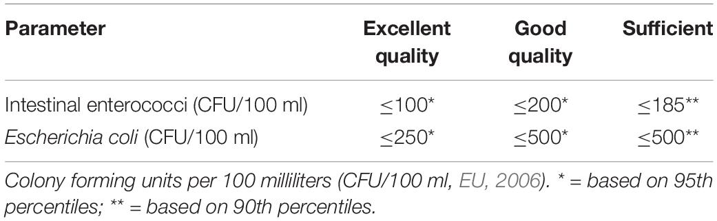
Table 1. Microbiological standards for coastal and estuarine (transitional) waters.

Surveys

Surveys of offshore oceanography at St Helena were carried out from the RRS James Clark Ross (survey JR17-004; 5th – 12th April 2018) and RRS Discovery (survey DY100; 5th – 14th April 2019). In 2019, inshore sites were sampled immediately after the offshore survey.

Study Sites

During both offshore surveys, field measurements were carried out at six stations around St Helena (Figure 1A). These stations were located on the 500 or 1000 m depth contour. In 2019, two new stations were located along a short transect outside James Bay extending from the station on the 500 m depth contour into shallower water (<50 m; Stations 14-16. Figure 1A).

FIGURE 1

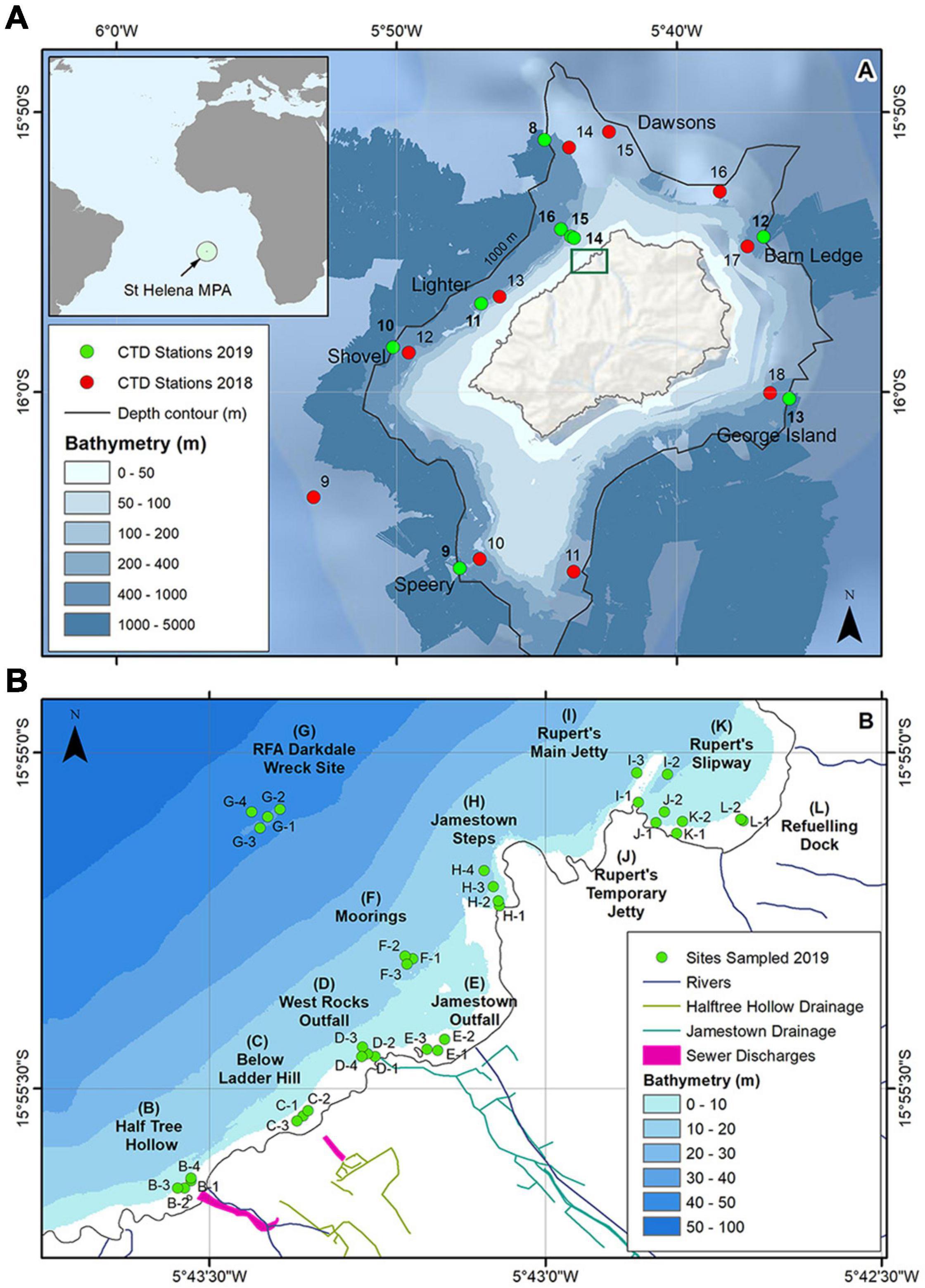
Figure 1. (A) Offshore CTD stations sampled at St Helena during the surveys; station numbers in 2019 are shown in bold; the inset shows the location of St Helena within the south Atlantic and the extent of the Marine Protected Area (MPA); the green rectangle shows where samples were collected inshore. (B) Inshore sampling locations; samples were obtained at one to four of the stations shown at each site. Nearshore bathymetry (≤500 m) reproduced by permission of the United Kingdom Hydrographic Office (UKHO) under delegated authority from The Keeper of Public Records (Crown Copyright). Basemap bathymetry from ESRI (2020).

In 2019, field measurements were made at eleven inshore sites (Figure 1B) using small boats, at one to four stations per site. Sites selected were those considered to be at greater risk from the impacts of human activities, such as sewage discharges and other land-based run-off (sites B, C, D, E, and H), fuel and other leakages (sites F and G), and fuel transfers (Rupert’s Bay jetties and refueling dock, sites I, J, K, and L, Figure 1B).

CTD Profiles and Sample Collection

Offshore

At each station, a CTD rosette was deployed to obtain profiles of water column structure. The sensor array included: a Seabird SBE11plus (temperature, °C; practical salinity; pressure, dbar), a Biospherical Licor Chelsea Sensor (downwelling Photosynthetically Active Radiation, μmol photons m^–2 sec^–1), a Chelsea Aquatracka MKIII fluorometer factory calibrated to an in-lab chlorophyll a standard (chlorophyll concentration, μg l^–1), a WET Labs ECO BB Scattering Meter (volume scattering coefficient, m^–1sr^–1, 2019 only), a SBE 43 Dissolved Oxygen Sensor (dissolved oxygen, μM).

In 2019, discrete sea water samples were collected for chlorophyll and nutrient analyses during the CTD upcast using 20-liter Niskin bottles mounted on the CTD rosette. The number of sampling depths ranged from one (just below the sea surface) to seven.

Inshore

At inshore sites (Figure 1B), a Valeport mini CTD was deployed to measure profiles of temperature and salinity. Discrete surface water samples were collected using clean 1-liter polypropylene buckets. Samples for nutrient and contaminant analysis were kept cool and transferred to the RRS Discovery for processing and/or storage.

Chlorophyll

Triplicate sea water sub-samples (250-1000 ml) from each depth sampled were filtered through 47 mm diameter glass microfiber filters (GF/F) using a Millipore filtration rig under low vacuum (<5 mm Hg). Filters were retained, folded, wrapped in aluminum foil and stored in a −80°C freezer.

Nutrients

On board the RRS Discovery, sea water (250-500 ml) from each depth sampled was filtered using a Millipore filtration rig with 47 mm diameter glass microfiber filter papers (GF/F) under low vacuum (<5 mm Hg). The initial filtrate was used to rinse the vacuum flask, and the remaining seawater was filtered into three 60 ml sample pots. Two were preserved with 0.1 ml of 16 g l^–1 mercuric chloride solution (final concentration approximately 28 mg l^–1) and stored in a refrigerator. The remaining sample was stored in a <-20°C freezer for ammonium analysis.

Chemical Contaminants

Pre-cleaned glass sample bottles (1 liter) were used to collect samples for contaminant screening. At each station, a bottle was uncapped, submerged by hand, filled with seawater from just below the surface, and re-capped. Nitrile gloves were worn throughout this process. All samples were stored in the dark during the sampling period and then transferred to refrigerators on the RRS Discovery for storage and transport back to the United Kingdom. The samples were transported in a refrigerated vehicle from the vessel to the analytical laboratory in the United Kingdom.

Fecal Indicator Bacteria

Surface seawater samples (250 ml) were collected directly into labeled, sterile plastic bags (500 ml). Samples were transferred within 1 h of collection to the microbiology laboratory at the St Helena Hospital where they were set up immediately to incubate as described below.

Surveys: Data and Sample Analysis

CTD Profiles

All offshore CTD profiles were extracted using SeaSave software (Version 7.26.7, Sea-Bird Scientific). Inshore profiles were extracted using Valeport Connect software (Version 1.0.7.10, Valeport Limited). All profiles were analyzed in Matlab 2019a (MathWorks, 2019). Down casts were isolated, and profiles binned by taking a mean over 0.5 m intervals for offshore profiles and 0.2 m intervals for inshore profiles. To smooth profiles a moving mean with a window size of 5 % of the data was applied.

Offshore profiles were analyzed individually and grouped by survey and location west or east of St Helena:

• East = RRS Discovery stations 12, 13; RRS James Clark Ross stations 11, 15, 16, 17, 18.

• West = RRS Discovery stations 8, 9, 10, 11, 16; RRS James Clark Ross stations 9, 10, 12, 13, 14.

Profiles were averaged by survey and region to show average depths (e.g., water column, upper mixed layer, thermocline, euphotic zone, fluorescence maximum, and low dissolved oxygen) and light attenuation co-efficients.

Temperature and salinity

Profiles of temperature, salinity, and pressure were used to calculate potential density following the methods of Gill (1982), using a reference pressure of 10 dbar. Mixed layer depth (MLD) was defined as the shallowest depth at which a density gradient of 0.005 kg m^–3dbar^–1 was reached, following the threshold method of Dong et al. (2008). Waters above this were considered to be the surface mixed layer (also referred to as the upper mixed layer, UML). The base of the seasonal thermocline was identified as the greatest depth at which a density gradient of 0.005 kg m^–3dbar^–1 was reached.

Temperature-salinity diagrams were created from offshore profiles of salinity, temperature, and pressure, with potential temperature calculated following Fofonoff and Millard (1983) using a reference pressure of 10 dbar.

Photosynthetically active radiation (PAR)

Where downwelling photosynthetically active radiation (PAR) data were available for profiles taken during daylight hours, downward attenuation coefficients of PAR (K_d(PAR)) were calculated following the Lambert-Beer equation:

$$E_d\left(z\right)=E_d\left(0\right).e^{-K_{d}z}$$

where E_d(z) is downward irradiance available at a certain depth (z), E_d(0) is the downward irradiance available just below the surface, and K_d is the vertical attenuation coefficient for downwards irradiance between the surface and depth z (Kirk, 1994).

A linear regression of ln-transformed E_d vs. depth between the depth of the shallowest PAR value (often 0.5 m) and the depth at which E_d reached 1 μmol photon m^–2 s^–1 was used to derive K_d(PAR).

The depth of the euphotic zone (Zd) was approximated by 4.6/K_d, as per Kirk (1994), as K_d was observed to be relatively constant with depth.

Fluorescence

Sensor fluorescence values were validated using discrete chlorophyll measurements to confirm that factory calibrated fluorescence-to-chlorophyll ratios were appropriate for St Helena waters.

Turbidity

Turbidity values were occasionally below zero, presumably due to calibration error. To correct for this, negative turbidity values were set to zero.

Dissolved oxygen

Theoretical oxygen saturation profiles were calculated as a function of temperature and salinity assuming equilibrium with the atmosphere, as described in Garcia and Gordon (1992).

Chlorophyll Concentrations

Samples were returned to the United Kingdom and stored in a −80°C freezer for analysis by High Performance Liquid Chromatography (HPLC) as described in Hooker et al. (2005) in October 2019. The glass microfiber filters were transferred to vials with 6 ml 95% acetone and internal standard (vitamin E). Samples were mixed on a vortex mixer, sonicated on ice, extracted at 4°C for 20 h, and mixed again. Samples were then filtered through 0.2 μm Teflon syringe filters into HPLC vials and placed together with mixed pigments standards (DHI, Denmark) in the cooling rack of the HPLC system (Shimadzu LC-10A HPLC system with LC Solution Software). Buffer and samples were injected onto the HPLC system in the ratio 5:2 using a pre-treatment program and mixing in the loop before injection.

Total chlorophyll a concentrations (μg l^–1) were the sum of chlorophyll a from Prochlorococcus spp. and from all other algae. The limit of detection was 0.02 μg l^–1 for 250 ml filtered samples and 0.005 μg l^–1 for 1000 ml filtered samples. The uncertainty of the method is <1.0%.

Measured chlorophyll concentrations were used to validate sensor fluorescence values (see above). Average values were calculated for the upper mixed layer, the seasonal thermocline, and deeper bottom waters (generally > 150 m).

Nutrients

Samples were returned to the United Kingdom and stored in a refrigerator or freezer prior to analysis. A subset of the frozen sub-samples was defrosted and analyzed for nutrients in August/September 2019.

Analyses were performed on a Skalar San++ Continuous Flow Analyser (CFA) (Skalar Analytical B.V, Breda, Netherlands) running channels for nitrite, phosphate, silicate and ammonium with photometric detection, as described in Bendschneider and Robinson (1952), Murphy and Riley (1962), Treguer and LeCorre (1975), Grasshoff (1976).

Samples were analyzed for nitrite-N, TOxN (nitrite+nitrate), ammonium-N, phosphate-P and silicate-Si. Total dissolved inorganic nitrogen (DIN) was calculated by summing TOxN and ammonium. Limits of detection were 0.07 μM for nitrite, 0.43 μM for ammonium, 0.14 μM for phosphate, and 0.09 μM for silicate.

For offshore samples, average values were calculated for surface waters (the upper mixed layer), the seasonal thermocline, and deeper bottom waters (>150 m). Average values of DIN and phosphate-P were used to calculate N:P ratios for comparison against Redfield ratios for N:P (16:1) and N:Si (∼1:1) (Downing, 1997; Lefevre et al., 2003; Burson et al., 2016). Values below the limits of detection were set to 0.01 μM and were not used to calculate nutrient ratios.

Chemical Contaminants

Samples were screened using a gas chromatography-mass spectrometry (GC-MS) technique for non-polar organic environmental pollutants (Smith et al., 2015; Gravell et al., 2013; Sandy and Civil, 2014; White et al., 2019; Sorensen et al., 2015).

The technique allows for a target based, multi-residue screening of volatile organic compounds (VOCs) and semi-volatile organic compounds (SVOCs). The method uses a retention time locked, custom built target mass spectrometric database with over 1050 compounds, allowing for the identification and measurement of a wide range of organic pollutants in any given water body. It applies deconvolution reporting software to provide increased confidence in identifying the chemical peaks in each sample. For each contaminant detected in the screening process, a chemical database was used to describe the possible sources and/or use of the chemicals.

Screening results are semi-quantitative and useful for indicating the presence of chemicals at concentrations in the μg l^–1 range that may need further investigation and quantification. Estimated concentrations are indicative only and it is not generally considered appropriate to use these to determine if chemicals detected are at acceptable or unacceptable concentrations. Nonetheless, international standards were used to identify potential risks from chemical contaminants, particularly substances of very high concern (SVHC, EC, 2006; EU, 2006) and priority substances (EU, 2008b, 2013, 2016).

Fecal Indicator Bacteria

Samples were analyzed at the St Helena Public Health Laboratory at the General Hospital in Jamestown. The number of colony forming units of total coliforms and E. coli were enumerated using standard methods (SCA, 2016) following ISO guidelines (ISO, 2018). For each sample, up to 100 ml of water was filtered onto two 47 mm, 0.45 μm pore-size cellulose nitrate filter membranes. The filters were placed onto an absorbent pad that was saturated with membrane lauryl sulfate broth (MLSB) in a Petri dish. Petri dishes were incubated at 30°C for a 4-h recovery step. Following recovery, one Petri dish was incubated at 37°C and the other at 44°C for at least 14 h for each sample. After incubation, yellow colonies on the membranes incubated at 37°C were counted as presumptive coliforms and yellow colonies on the membranes incubated at 44°C were counted as presumptive E. coli.

Results

Model and Satellite Data

Oceanographic Background Conditions

Temperature and salinity

Strong seasonal patterns were observed in the model temperature data (Figure 2A), with lower surface temperatures in late winter to early spring (minimum ca 20°C in September), increasing to higher values in late summer to early autumn (maximum ca 26°C in March). The depth of the upper mixed layer varied each year; average conditions showed a thermocline at approximately 100 m which was deeper in late winter to early spring.

FIGURE 2

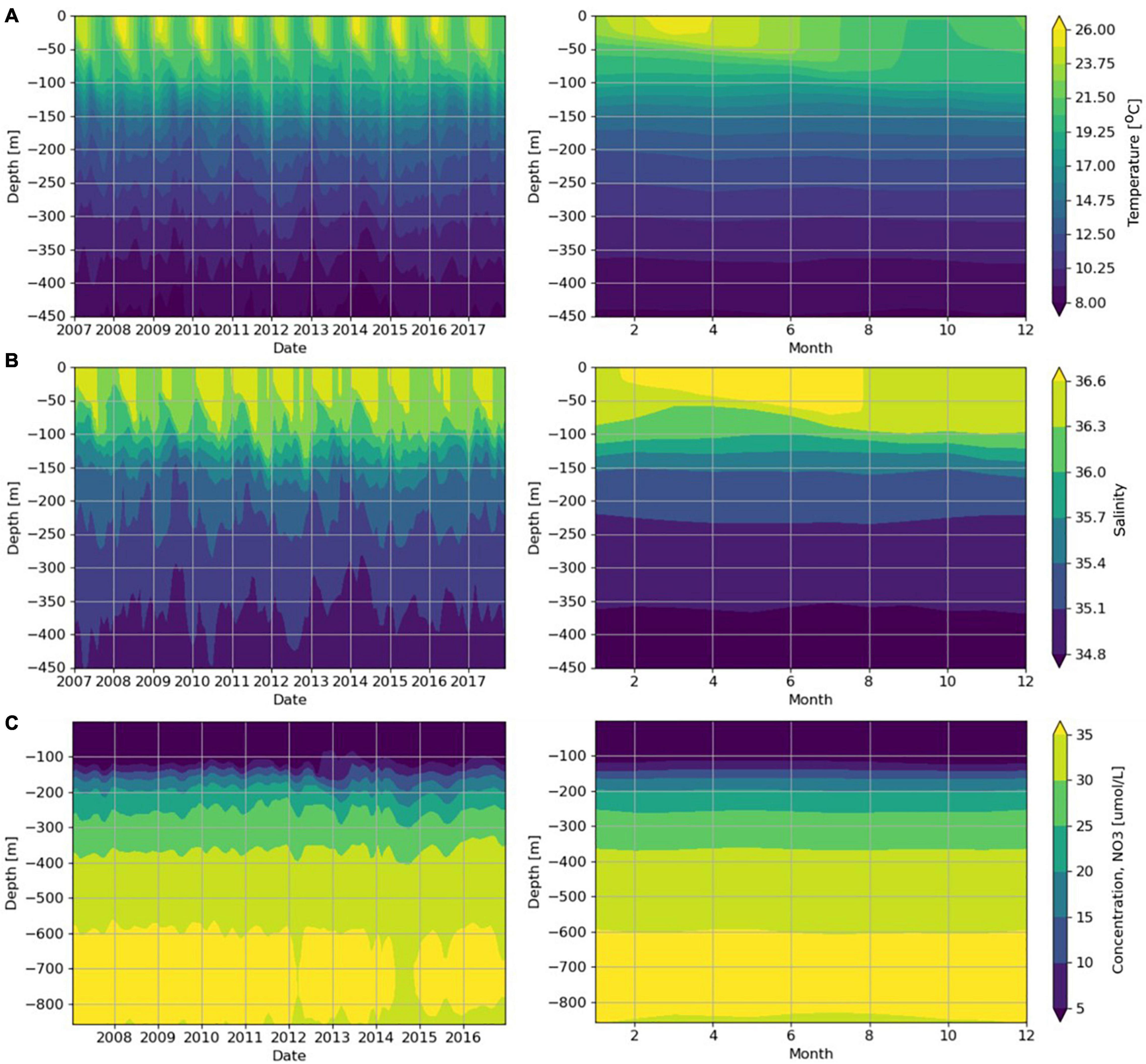
Figure 2. Temperature, salinity and nitrate (NO₃) profiles, from model analysis (2007-2017) at 16°S, 5.75°W. (A) temperature (°C), (B) salinity, (C) nitrate (μM); note change of scale on y-axis. Left = time-series of monthly averages; right = monthly climatology.

Model surface salinities also showed a seasonal cycle (Figure 2B), with lower values during spring in the upper mixed layer (minimum of ca 36.4 in November). Throughout the year, salinity values were typically higher in the upper mixed layer and decreased with depth. Salinity data also indicated that the average depth of the upper mixed layer was around 100 m.

Nutrients, chlorophyll, and SPM

Seasonal trends were observed in model and satellite concentrations of surface nutrients, chlorophyll and SPM (Figures 3A-C). Maximum values were 1.86 μM for nitrate, 0.78 μg l^–1 for chlorophyll and 1.6 mg l^–1 for SPM (Figures 3A-C). Below the thermocline, nitrate concentrations were high, increasing to >30 μM below approximately 350 m depth (Figure 2C).

In surface waters, average monthly nitrate concentrations were low (close to or at zero) from January to May and increased from June to November, with maximum values in September (spring, Figure 3D). From these monthly climatologies, average background values for nitrate from June to November (seasonal average, Table 2a) were calculated to be 0.12 μM. Similarly, average background values were estimated to be 0.17 μM for phosphate and 1.57 μM for silicate (Table 2a). Using data from all months, the annual average for nitrate (0.06 μM, Table 2a) was lower than the seasonal average. For phosphate and silicate, annual averages were similar to seasonal averages. N:P and N:Si ratios from seasonal averages (0.7:1 and 0.1:1, respectively, from seasonal averages in Table 2a) were lower than Redfield ratios. At depth (150-500 m), annual averages were high (26.78 μM for nitrate, 1.81 μM for phosphate and 17.27 μM for silicate, Table 2a); N:P and N:Si ratios (15:1 and 1.6:1, respectively) calculated from annual averages were close to Redfield ratios.

TABLE 2

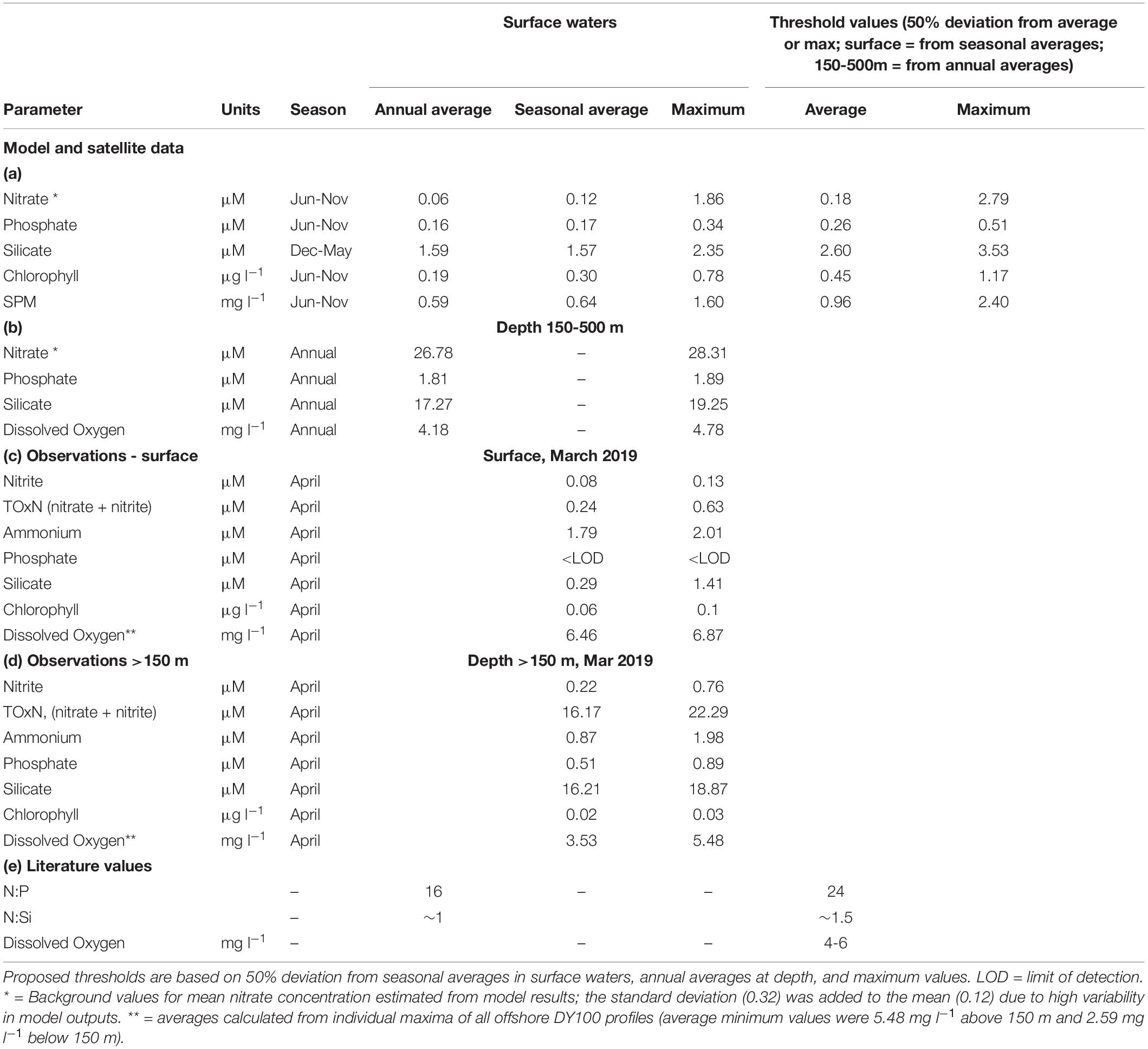
Table 2. Background values for (a) surface waters from model output (2007-2016) and satellite products (1998-2017), shown as annual averages, seasonal averages (months with highest natural values, e.g. June to November, Figure 3) and maximum values; (b) 150-500 m from model outputs, shown as annual averages and maximum values. Averages from offshore survey data (see Table 4) are shown for (c) surface water (the upper mixed layer) and (d) deep water (>150 m). (e) Threshold values taken from the literature.

Chlorophyll and SPM concentrations (available as surface values only) showed inter-annual variability in precise timings and peak values (Figures 3B,C). Average monthly concentrations showed similar trends to nitrate concentrations; they were low (ca. 0.1 μg chl l^–1, Figure 3E; 0.5 mg l^–1 for SPM, Figure 3F) from January to May, increasing to reach a peak in October (0.38 μg chl l^–1) or September (0.7 mg l^–1 for SPM). Seasonal averages (Table 2) were calculated to be 0.3 μg chl l^–1 and 0.64 mg l^–1 for SPM. Annual averages for chlorophyll (0.06 μg chl l^–1, Table 2) and SPM (0.59 mg l^–1) were lower than seasonal averages.

FIGURE 3

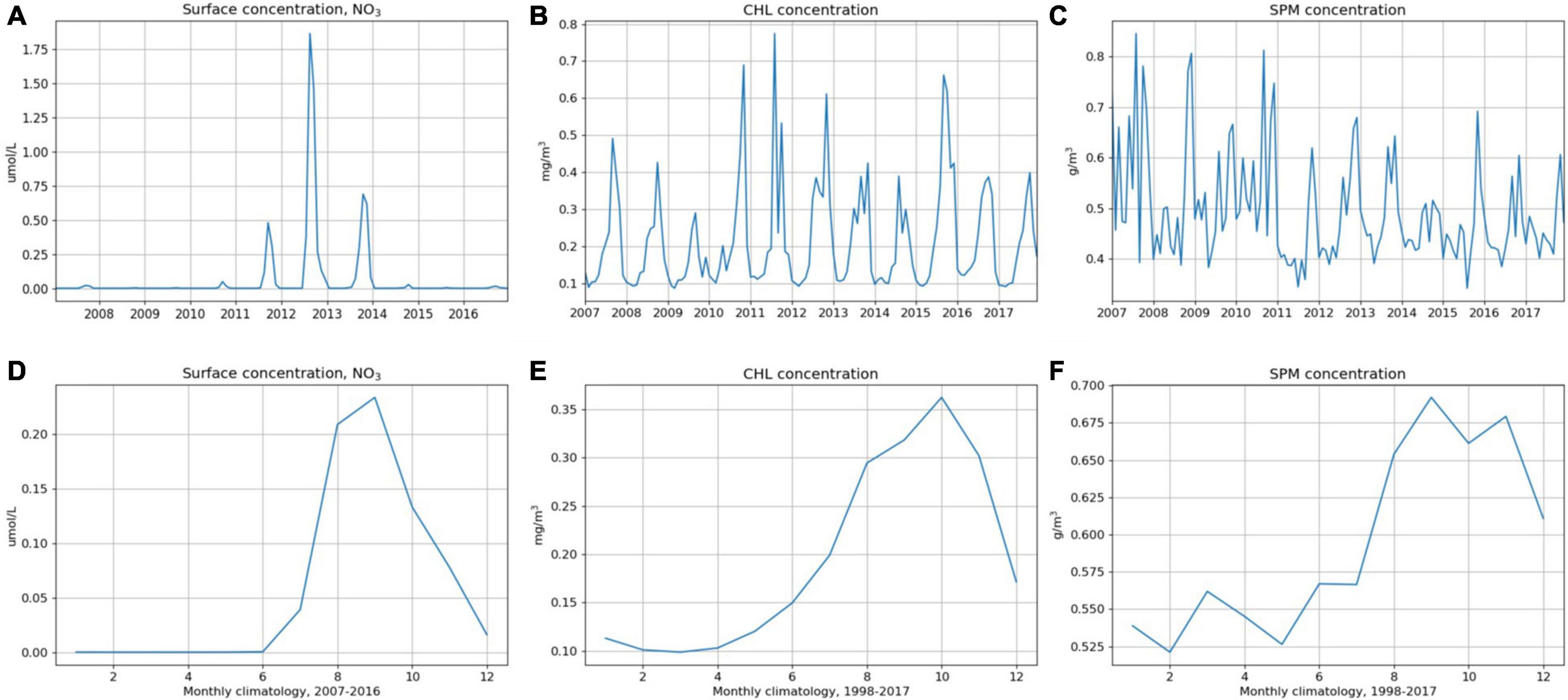
Figure 3. Time-series of monthly averages in surface waters shown in top panel (A) nitrate (NO₃) concentration (μM) at 16°S, 5.75°W (see Figure 2); (B) chlorophyll (Chl) concentrations (mg m^–3) and (C) SPM concentrations (g m^–3) in a 25 km × 25 km grid around St Helena Island, from satellite data. Monthly climatology in surface concentrations shown in bottom panel (D) NO₃ (2007-2016), (E) Chl (1998–2017), and (F) SPM (1998-2017).

Proposed Thresholds

Thresholds based on seasonal averages and maximum values in surface waters (Table 2) were proposed for nitrate (average = 0.18 μM, max = 2.79 μM), phosphate (average = 0.26 μM, max = 0.51 μM), silicate (average = 2.60 μM, max = 3.53 μM), chlorophyll (average = 0.45 μg chl l^–1, max = 1.17 μg chl l^–1), and SPM (average = 0.96 mg l^–1, max = 2.40 mg l^–1).

Survey Observations

CTD Profiles

Offshore waters

All offshore profiles of temperature and salinity (Figures 4, 5 and Supplementary Figure 1–6) displayed an upper mixed layer (UML) of uniform physical structure within the upper 10-30 m of the water column. Between the UML and 150-230 m depth, a seasonal thermocline of rapidly changing temperature was observed. Below this a deeper permanent thermocline was present where temperature and salinity changed slowly with depth until approximately 1 km depth where intermediate water masses were found.

FIGURE 4

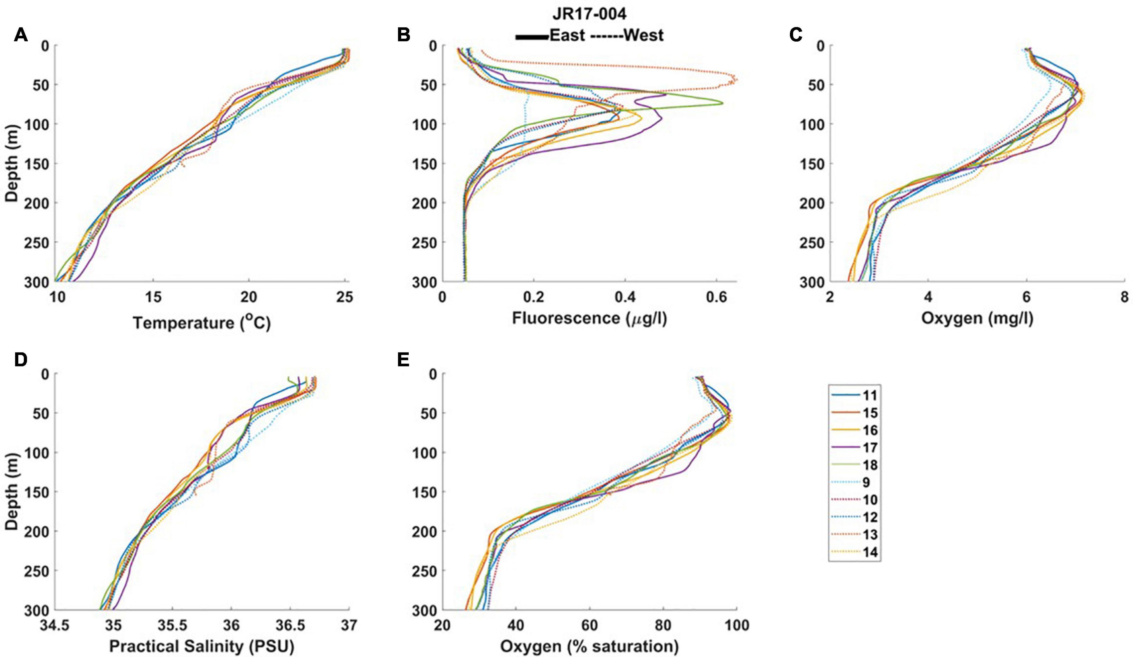
Figure 4. Profiles from RRS James Clark Ross (2018) of (A) temperature, (B) fluorometric chlorophyll, (C) oxygen concentration, (D) practical salinity, and (E) oxygen saturation, from east and west stations. The legend shows the CTD profile numbers.

FIGURE 5

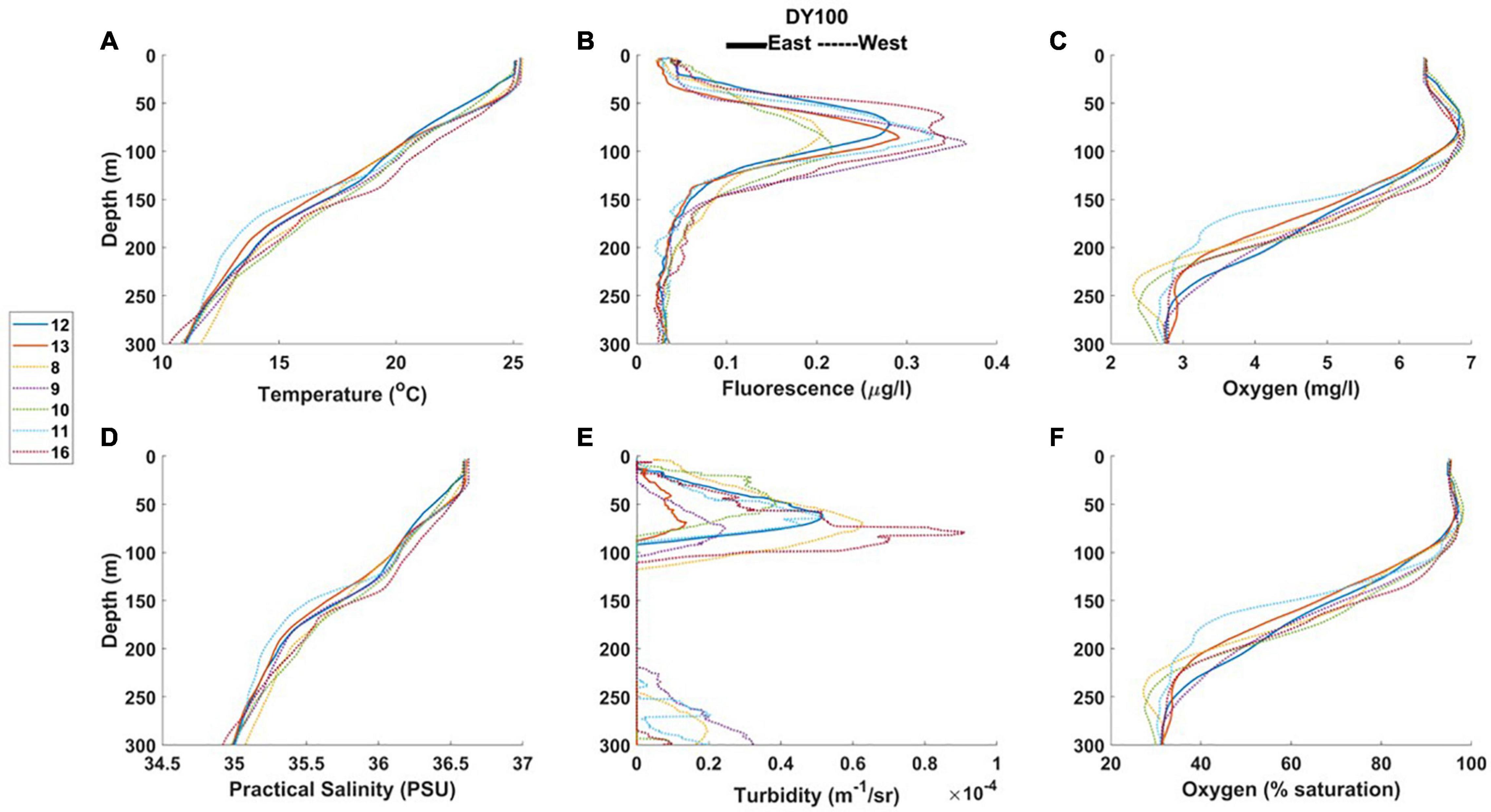
Figure 5. Profiles from RRS Discovery (2019) of (A) temperature, (B) fluorometric chlorophyll, (C) oxygen concentration, (D) practical salinity, (E) turbidity, and (F) oxygen saturation, from east and west stations. The legend shows the CTD profile numbers.

At the seasonal thermocline, a deep fluorescence (chlorophyll) maximum was observed in all profiles (Figures 4, 5; average values 0.29 to 0.46 μg chl l^–1, Table 3). The chlorophyll maximum was accompanied by a turbidity maximum (Figure 5), an oxygen maximum (>6 mg l^–1, Figures 4, 5), and oxygen saturation levels close to 100% (Figures 4, 5). All profiles displayed oxygen deficiency (<4 mg l^–1) in waters below the seasonal thermocline (Table 3), averaging 3.53 mg l^–1 at all depths > 150 m (Table 2).

TABLE 3

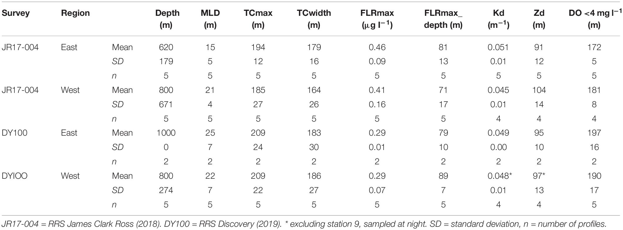
Table 3. Summary of offshore CTD profiles averaged by survey and region (east and west of St Helena) showing water column depth (depth), mixed layer depth (MLD), maximum (max) depth and width of the seasonal thermocline (TC), the fluorescence maximum (FLRmax, μg chlorophyll l^–1 and depth), the light attenuation co-efficient (Kd), the maximum depth of the euphotic zone (Zd), and the depth below which dissolved oxygen (DO) was <4 mg l^–1.

In 2018 (JR17-004) the MLD of the upper mixed layer was on average 6 m deeper on the west side of the island, with a narrower region of rapidly changing density in the seasonal thermocline than on the east side (Table 3). The average maximum fluorescence value was 0.07 μg l^–1 higher in easterly stations. On average, fluorescence maxima were higher on the easterly side of the island. The highest fluorescence value was, however, observed at Station 13 in the west (see Figure 1).

In 2019 (DY100) the MLD was similar on the eastern and western side of the island, as was the width of the seasonal thermocline (Table 3). Average maximum fluorescence values were similar in both regions, although the depth of the fluorescence maximum was on average 10 m deeper in the west. Optical properties of the water column were, on average, very similar. Profiles indicate that the observed oxygen maximum generally extended deeper at westerly stations, and minimum oxygen values were typically lower in the west (Figures 5C, F). Although, on average, fluorescence maximum values were similar between easterly and westerly stations (Table 3), highest fluorescence values were observed in the west (Figure 5B), as were highest turbidity maxima (Figure 5E). A deep turbidity maximum was also observed in the west (Figure 5E).

Temperature-salinity plots

Temperature-salinity (T-S) plots of offshore profiles from both surveys (Figure 6) allowed comparison of the water column against the typical characteristics of water masses in the region (Tomczak, 1999). The temperature and salinity characteristics of deep waters offshore of St Helena fall within ranges typical of South Atlantic Central Water at approximately 6°C–16°C and salinity 34.5-35.5 (linear section in Figure 6), Antarctic Intermediate Water, characterized by a salinity minimum at depth, with a core temperature of 4–5°C and salinity minima between 34.2 and 34.5, and North Atlantic Deep Water with a salinity greater than 34.8 (Steele, 2001). Figure 6 shows some level of variability in the warmer (>12°C) surface waters around St Helena, with T-S lines for the two surveys displaying slightly different behavior.

FIGURE 6

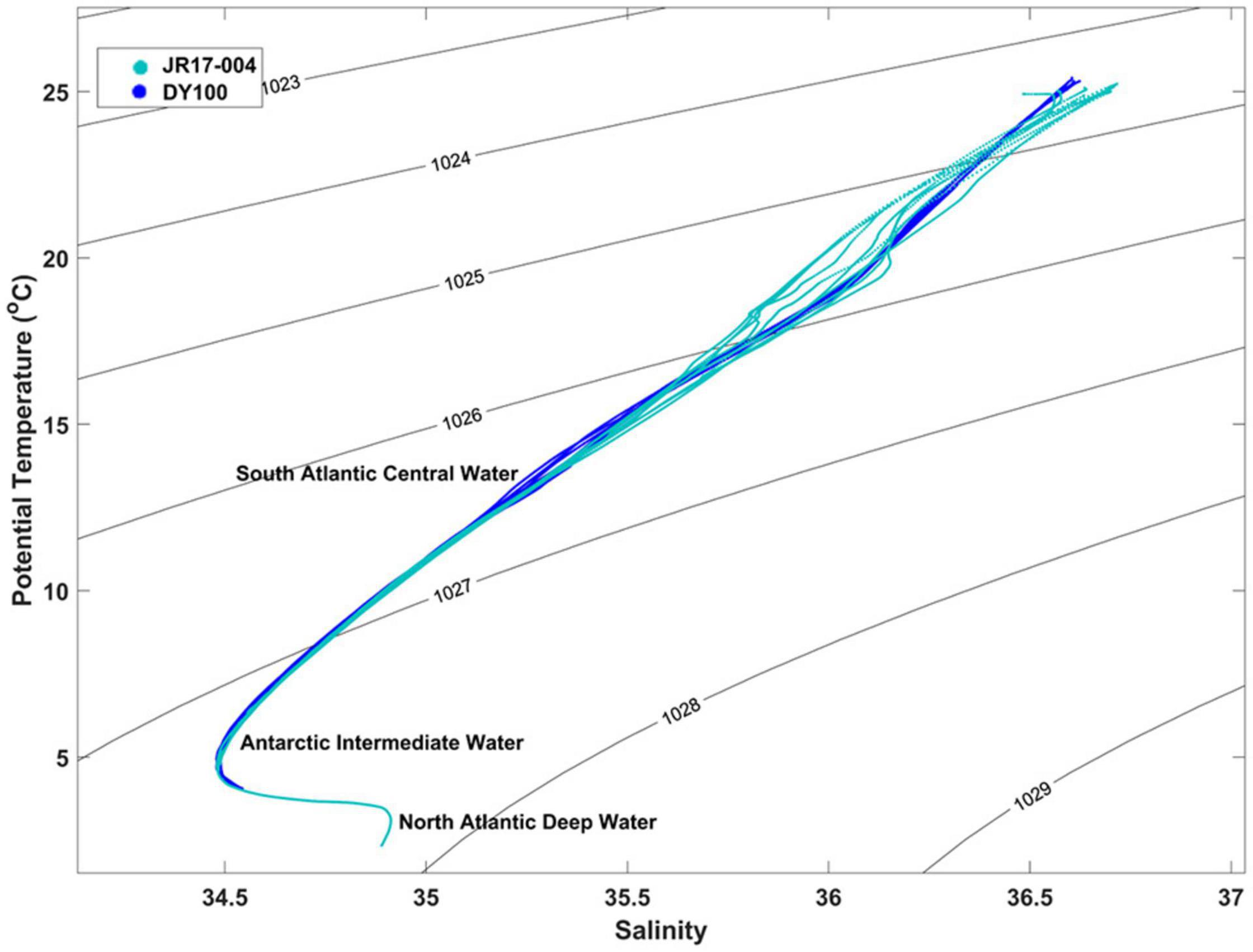
Figure 6. T-S plot of selected CTD profiles from RRS James Clark Ross and RRS Discovery, including contours of uniform density showing typical signatures of South Atlantic Central Water, Antarctic Intermediate Water, and North Atlantic Deep Water.

James Bay transect

At the deepest station (Station 16, 500 m), profiles were similar to other offshore stations, with a chlorophyll maximum (0.3 μg l^–1) at approx. 90 m (Figure 7, Table 3, and Supplementary Figures 3, 7). At the intermediate station (Station 15 ± 120 m water depth), the upper 30 m was well mixed with low chlorophyll concentrations (<0.1 μg chl l^–1) and high levels of dissolved oxygen (>6 mg l^–1, Supplementary Figure 3). Below 30 m, there was a gradual decrease in temperature and salinity; chlorophyll concentrations increased to a maximum of 0.4 μg l^–1 at 40 m, where turbidity levels were also higher (approx. 1 m^–1/sr; Supplementary Figure 3). At the shallow (50 m) innermost station (Station 14, see Figure 1), the water column was vertically mixed, with low chlorophyll concentrations (<0.1 μg chl l^–1) and high levels of dissolved oxygen (>6 mg l^–1, Supplementary Figure 3).

FIGURE 7

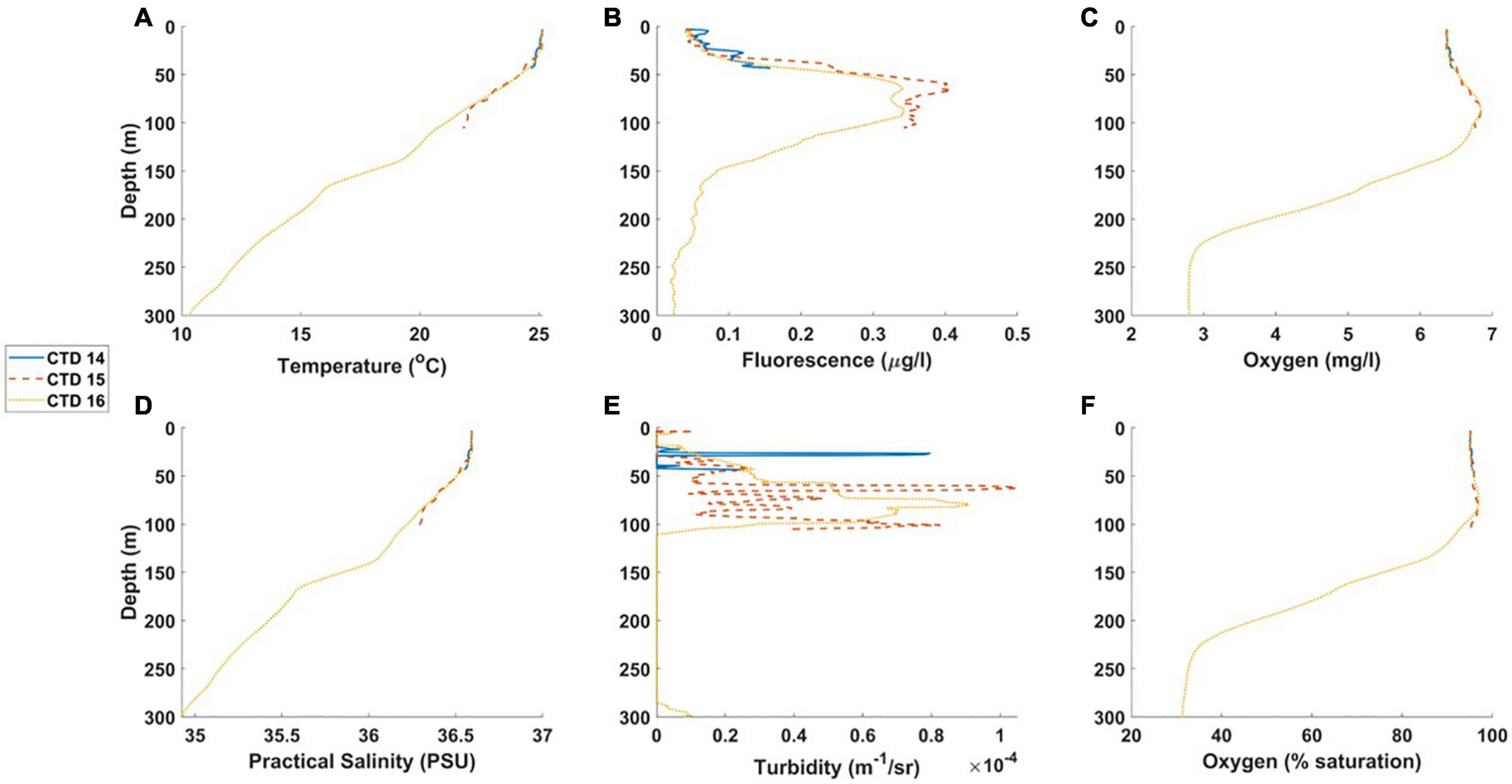
Figure 7. (A-F) CTD profiles from the James Bay transect, DY100: Station 16 = furthest offshore; Station 14 = closest to James Bay. The legend shows the CTD profile numbers.

Inshore sites

Temperature and salinity profiles (Supplementary Figure 8) showed that the water column was generally mixed at all inshore sites. Water temperatures ranged from 24.5 to 25.1°C and salinities from 36.62 to 36.75. Average values (24.8°C, salinity 36.70) were similar to averages in the UML at all offshore stations (Figure 5) around St Helena (25.2°C, salinity 36.60) and along the James Bay transect (25.1°C, salinity 36.59).

Chlorophyll

Chlorophyll measurements confirmed that factory calibrations of sensor fluorescence were valid for St Helena. At depth, the relationship between the factory calibration and discrete samples was approximately 1:1, with some instances in shallower water where discrete samples returned slightly higher chlorophyll concentrations.

Discrete samples showed that average chlorophyll concentrations (Table 2) were low in surface waters (0.06 μg l^–1, average depth 7 m), higher in samples taken at around 100 m (0.5 μg l^–1, not shown) and low (0.02 μg l^–1, Table 2) below the thermocline, at an average sample depth of 458 m.

Nutrients

Offshore waters

In offshore surface waters, nutrient concentrations were generally low (<1 μM, Table 4), except for ammonium (average = 1.79 μM) and therefore DIN (average = 2.04 μM). Dissolved inorganic phosphate concentrations were below the detection limit. At the two outermost stations (Stations 15 and 16) on the James Bay transect, concentrations of silicate were relatively high in the UML and thermocline region compared with most other stations (Table 4).

TABLE 4

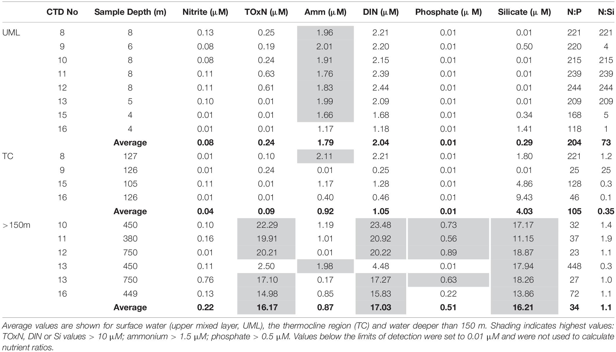
Table 4. Offshore concentrations of dissolved inorganic nutrients (μM) during the 2019 survey (DY100).

In deep (>150 m) offshore water, concentrations of TOxN, DIN, and silicate were high (>10 μM) at all stations (Table 4). Nitrate was the main contributor to DIN concentrations.

In surface waters, the average nutrient ratio (using DIN for nitrogen) was not calculated for N:P (Table 4), due to phosphate concentrations consistently below the limit of detection (LOD). The average ratio for N:Si (3:1, Table 4) was three times higher than the Redfield ratio of ∼1:1. In the thermocline region, the N:P ratio was not calculated due to low phosphate values (<LOD) and the average N:Si ratio (0.5:1) was lower than in surface waters and approximately half the Redfield ratio. In deep water (>150 m), the average N:P ratio was 34:1 (Table 4), approximately two times higher than the Redfield ratio. The N:Si ratio (1.1:1, Table 4) was close to the Redfield ratio.

Inshore sites

Nitrite and TOxN values were generally low at all inshore sites (Table 5). Average and maximum values were (respectively): 0.16 μM and 0.44 μM for nitrite, and 0.23 μM and 1.47 μM for TOxN. However, most nitrite values were higher than the average value in offshore surface water (0.08 μM, Table 4) and TOxN was higher than the surface offshore average (0.24 μM, Table 4) at two sites in James Bay (West Rocks outfall, D2, and Jamestown Steps, H1) and two sites in Rupert’s Bay (Rupert’s Slipway, K1, and the Refueling Dock, L1; Table 5).

TABLE 5

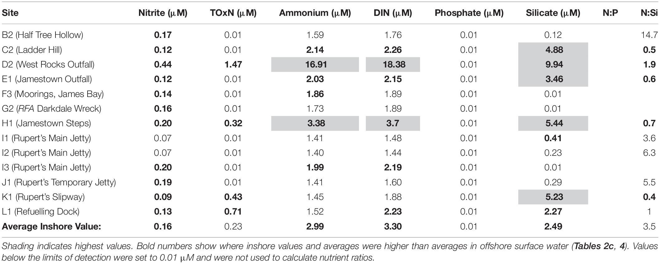
Table 5. Concentrations of dissolved inorganic nutrients (μM) at all inshore sites sampled (surface water) in 2019.

Concentrations of ammonium were relatively high at all inshore sites (Table 5), with average and maximum values of 2.99 and 16.91 μM. Due to high ammonium concentrations, inshore values for DIN were also high (average 3.3 μM, maximum 18.38 μM, Table 5). Highest ammonium and DIN values were estimated at West Rocks Outfall (site D2) and Jamestown Steps (site H1, see Figure 1B).

Dissolved inorganic phosphate concentrations were below the detection limit at all sites (Table 5). Ratios of N:P were therefore not calculated.

Silicate concentrations were variable, with average and maximum values of 2.48 μM and 9.94 μM, respectively (Table 5). The average N:Si ratio was 3.5:1, approximately three times higher than the Redfield ratio of ∼1:1.

Average inshore nutrient concentrations (Table 5) were generally higher than average nutrient concentrations in offshore surface water (Tables 2b, 4) (inshore: 0.16 μM nitrite, 2.99 μM ammonium, 3.30 μM DIN, 2.48 μM silicate; offshore: 0.08 μM nitrite, 1.79 μM ammonium, 2.04 μM DIN, 0.29 μM silicate). Average concentrations of TOxN were comparable (0.23 μM inshore and 0.24 μM offshore).

Average inshore concentrations for most nutrient were lower (Table 5) than average nutrient concentrations in deep (>150 m) offshore water (Table 2c) (inshore: 0.16 μM nitrite, 0.23 μM TOxN, 3.3 μM DIN, 2.48 μM silicate; offshore: 0.21 μM nitrite, 16.71 μM TOxN, 17.03 μM DIN, 0.51 μM phosphate, 16.21 μM silicate). Ammonium concentrations were higher (2.99 μM inshore, 0.87 μM offshore).

Chemical Contaminants

Contaminants listed as Priority Substances under the European Water Framework Directive, (2000/60/EC) and substances of very high concern (EU, 2006) that are amenable to the GC-MS screen were absent from the results.

Low levels of contaminants of concern were detected in the samples analyzed, including bromoform, 2,4,6-tribromophenol, dibromomethane, and N, N-Diethyl-meta-toluamide (DEET).

The greatest number of contaminants (eight, Figure 8A) was detected at West Rocks outfall (Site D, Figure 1B). At all other sites, five or fewer chemical contaminants were detected (Figure 8A). In total, 14 different contaminants were detected in the inshore samples (Figure 8B; see Supplementary Table 1).

FIGURE 8

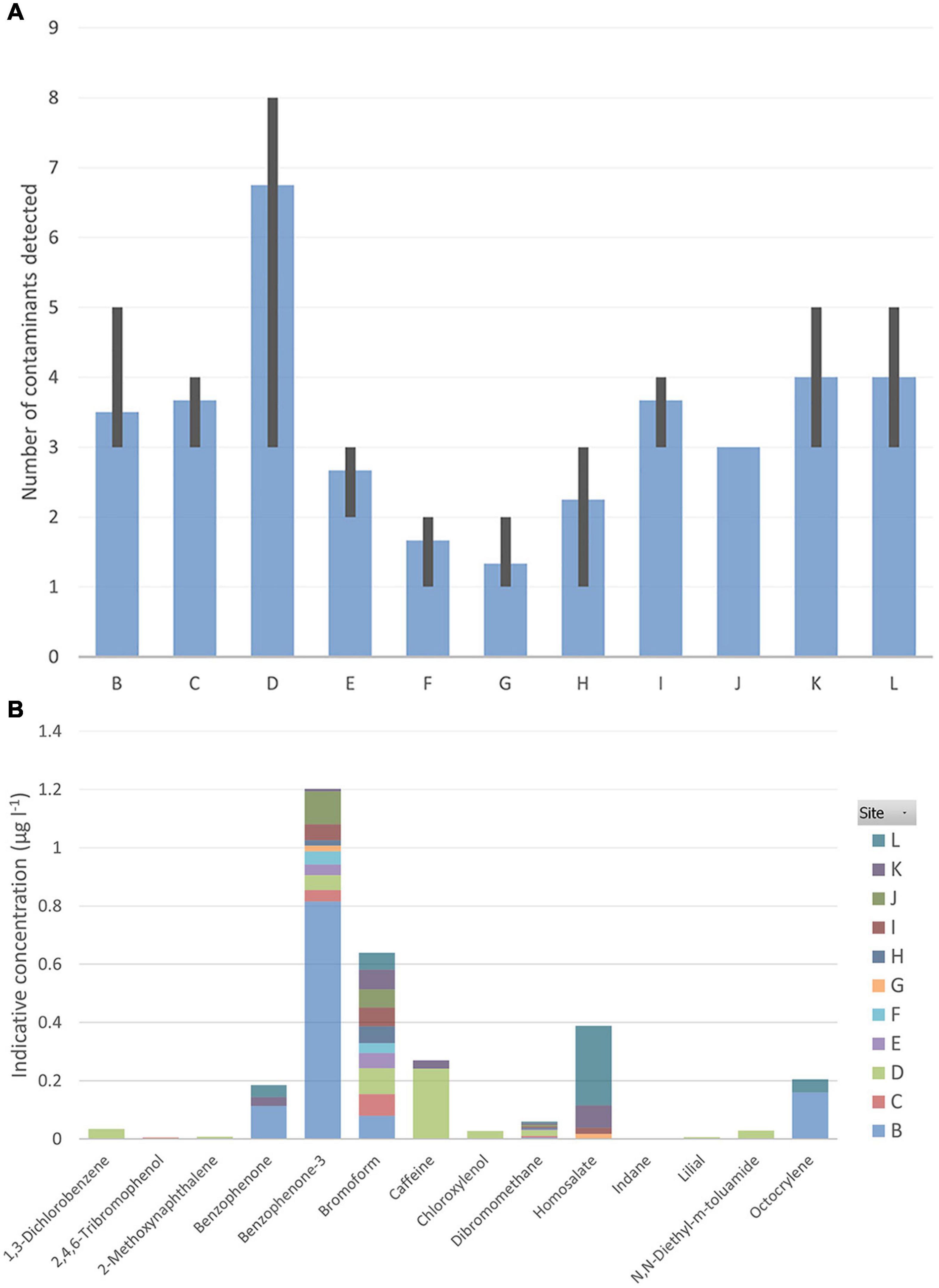
Figure 8. (A) Average number of contaminants detected at each inshore site (B-L) with minimum and maximum values per station shown as error bars; (B) Average indicative concentration (in μg l^–1) of contaminants detected at each inshore site.

Benzophenone-3 (a personal-care product), bromoform and dibromomethane (volatile solvents used for a range of purposes from agrochemical intermediates to refrigerant precursors to degreasing solvents) were the most frequently occurring chemicals, found at 25-30 stations (e.g., Jamestown Outfall (site E), Jamestown steps (site H), Rupert’s Bay temporary jetty (site J) [Supplementary Table 1]). Benzophenone-3 and bromoform were also identified at James Bay Moorings (site F).

At Rupert’s Bay main jetty (site I), bromoform was recorded at a relatively high concentration (>0.1 μg l^–1, Supplementary Table 1), as well as homosalate (sunscreen UV filter) at low concentrations. At Rupert’s Bay temporary jetty, benzophenone-3 was recorded at a relatively high concentration (>0.1 μg l^–1). At Half Tree Hollow (site B), benzophenone, benzophenone-3 and octocrylene (a UV-filter) were found at relatively high concentrations (∼0.11, ∼3.1, and ∼0.16 μg l^–1, respectively).

At Ladder Hill (site C), the most commonly occurring chemicals identified were the volatile solvents, benzophenone-3, bromoform and dibromomethane (all at low concentrations of <0.1 μg l^–1, Supplementary Table 1). A pesticide, 2,4,6-tribromophenol, was also detected here, at low concentrations (<0.005 μg l^–1).

At West Rocks Outfall (site D), the most commonly occurring chemicals were volatile solvents (all at low concentrations of <0.1 μg l^–1, Supplementary Table 1). Caffeine and bromoform were recorded at relatively high concentrations (each >0.1 μg l^–1).

Benzophenone-3 and homosalate (sunscreen UV filter) were detected in one sample from the wreck of RFA Darkdale (G4).

Fecal Indicator Bacteria

Total coliform and E. coli concentrations ranged from <20 CFU/100 ml (at several locations) to >300 CFU/100 ml at West Rocks Outfall (Table 6) for both total coliforms and E. coli. Untreated sewage is discharged here, and it is adjacent to one of the main swimming areas on the Island. At other inshore sites sampled, counts were <100 CFU/100 ml (Table 6).

TABLE 6

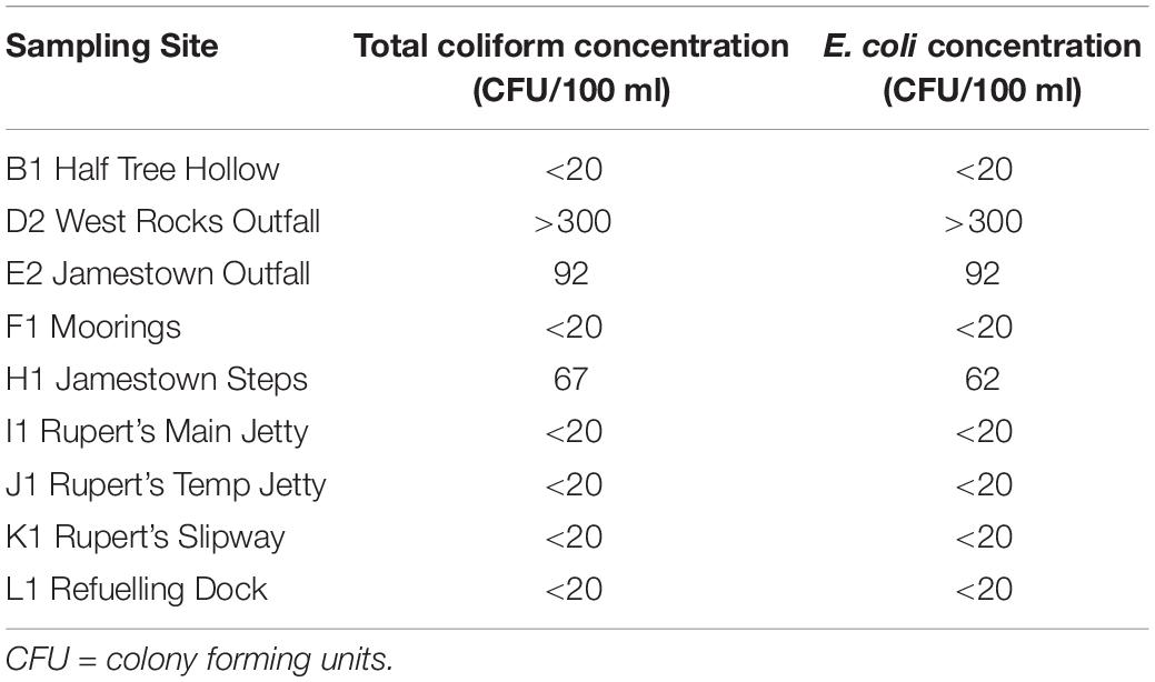
Table 6. Total colony counts of coliforms and Escherichia coli at nine of the sites sampled in 2019.

Discussion

Oceanographic Background Conditions

In the absence of long-term data at St Helena, model and satellite outputs provided valuable data for estimating the oceanographic background conditions at St Helena, particularly over large temporal and spatial scales. To identify annual and seasonal trends in chlorophyll and SPM relevant to St Helena, ocean color data were restricted to a relatively small area around (ca 25 km × 25 km) around the island. As for all remotely sensed data, outputs were for surface waters only. Model outputs provided comparable information on trends in concentrations of dissolved inorganic nutrients and dissolved oxygen. Moreover, they provided outputs based on vertical distributions through the water column. These outputs showed that nutrient concentrations were low (<2 μM nitrate and <0.5 μM phosphate) in surface waters and high (up to 40 μM nitrate and 1.5 μM phosphate) in waters below the thermocline present at around 100 m. In surface waters, monthly climatologies in both model and satellite outputs indicated seasonal trends, with June to November likely to represent the period of highest productivity. During these months, the water column was less stratified, possibly allowing nutrient-rich water to mix with shallower waters in the thermocline region.

Offshore observations were consistent with model results, even though the surveys (both in April) were earlier than the season with highest surface productivity. Field measurements clearly showed the presence of a sub-surface chlorophyll maximum in the thermocline region. These chlorophyll maxima are a frequent occurrence in many marine ecosystems (e.g., Herbland et al., 1985; Bauerfeind, 1987; Wasmund et al., 2005; Lett et al., 2007; Lund-Hansen, 2011; Cullen, 2015; Baldry et al., 2020) and are thought to occur due to the interplay of many factors including light, nutrient availability and grazing. Discrete samples showing that chlorophyll values in surface waters may be higher than data from remote sensing suggest that surface sensed chlorophyll data should be taken as indicative. Furthermore, discrete measurements showing surface chlorophyll values slightly higher than fluorometrically sensed values may indicate that non-photochemical quenching of fluorescence values may occur in the high light environment in surface waters. Correction of the fluorescence to chlorophyll relationship requires greater understanding of surface mixing and physiology of species in surface waters (Xing et al., 2018).

N:P ratios lower than the Redfield ratio (e.g., in the model) potentially indicate that not all nitrogen sources (such as ammonium) are taken into consideration or that seasonal or annual averages are not able to reflect short-term changes in nutrient and phytoplankton dynamics. Phosphorus concentrations below the limit of detection of the analytical instrument may indicate phosphorus limitation of phytoplankton communities in surface and thermocline waters. Relatively high observed N:P values (34:1) in waters deeper than 150 m were within the ranges reported in the literature (e.g., Downing, 1997) but may suggest limited phosphorus concentrations in source waters. Model and observed nitrogen to silicate ratios in line with Redfield ratios of ca 1:1 in deeper water (>150 m) suggest that silicate concentrations here were in balance with nitrogen in source waters. Low N:Si ratios (in the model and observed in the thermocline region) also indicate that not all nitrogen sources are accounted for or that nitrogen is the limiting nutrient. Overall, it appeared that all nutrients, especially phosphorus and silicate, were limiting in surface waters.

The contribution to DIN by ammonium was negligible in deeper waters (>150 m); however, it appeared to make a greater contribution (ca 50%) in the thermocline region and account for most of the DIN in surface waters. Reasons for this are unclear and may be attributable to factors such as excretion by large populations of marine animals (e.g., turtles, sharks, and seabirds), as suggested in studies in the Indian Ocean (Chagos Archipelago; Rayner and Drew, 1984; Painting et al., 2021) and Pacific Ocean (Palmyra atoll, south of Hawaii; Williams et al., 2018). These were not accounted for in the model, or in the field work. Certainly, high ammonium levels due, for example, to faunal excretion would have affected observed ratios of nitrogen to phosphorus and/or silicate. They would also be difficult to take account of in establishing background conditions.

In both model outputs and survey measurements, oxygen deficiency (<4 mg l^–1) was observed below the thermocline in offshore waters. As indicated by observed T-S profiles, this is largely attributable to their origin in South Atlantic Central Water (SACW; Voituriez and Chuchla, 1978; Stramma and Visbeck, 2008) and therefore to a combination of weak ocean ventilation and oxygen consumption at depth due to respiration (Stramma and Visbeck, 2008) rather than human activities. Turbidity maxima associated with the oxygen minimum suggest significant levels of respiration or biological activity associated with suspended particles in the water column at these depths.

No information was obtained on offshore-onshore exchange of water and nutrients, or the influence of coastal upwelling on inshore nutrient concentrations. Tidal circulation as well as wind-driven upwelling are both potential causes of mixing and therefore nutrient supply to coastal waters from deeper waters. During the 2019 survey, the James Bay transect did not show any evidence of upwelling of the deep nutrient-rich water in the coastal region. Understanding the mechanisms for advection and mixing with these deeper waters will require more detailed study of alongshore and offshore-onshore advection processes. It is possible that deep nutrient-rich waters do not reach the surface layers offshore or in coastal regions, and that all the primary production which sustains biological communities and fish stocks takes place at sub-surface boundary layers. This suggests that background conditions in offshore surface waters provide the appropriate baseline conditions for assessment of water quality in inshore regions. However, if oxygen deficient waters are advected into coastal waters, they may cause mortality of less mobile species (Vaquer-Sunyer and Duarte, 2008). Oxygen deficiency is a key indicator for assessing the impacts of nutrient enrichment on fish and benthic species in the marine environment, largely due to decay of excess organic production (Nixon, 1995; Painting et al., 2005; Painting et al., 2007; Tett et al., 2007; Greenwood et al., 2010; Devlin et al., 2011; Foden et al., 2011; Große et al., 2016), and distinguishing between these impacts and natural causes of oxygen deficiency is important in assessing coastal waters at St Helena.

Despite clear oceanographic differences between surface and deeper waters due to a highly stratified offshore water column, surface data were used to determine background conditions and set proposed thresholds for nutrients and chlorophyll for assessing for assessment of coastal pollutants. These thresholds were comparable with values proposed in other (sub)tropical regions (e.g., Bahrain, Painting et al., in preparation). SPM was included here as an alternative proxy for phytoplankton biomass, as it may be more feasible to measure routinely than chlorophyll concentrations.

Comparison of Observations Against Thresholds

Very few observations in coastal waters exceeded the assessment thresholds proposed here based on background data for surface waters or obtained from the literature. Overall, these findings indicated few concerns about coastal water quality at St Helena.

Nutrients, Chlorophyll, and Dissolved Oxygen

Seasonal data from surface waters were used to determine background conditions and propose thresholds for nutrients, chlorophyll and SPM for routine assessments of water quality in the coastal environment. For dissolved oxygen, assessment thresholds from the literature likely to be applicable in all ecosystems were proposed here for St Helena. Under upwelling conditions, background conditions for nutrients from deeper waters could be applied in water quality assessments, although concentrations in upwelled water are likely to mask high levels due to anthropogenic enrichment. The oxygen thresholds would need to be applied with caution, as low oxygen levels may be due to the impacts of nutrient enrichment, or to advection of oxygen deficient water into the coastal region.

Using our proposed thresholds based on surface background concentrations, observations from a few inshore sites indicate concerns regarding water quality. For example, high concentrations of ammonium at West Rocks Outfall (site D2) and Jamestown Steps (H1) may indicate discharges of human or animal waste into the marine environment and may be a cause for concern. In the absence of discharge data this is difficult to verify. Moreover, if background concentrations for ammonium are high in offshore waters (see above), distinguishing between environmental sources of ammonium and anthropogenic sources may require the development of thresholds based on more comprehensive field measurements. Maximum offshore values (1.98 μM at depth, 2.11 μM in the thermocline region and 2.01 μM in surface waters; Table 4) comparable with the inshore average (2.99 μM, Table 5) suggest that an assessment threshold could be based on any of these data. The high ammonium concentrations at two inshore sites (16.91 μM at West Rocks Outfall, 3.38 μM at Jamestown Steps; see Table 5) were considerably higher than these background levels, suggesting land-based sources of ammonium input to inshore waters here. Furthermore, elevated counts of fecal indicators at West Rocks Outfall indicate that the likely source is from the discharge of untreated sewage. Reasons for the high silicate concentrations at these two sites (5.44 and 9.94 μM, respectively, Table 5) and at three other sites (Ladder Hill, Jamestown Outfall, and Rupert’s Slipway) are unclear but are likely to also indicate input from land-based sources (e.g., rainfall or other runoff) or other activities (e.g., dredging).

Chemical Contaminants

Although contaminants listed as Priority Substances and substances of very high concern were absent from the results, low levels of contaminants of concern were detected, e.g., bromoform, 2,4,6-tribromophenol, dibromomethane, and N,N-Diethyl-meta-toluamide (DEET). DEET is widely used an insect repellent and enters the marine environment in several ways including: washing off people swimming in the sea and wastewater discharges from showering and laundry (Weeks et al., 2012). DEET biodegrades in seawater and is considered to have a low bioaccumulation potential. DEET is considered acutely toxic to a range of aquatic species at concentrations ranging between 4 and 388 mg/L (Weeks et al., 2012), which is orders of magnitude higher than indicative concentrations of the substances found in this study. Dibromomethane and bromoform are solvents used in a range of purposes from agrochemical intermediates to refrigerant precursors to degreasing solvents. Other possible sources include disinfection of drinking water and release of wastewater into the marine environment. Chlorine or bromine-based products used during the disinfection process react with seawater to produce bromoform and dibromomethane as chlorination by-products. However, bromoform and dibromomethane may also occur naturally, for example, by phytoplankton bromoform synthesis (Stemmler et al., 2015). This is likely to occur only at low levels at St Helena, as abundances and biomass of algae are low. The predicted no-effect concentration for bromoform in seawater is 5 μg l^–1, which is considerably higher than levels detected at St Helena. Based on the limited sampling carried out, and with the caveat that the concentrations provided using a screen are indicative, adverse effects in the marine environment are considered unlikely.

Contaminants likely to originate from cosmetics or sunscreens were found at most sampling locations during the sampling i.e., benzophenone and benzophenone-3. Caffeine is a marker of anthropogenic inputs into the aquatic environment when detected at the μL level (Peeler et al., 2006). It is mostly metabolized when consumed by humans, but small amounts are excreted. The presence of “life-style” contaminants such as caffeine along with personal care products, insect repellent and sunscreens, are likely to be due to visitors and island residents. The UV filter homosalate, identified at 7 stations, is unlikely to have adverse effects in the environment.

Screening results are semi-quantitative and useful for flagging the presence of chemicals at relatively high concentrations (in μg l^–1) but not for assessing if chemicals present are at levels likely to have effects (e.g., as described in EU, 2016). They also do not include many chemical or metal contaminants of concern in marine environments listed as Priority Substances (EU, 2008b, 2013) or substances of very high concern (SVHC) in the REACH SVHC list (EC, 2006). Furthermore, any chemicals of concern which associate strongly with suspended solids and sediment generally sink rapidly out of the water column and are not detected in water samples.

Fecal Indicators

While only low levels of bacterial indicators were detected in this study, it does not eliminate the possibility of non-bacterial pathogen risk from wastewater. Bacteria have been the primary choice of indicator for many years and most legislation has been developed to control bacterial pathogen risk. E. coli is currently the preferred indicator for the detection of fecal contamination in water and other matrices, because it originates only in fecal coliforms (compared with other coliforms) and because testing methods for E. coli have improved (Odonkor and Ampofo, 2013). However, there is growing evidence that E. coli can become naturalized in the environment outside of the gut (Ishii and Sadowsky, 2008). This means that in areas where populations of naturalized E. coli are prevalent, the use of E. coli testing may lead to overestimates in the level of fecal contamination in an area. There is increasing recognition that fecal indicator bacteria are not well suited to indicate risk from enteric viruses such as norovirus, sapovirus, poliovirus and rotavirus (McMinn et al., 2017). Fecal indicator viruses such as coliphages are better able to indicate risk from viral pathogens, and a comprehensive fecal monitoring programme would benefit from the inclusion of these indicators.

In this study, each site was sampled once and only one site (West Rocks) showed E. coli levels exceeding the assessment threshold for good status (≤250, Table 1), potentially raising concerns over water quality here. However, assessment of risks to water quality from bacterial pathogens require more frequent monitoring. For example, to meet the requirements of the European Union’s Bathing Waters Directive (EU, 2006; see EA, 2000), sampling is recommended to take place monthly during the season when recreational activities are likely to occur. As a minimum, an assessment would require a dataset with at least four samples from each year over a four-year period per sampling site or location or eight samples in an annual cycle.

Conclusion

As one of the first extensive data sets collected around St Helena, the results of this study provide valuable information for future model validation and assessments of water quality and environmental health. More detailed modeling and/or field-based studies are required to investigate seasonal trends and nutrient availability to inshore primary producers, as well as potential impacts of climate change on background levels. Screening of water samples identified presence of contaminants in various (indicative) concentrations, but further testing would be required to establish accurate levels of any contaminants of interest or risk to the marine environment. Determining current baseline conditions will be crucial for monitoring future changes, including any potential impacts of climate change. This study has taken the first step towards a water quality baseline and improved understanding of the local oceanographic conditions and inshore ecological/chemical status. It presents evidence to support an assessment of risk to the marine environment of the current (and past) activities on the MPA ecosystem and provides managers and policy makers with an opportunity to further integrate management of the MPA with water quality protection.

Data Availability Statement

The raw data supporting the conclusions of this article will be made available by the authors, without undue reservation.

Author Contributions

SP was the lead author. JG provided model and satellite output. TS, SM, RH, LH and EC led and/or carried out the fieldwork. EH analyzed all CTD data. DW provided microbiological expertise. PB and FM provided expertise on chemical contaminants. TS was the overall lead on the Cefas work package under the United Kingdom Blue Belt Programme. All authors contributed toward the planning, preparation and implementation of the fieldwork, data analysis and interpretation, and writing the manuscript.

Funding

This work was funded jointly by the UK Foreign and Commonwealth Development Office “Blue Belt” Program, and the British Antarctic Survey National Capability Program, under the UK’s Official Development Assistance Provisions (NERC grant NE/R000107/1). The Programme supports the delivery of the Government’s commitment to enhance marine protection of over four million square kilometers of marine environment across UK Overseas Territories.

Conflict of Interest

The authors declare that the research was conducted in the absence of any commercial or financial relationships that could be construed as a potential conflict of interest.

Acknowledgments

We would like to thank everyone that contributed to the survey planning, sample collection and processing, and data interpretation. This includes staff at the St Helena Environment, Natural Resources & Planning (ENRP) Division and Cefas, and the crew and scientists on board the RRS James Clark Ross and RRS Discovery. We are particularly grateful for the contributions by Joachim Naulaerts and Martin Cranfield (ENRP); Alison Small (previously ENRP); Dave Barnes (BAS); Serena Wright, James Bell, Jon Barber, Thi Bolam, Benjamin Cowburn and Simeon Archer-Rand (Cefas). We thank the Environment Agency’s National Laboratory Service for analyzing the contaminant samples, the University of East Anglia (UEA) for nutrient analyses, DHI (Denmark) for HPLC analyses, and the St Helena Public Health Laboratory for prompt analysis of fecal samples.

Supplementary Material

The Supplementary Material for this article can be found online at: https://www.frontiersin.org/articles/10.3389/fmars.2021.655321/full#supplementary-material

Footnotes

1. ^ https://www.sainthelena.gov.sh/st-helena/statistics/

References

Baldry, K., Strutton, P. G., Hill, N. A., and Boyd, P. W. (2020). Subsurface chlorophyll-a maxima in the Southern Ocean. Front. Mar. Sci. 7:671. doi: 10.3389/fmars.2020.00671

CrossRef Full Text | Google Scholar

Bauerfeind, E. (1987). “Prirnary production and phytoplankton biomass in the equatorial region of the Atlantic at 22o West,” in Proceedings of the International Symposium on Equatorial Vertical Motion, (Paris: Oceanol Acta), 131–136.

Google Scholar

Bendschneider, K., and Robinson, R. (1952). A new spectrophotometric method for the determination of nitrite in seawater. J. Mar. Res. 1, 87–96.

Google Scholar

Best, M., Wither, A. W., and Coates, S. (2007). Dissolved oxygen as a physico-chemical supporting element in the water framework directive. Mar. Pollut. Bull. 55, 53–64. doi: 10.1016/j.marpolbul.2006.08.037

PubMed Abstract | CrossRef Full Text | Google Scholar

Blue Belt Programme (2018). Task 2.11: Review of existing management framework for waste inputs to the marine environment (including waste water, solid waste and litter). Blue Belt Programme Unpublished Report, 31 pp

Google Scholar

Breitburg, D., Levin, L. A., Oschlies, A., Grégoire, M., Chavez, F. P., Conley, D. J., et al. (2018). Declining oxygen in the global ocean and coastal waters. Science 359:eaam7240. doi: 10.1126/science.aam7240

PubMed Abstract | CrossRef Full Text | Google Scholar

Brodie, J. E., Devlin, M., Haynes, D., and Waterhouse, J. (2011). Assessment of the eutrophication status of the great barrier reef lagoon (Australia). Biogeochemistry 106, 281–302. doi: 10.1007/s10533-010-9542-2

CrossRef Full Text | Google Scholar

Burson, A., Stomp, M., Akil, L., Brussaard, C. P. D., and Huisman, J. (2016). Unbalanced reduction of nutrient loads has created an offshore gradient from phosphorus to nitrogen limitation in the North Sea. Limnol. Oceanogr. 61, 869–888. doi: 10.1002/lno.10257

CrossRef Full Text | Google Scholar

Cabos, W., Sein, D. V., Pinto, J. G., Fink, A. H., Koldunov, N. V., Alvarez, F., et al. (2017). The South Atlantic Anticyclone as a key player for the representation of the tropical Atlantic climate in coupled climate models. Clim. Dyn. 48, 4051–4069. doi: 10.1007/s00382-016-3319-9

CrossRef Full Text | Google Scholar

COM (2003). Common Implementation Strategy for the Water Framework Directive (2000/50/EC). Policy Summary to Guidance Document No. 10. Rivers and Lakes - typology, reference conditions and classification systsems. Working Group 2.3 - REFCOND. Brussels: The European Commission’s assessment and guidance.

Google Scholar

COM (2014). COM 97 Final. Report from the Commission to the Council and the European Parliament: The first phase of implementation of the Marine Strategy Framework Directive (2008/56/EC). Brussels: The European Commission’s assessment and guidance.

Google Scholar

Cullen, J. J. (2015). Subsurface chlorophyll maximum layers: enduring enigma or mystery solved? Ann. Rev. Mar. Sci. 7, 207–239.

Google Scholar

DEA (2012). South African Water Quality Guidelines for Coastal Marine Waters Volume 2: Guidelines for Recreational Use. Pretoria: Department of Environmental Affairs (DEA), 92.

Google Scholar

DEA (2018). South African Water Quality Guidelines for Coastal Marine Waters Volume 1: Natural Environment and Mariculture Use. Pretoria: Department of Environmental Affairs (DEA), 164.

Google Scholar

Devlin, M., Bricker, S., and Painting, S. (2011). Comparison of five methods for assessing impacts of nutrient enrichment using estuarine case studies. Biogeochemistry 106, 177–205. doi: 10.1007/s10533-011-9588-9

CrossRef Full Text | Google Scholar

Diaz, R. J., and Rosenberg, R. (2008). Spreading dead zones and consequences for marine ecosystems. Science 321, 926–929. doi: 10.1126/science.1156401

PubMed Abstract | CrossRef Full Text | Google Scholar

Doddridge, E. W., and Marshall, D. P. (2018). Implications of eddy cancellation for nutrient distribution within subtropical gyres. J. Geophys. Res. Ocean 123, 6720–6735. doi: 10.1029/2018JC013842

CrossRef Full Text | Google Scholar

Downing, J. A. (1997). Marine nitrogen: Phosphorus stoichiometry and the global N:P cycle. Biogeochemistry 37, 237–252. doi: 10.1023/A:1005712322036

CrossRef Full Text | Google Scholar

Dong, S., Sprintall, J., Gille, S. T., and Talley, L. (2008). Southern Ocean mixed-layer depth from Argo float profiles. J. Geophys. Res 113:C06013. doi: 10.1029/2006JC004051

CrossRef Full Text | Google Scholar

EA (2000). The Microbiology of Recreational and Environmental Waters (2000). Methods for the examination of waters and associated materials. Report by Standing Comittee of Analysts. Bristol: Environment Agency (EA).

Google Scholar

EC (2006). Regulation (EC) No 1907/2006 of the European Parliament and of the Council of 18 December 2006 concerning the Registration, Evaluation, Authorisation and Restriction of Chemicals (REACH), establishing a European Chemicals Agency, amending Directive 1999/45/EC and repealing Council Regulation (EEC) No 793/93 and Commission Regulation (EC) No 1488/94 as well as Council Directive 76/769/EEC and Commission Directives 91/155/EEC, 93/67/EEC, 93/105/EC and 2000/21/EC. Off. J. Eur. Union 396:1.

Google Scholar

Ellick, S., Westmore, G., and Pelembe, T. (2013). St. Helena State of the Environment Report April 2012 – March 2013. Environmental Management Division, St Helena Government (SHG), 46.

Google Scholar

EIMP (2001). Annual Report on Water Quality Data From the Coastal Areas of Gulf of Suez, Gulf of Aqaba and Red Sea Proper Year 2000. Report by the Environmental Information and Monitoring Programme (EIMP), Egyptian Environment Affairs Agency. Available online at: http://www.eeaa.gov.eg/en-us/mediacenter/reports/projectstudies/eimp.aspx

Google Scholar

ESRI (2020). “World Ocean” [basemap]. Scale: 1:300,000. http://goto.arcgisonline.com/maps/Ocean/World_Ocean_Base (Jan 15, 2021)

Google Scholar

EU (2000). Directive 2000/60/EC of the European Parliament and of the Council of 23 October 2000 establishing a framework for community action in the field of water policy. Off. J. Eur. Communities 327, 1–72.

Google Scholar

EU (2006). Directive 2006/7/EC of the European Parliament and of the Council of 15 February 2006 concerning the management of bathing water quality and repealing Directive 76/160/EEC. Off. J. Eur. Union 64, 37–51. doi: 10.1016/j.jclepro.2010.02.014

CrossRef Full Text | Google Scholar

EU (2008a). Directive 2008/56/EC of the European Parliament and of the Council of 17 June 2008 establishing a framework for community action in the field of marine environmental policy (Marine Strategy Framework Directive). Off. J. Eur. Union 164, 19–40.

Google Scholar

EU (2008b). Directive 2008/105/EC of the European Parliament and of the Council of 16 December 2008 on environmental quality standards in the field of water policy, amending and subsequently repealing Council Directives 82/176/EEC, 83/513/EEC, 84/156/EEC, 84/491/EEC. Off. J. Eur. Union 348, 84–97.

Google Scholar

EU (2009). Commission Directive 2009/90/EC laying down, pursuant to Directive 2000/60/EC of the European Parliament and of the Council, technical specifications for chemical analysis and monitoring of water status. Off. J. Eur. Union 201, 36–38.

Google Scholar

EU (2013). Directive 2013/39/EU of the European Parliament and of the Council of 12 August 2013 amending Directives 2000/60/EC and 2008/105/EC as regards priority substances in the field of water policy. Off. J. Eur. Union 226, 1–17.

Google Scholar

EU. (2016). Priority Substances and Certain Other Pollutants according to Annex II of Directive 2008/105/EC. Brussels: European Union.

Google Scholar

EU Copernicus Marine Services Information (2018a). Global Ocean Physics Analysis and Forecast: GLOBAL_ANALYSIS_FORECAST_PHY_001_024. Brussels: European Union.

Google Scholar

EU Copernicus Marine Services Information (2018b). Global ocean biogeochemistry reanalysis: GLOBAL_REANALYSIS_BIO_001_018. Brussels: European Union.

Google Scholar

EU Copernicus Marine Services Information (2018c). Global Ocean Chlorophyll (Copernicus-GlobColour) from satellite observations - reprocessed: OCEANCOLOUR_GLO_CHL_L4_REP_OBSERVATIONS_009_ 082. Brussels: European Union.

Google Scholar

EU Copernicus Marine Services Information (2018d). Global Ocean Chlorophyll (Copernicus-GlobColour) from satellite observations – near real time: OCEANCOLOUR_GLO_CHL_L4_NRT_OBSERVATIONS_009_033. Brussels: European Union.

Google Scholar

EU Copernicus Marine Services Information (2018e). Global ocean NRRS, BBP, CDM, KD, ZSD, SPM (Copernicus-GlobColour) from satellite observations: Monthly and Daily-Interpolated (Reprocessed from 1997), OCEANCOLOUR_GLO_OPTICS_L4_REP_OBSERVATIONS_009_081. Brussels: European Union.

Google Scholar

EU Copernicus Marine Services Information (2018f). Global ocean NRRS, BBP, CDM, KD, ZSD, SPM (Copernicus-GlobColour) from satellite observations: Monthly and Daily (Near Real Time), OCEANCOLOUR_GLO_ OPTICS_L4_NRT_OBSERVATIONS_009_083. Brussels: European Union.

Google Scholar

Feistel, R., Hagen, E., and Grant, K. (2003). Climatic changes in the subtropical Southeast Atlantic: the St. Helena Island clmate index (1993-1999). Prog. Oceanogr. 59, 321–337. doi: 10.1016/j.pocean.2003.07.002

CrossRef Full Text | Google Scholar

Foden, J., Devlin, M. J., Mills, D. K., and Malcolm, S. J. (2011). Searching for undesirable disturbance: an application of the OSPAR eutrophication assessment method to marine waters of England and Wales. Biogeochemistry 106, 157–175. doi: 10.1007/s10533-010-9475-9

CrossRef Full Text | Google Scholar

Fofonoff, P., and Millard, R. C. (1983). Algorithms for computation of fundamental properties of seawater. Pap. Mar. Sci. 44:39.

Google Scholar

Garcia, H. E., and Gordon, L. I. (1992). Oxygen solubility in seawater: Better fitting equations. Limnol. Oceanogr. 37, 1307–1312. doi: 10.4319/lo.1992.37.6.1307

CrossRef Full Text | Google Scholar

Gill, A. E. (1982). Potential Temperature. Atmos. Ocean Dyn. New York, NY: Academic Press, 54.

Google Scholar

Grasshoff, K. (1976). Methods of Seawater Analysis, First Edn. Weinheim: Verlag Chemie.

Google Scholar

Greenwood, N., Parker, E. R., Fernand, L., Sivyer, D. B., Weston, K., Painting, S. J., et al. (2010). Detection of low bottom water oxygen concentrations in the North Sea; implications for monitoring and assessment of ecosystem health. Biogeosciences 7, 1357–1373. doi: 10.5194/bg-7-1357-2010

CrossRef Full Text | Google Scholar

Gravell, A., Mills, G. A., and Civil, W. (2013). Screening of pollutants water samples and extracts from passive samplers using LC-MS and GC-MS. LC GC Asia Pacific 25, 404–416.

Google Scholar

Große, F., Greenwood, N., Kreus, M., Lenhart, H., Machoczek, D., Pätsch, J., et al. (2016). Looking beyond stratification: a model-based analysis of the biological drivers of oxygen deficiency in the North Sea. Biogeosciences 13, 2511–2535. doi: 10.5194/bg-13-2511-2016

CrossRef Full Text | Google Scholar

Hersbach, H., Bell, B., Berrisford, P., Biavati, G., Horányi, A., Muñoz Sabater, J., et al. (2019). ERA5 Monthly Averaged Data on Single Levels from 1979 to Present. Copernicus Climate Change Service (C3S) Climate Data Store (CDS). (accessed May 1, 2008).

Google Scholar

Herbland, A., Le Bouteiller, A., and Raimbault, P. (1985). Size structure of phytoplankton biomass in the equatorial Atlantic Ocean. Deep Res. 32, 819–836.

Google Scholar

Hooker, S. B., Van Heukelem, L., Thomas, C. S., Claustre, H., Ras, J., Barlow, R., et al. (2005). The Second SeaWiFS HPLC Analysis Round-Robin Experiment (SeaHARRE-2). Hanover, MD: NASA Tech Memo, 1–112.

Google Scholar

Ishii, S., and Sadowsky, M. J. (2008). Escherichia coli in the environment: implications for water quality and human health. Microbes Environ. 23, 101–108. doi: 10.1264/jsme2.23.101

PubMed Abstract | CrossRef Full Text | Google Scholar

ISO (2018). ISO 8199:2018 Water Quality—General Requirements and Guidance for Microbiological Examinations by Culture. Geneva: International Organization for Standardization.

Google Scholar

IUCN (2020). The IUCN Red List of Threatened Species. Version 2020-2. Available online at: https://www.iucnredlist.org. Downloaded on DD MM 20XX. https://www.iucnredlist.org. (accessed Jun 20, 2020).

Google Scholar

Johnston, E. L., Mayer-Pinto, M., and Crowe, T. P. (2015). Chemical contaminant effects on marine ecosystem functioning. J. Appl. Ecol. 52, 140–149. doi: 10.1111/1365-2664.12355

CrossRef Full Text | Google Scholar

Kirk, J. T. (1994). Light and Photosynthesis in Aquatic Ecosystems, 2nd Edn. Cambridge: Cambridge University Press.

Google Scholar

Kress, N., Rahav, E., Silverman, J., and Herut, B. (2019). Environmental status of Israel’s Mediterranean coastal waters: setting reference conditions and thresholds for nutrients, chlorophyll-a and suspended particulate matter. Mar. Pollut. Bull. 141, 612–620. doi: 10.1016/j.marpolbul.2019.02.070

PubMed Abstract | CrossRef Full Text | Google Scholar

Law, A., and Hii, Y. (2006). Status, impacts and mitigation of hydrocarbon pollution in the Malaysian seas. Aquat. Ecosyst. Health Manag. 9, 147–158. doi: 10.1080/14634980600701583

CrossRef Full Text | Google Scholar

Lefevre, D., Minas, H., Minas, M., Robinson, C., Williams, P. J. L. B., and Woodward, E. M. S. (2003). Review of gross community production, primary production, net community production and dark community respiration in the Gulf of Lions. Deep Sea Res. II 44, 801–832.

Google Scholar

Lett, C., Veitch, J., Van Der Lingen, C. D., and Hutchings, L. (2007). Assessment of an environmental barrier to transport of ichthyoplankton from the southern to the northern Benguela ecosystems. Mar. Ecol. Prog. Ser. 347, 247–259. doi: 10.3354/meps06982

CrossRef Full Text | Google Scholar

Levin, L., Ekau, W., Gooday, A. J., Jorissen, F., Middelburg, J. J., Naqvi, S. W. A., et al. (2009). Effects of natural and human-induced hypoxia on coastal benthos. Biogeosciences 6, 2063–2098. doi: 10.5194/bgd-6-3563-2009

CrossRef Full Text | Google Scholar

Lund-Hansen, L. C. (2011). Subsurface chlorophyll maximum (SCM) location and extension in the water column as governed by a density interface in the strongly stratified Kattegat estuary. Hydrobiologia 673, 105–118. doi: 10.1007/s10750-011-0761-x

CrossRef Full Text | Google Scholar

MathWorks (2019). Matlab 2019a Release. Available online at: https://uk.mathworks.com/products/new_products/release2019a.html (accessed Oct 12 2019).

Google Scholar

McClain, C. R., Signorini, S. R., and Christian, J. R. (2004). Subtropical gyre variability observed by ocean-color satellites. Deep Sea Res. Part II Top. Stud. Oceanogr. 51, 281–301. doi: 10.1016/j.dsr2.2003.08.002

CrossRef Full Text | Google Scholar

McGillicuddy, D. J. (2016). Mechanisms of physical-biological-biogeochemical interaction at the oceanic mesoscale. Ann. Rev. Mar. Sci. 8, 125–159. doi: 10.1146/annurev-marine-010814-015606

PubMed Abstract | CrossRef Full Text | Google Scholar

McMinn, B., Ashbolt, N., and Korajkic, A. (2017). Bacteriophages as indicators of faecal pollution and enteric virus removal. Lett. Appl. Microbiol. 65, 11–26. doi: 10.1111/lam.12736

PubMed Abstract | CrossRef Full Text | Google Scholar

McVittie, A., Conner, N., Gregory, A., and Smith, N. (2019). South Atlantic Natural Capital Assessment: St Helena Cost Benefit Analysis, Water Security. Final Report for the South Atlantic Overseas Territories Natural Capital Assessment. Peterborough: JNCC, 31.

Google Scholar

Murphy, J., and Riley, J. (1962). A modified single solution method for the determination of phosphate in natural waters. Anal. Chim. Acta 27, 31–36.

Google Scholar

Nixon, S. W. (1995). Coastal marine eutrophication: a definition, social causes, and future concerns. Ophelia 41, 199–219. doi: 10.1080/00785236.1995.10422044

CrossRef Full Text | Google Scholar

Odonkor, S., and Ampofo, J. (2013). Escherichia coli as an indicator of bacteriological quality of water: an overview. Microbiol. Res. 4:e2.

Google Scholar

OSPAR (2005). Common Procedure for the Identification of the Eutrophication Status of the OSPAR Maritime Area. Agreement 2005-3. London: OSPAR Commission, 36.

Google Scholar

OSPAR (2009). Impacts of Microbiological Contamination on the Marine Environment of the North-East Atlantic. Atlantic. London: OSPAR Commission, 23.

Google Scholar

OSPAR (2010). Assessment of the impacts of of microbiological contamination on the marine environment in the North-East Atlantic. London: OSPAR Commission, 2.

Google Scholar

OSPAR (2013). OSPAR Agreement 2013-8. Common Procedure for the Identification of the Eutrophication Status of the OSPAR Maritime Area. Supersedes Agreements 1997-11, 2002-20 and 2005-3. London: OSPAR Commission, 67.

Google Scholar

Painting, S., Devlin, M., Malcolm, S., Parker, E. R., Mills, D. K., Mills, C., et al. (2007). Assessing the impact of nutrient enrichment in estuaries: susceptibility to eutrophication. Mar. Pollut. Bull. 55, 74–90.

Google Scholar

Painting, S., Devlin, M., Rogers, S., Mills, D. K., Parker, E. R., Rees, H. L., et al. (2005). Assessing the suitability of OSPAR EcoQOs for eutrophication vs ICES criteria for England and Wales. Mar. Pollut. Bull. 50, 1569–1584. doi: 10.1016/j.marpolbul.2005.06.042

PubMed Abstract | CrossRef Full Text | Google Scholar

Painting, S., Nelson, P., Smith, A. J., Graves, C. A., Powell, A., Bersuder, P., et al. (2021). Marine water quality at Diego Garcia: a preliminary study of pollution levels in coastal and lagoon waters. Front. Mar. Sci. (in press).

Google Scholar

Peeler, K. A., Opsahl, S. P., and Chanton, J. P. (2006). Tracking anthropogenic inputs using caffeine, indicator bacteria, and nutrients in rural freshwater and urban marine systems. Environ. Sci. Technol. 40, 7616–7622.

Google Scholar

Potasman, I., Paz, A., and Odeh, M. (2002). Infectious outbreaks associated with bivalve shellfish consumption: a worldwide perspective. Clin. Infect. Dis. 35, 921–928. doi: 10.1086/342330

PubMed Abstract | CrossRef Full Text | Google Scholar

Rayner, R. F., and Drew, E. A. (1984). Nutrient concentrations and primary productivity at the Peros Banhos and Salomon atolls in the Chagos Archipelago. Estuar. Coast. Shelf Sci. 18, 121–132. doi: 10.1016/0272-7714(84)90100-8

CrossRef Full Text | Google Scholar

SCA (2016). The Microbiology of Drinking Water (2016) – Part 4 – Methods for the Isolation and Enumeration of coliform Bacteria and Escherichia coli (including E. coli O157:H7). London: Environment Agency.

Google Scholar

Sandy, C., and Civil, W. (2014). Environmental Analysis: A Turn-Key Analyser Solution for the Target Based Screening of Environmental Water Samples on the Agilent 5977 GC / MS. Solutions for Your Analytical Business. Report by Agilent Technologies, Inc, USA. Santa Clara, CA: Agilent Technologies, Inc., 8.

Google Scholar

Smith, A. J., McGowan, T., Devlin, M. J., Massoud, M. S., Al-Enezi, M., Al-Zaidan, A. S., et al. (2015). Screening for contaminant hotspots in the marine environment of Kuwait using ecotoxicological and chemical screening techniques. Mar. Pollut. Bull. 100, 681–688. doi: 10.1016/j.marpolbul.2015.08.043

PubMed Abstract | CrossRef Full Text | Google Scholar

St Helena Government. (2016). St Helena Marine Management Plan. Jamestown: Environmental Management Division, St Helena Government.

Google Scholar

St Helena Government. (2018). St Helena’s Sustainable Economic Development Plan 2018-2028. Final Report. Jamestown: St Helena Government, 50.

Google Scholar

Steele, J. H. (2001). “Benguela Current,” in Encyclopedia of Ocean Sciences, eds J. H. Steele, K. K. Turekian, and S. A. Thorpe (Cambridge, MA: Academic Press).

Google Scholar

Sorensen, J. P. R., Lapworth, D. J., Nkhuwa, D. C. W., Stuart, M. E., Gooddy, D. C., Bell, R. A., et al. (2015). Emerging contaminants in urban groundwater sources in Africa. Water Res. 72, 51–63. doi: 10.1016/j.watres.2014.08.002

PubMed Abstract | CrossRef Full Text | Google Scholar

Stemmler, I., Hense, I., and Quack, B. (2015). Marine sources of bromoform in the global open ocean–Global patterns and emissions. Biogeosciences 12, 1967–1981. doi: 10.5194/bg-12-1967-2015

CrossRef Full Text | Google Scholar

Stramma, L., and Visbeck, M. (2008). Oxygen minimum zones in the eastern tropical Atlantic and Pacific oceans. Prog. Oceanogr. 77, 331–350. doi: 10.1016/J.POCEAN.2007.05.009

CrossRef Full Text | Google Scholar

Tett, P., Gowen, R., Mills, D., Fernandes, T., Gilpin, L., Huxham, M., et al. (2007). Defining and detecting undesirable disturbance in the context of marine eutrophication. Mar. Pollut. Bull. 55, 282–297. doi: 10.1016/j.marpolbul.2006.08.028

PubMed Abstract | CrossRef Full Text | Google Scholar

Tomczak, M. (1999). Some historical, theoretical and applied aspects of quantitative water mass analysis. J. Mar. Res. 57, 275–303. doi: 10.1357/002224099321618227

CrossRef Full Text | Google Scholar

Treguer, P., and LeCorre, P. (1975). Manuel D’analyse des sels Nutritifs dans l’eau de mer. Ph. D. Thesis. Brest: Universite de Bretagne Occidentale.

Google Scholar

Turner, J. (2020). St Helena Island Info: Fishing. Available online at: http://sainthelenaisland.info/fishing.htm. (accessed January 20, 2020).

Google Scholar

Vaquer-Sunyer, R., and Duarte, C. M. (2008). Thresholds of hypoxia for marine biodiversity. Proc. Natl. Acad. Sci. U.S.A. 105, 15452–15457. doi: 10.1073/pnas.0803833105

PubMed Abstract | CrossRef Full Text | Google Scholar

Voituriez, B., and Chuchla, R. (1978). Influence of the southern Atlantic central water on the distribution of salinity and oxygen in the northeast tropical Atlantic Ocean. Deep Res. 25, 107–117.

Google Scholar

Wasmund, N., Lass, H. U., and Nausch, G. (2005). Distribution of nutrients, chlorophyll and phytoplankton primary production in relation to hydrographic structures bordering the Benguela-Angolan frontal region. Afr. J. Mar. Sci. 27, 177–190. doi: 10.2989/18142320509504077

PubMed Abstract | CrossRef Full Text | Google Scholar

Weeks, J., Guiney, P., and Nikiforov, A. (2012). Assessment of the environmental fate and ecotoxicity of N,N-diethyl-m-toluamide (DEET). Integr. Environ. Assess. Manag. 8, 120–134. doi: 10.1002/ieam.1246

PubMed Abstract | CrossRef Full Text | Google Scholar

Williams, J. J., Papastamatiou, Y. P., Caselle, J. E., Bradley, D., and Jacoby, D. M. P. (2018). Mobile marine predators: an understudied source of nutrients to coral reefs in an unfished atoll. Proc. R. Soc. B Biol. Sci. 285:20172456. doi: 10.1098/rspb.2017.2456

PubMed Abstract | CrossRef Full Text | Google Scholar

White, D., Lapworth, D. J., Civil, W., and Williams, P. (2019). Tracking changes in the occurrence and source of pharmaceuticals within the River Thames, UK; from source to sea. Environ. Pollut. 249, 257–266. doi: 10.1016/j.envpol.2019.03.015

PubMed Abstract | CrossRef Full Text | Google Scholar

Xing, X., Briggs, N., Boss, E., and Claustre, H. (2018). Improved correction for non-photochemical quenching of in situ chlorophyll fluorescence based on a synchronous irradiance profile. Opt. Express 26, 24734–24751.

Google Scholar