 Lesley A. Clementson1*
 Anthony J. Richardson2,3
 Wayne A. Rochester2
 Kadija Oubelkheir2,4
 Bingqing Liu5,6
 Eurico J. D’Sa5
 Luiz Felipe Mendes Gusmão2,7
 Penelope Ajani8
 Thomas Schroeder2
 Phillip W. Ford9
 Michele A. Burford10
 Emily Saeck10,11
 Andrew D. L. Steven2
- 1CSIRO Oceans and Atmosphere, Hobart, TAS, Australia
- 2CSIRO Oceans and Atmosphere, Brisbane, QLD, Australia
- 3Centre for Applications in Natural Resource Mathematics (CARM), School of Mathematics and Physics, University of Queensland, St Lucia, QLD, Australia
- 4School of Earth and Planetary Sciences, Curtin University, Perth, WA, Australia
- 5Department of Oceanography and Coastal Sciences, Louisiana State University, Baton Rouge, LA, United States
- 6The Water Institute of the Gulf, Baton Rouge, LA, United States
- 7Instituto do Mar, Federal University of Sao Paulo, Santos, Brazil
- 8Climate Change Cluster (C3), University of Technology, Sydney, NSW, Australia
- 9CSIRO Oceans and Atmosphere, Acton, Canberra, ACT, Australia
- 10Australian Rivers Institute, Griffith University, Nathan, QLD, Australia
- 11Healthy Land and Water, Brisbane, QLD, Australia
Subtropical systems experience occasional severe floods, dramatically altering the phytoplankton community structure, in response to changes in salinity, nutrients, and light. This study examined the effects of a 1:100 year summer flood on the phytoplankton community in an Australian subtropical bay – Moreton Bay – over 48 weeks, from January to December 2011. Immediately after maximum flood levels were reached on the rivers flowing into the bay, the lowest salinity, and highest turbidity values, in more than a decade, were measured in the Bay and the areal extent of the flood-related parameters was also far greater than previous flood events. Changes in these parameters together with changes in Colored Dissolved Organic Matter (CDOM) and sediment concentrations significantly reduced the light availability within the water column. Despite the reduced light availability, the phytoplankton community responded rapidly (1–2 weeks) to the nutrients from flood inputs, as measured using pigment concentrations and cell counts and observed in ocean color satellite imagery. Initially, the phytoplankton community was totally dominated by micro-phytoplankton, particularly diatoms; however, in the subsequent weeks (up to 48-weeks post flood) the community changed to one of nano- and pico-plankton in all areas of the Bay not usually affected by river flow. This trend is consistent with many other studies that show the ability of micro-phytoplankton to respond rapidly to increased nutrient availability, stimulating their growth rates. The results of this study suggest that one-off extreme floods have immediate, but short-lived effects, on phytoplankton species composition and biomass as a result of the interacting and dynamic effects of changes in nutrient and light availability.
Introduction
Coastal embayments are complex water systems influenced by both the marine waters of off-shore seas and the terrestrial runoff carried by freshwater flow through rivers and estuaries. Phytoplankton community composition can exhibit large heterogeneity throughout a bay with the largest difference being between those communities near the mouth of rivers entering the bay and those communities at the seaward edge of the bay.
The location of the bay will also affect the phytoplankton community dynamics with temperate systems receiving highest river flow during winter, showing greater fluctuation in temperature and typically having maximum biomass in spring (Eyre, 2000; Ansotegui et al., 2003; Cook et al., 2010; Schaeffer et al., 2012). In contrast, tropical and subtropical systems, often have strongest river flow in summer (commonly referred to as the wet season), are not generally limited by temperature and can have maximum biomass at different times of the year dependent on the occurrence of episodic runoff events (Eyre, 2000; Glibert et al., 2006; Burford et al., 2012a).
Under low flow conditions the water system can have extremely stable phytoplankton populations at different points throughout the system; each phytoplankton community will have adapted to the specific physical and chemical characteristics of their site within the bay. When the system is disturbed by an extremely large flow or flood event, different populations are also disturbed and the phytoplankton community composition can become more homogeneous throughout the bay (Angeler et al., 2000; Dagg et al., 2004). Recovery to the phytoplankton communities that existed pre-flood event will often take much longer than the flood takes to subside (Davies and Eyre, 1998; Moss, 1998; Eyre, 2000; Weyhenmeyer et al., 2004; Muylaert and Vyverman, 2006; Guizien et al., 2007).
Flood events bring increased terrestrial runoff, which usually includes increased nutrient, particulate, Colored Dissolved Organic Matter (CDOM) and other contaminant loads, into the estuary and bay systems (Devlin et al., 2012; D’Sa et al., 2018) and in extreme situations, a flood event can cause permanent change to the ecosystem (Alpine and Cloern, 1992; Devlin et al., 2012). Phytoplankton need both nutrients and light for growth, so a sudden increase in nutrient concentration can favor some phytoplankton species causing a bloom to rapidly form. However, increased particulate loads or CDOM concentrations can reduce light availability. Essentially, the effects of the high nutrient load and the high particulate load can offset each other and the system biomass can stay much the same as the pre-flood values or can even be reduced (O’Donohue and Dennison, 1997). It is not uncommon for high particulate loads or CDOM concentrations to reduce light availability to such an extent that systems maintain low phytoplankton biomass, even in nutrient-rich conditions (Cloern, 1987). Under low flow conditions, the highest biomass is generally near the mouth of the river that flows into the bay; a site where the phytoplankton can take advantage of the enhanced nutrient loads flowing from the river (Alpine and Cloern, 1992; Dennison and Abal, 1999). Both the concentration of nutrients and the particulate/CDOM load in the water column decrease with increasing distance from the river mouth (O’Donohue and Dennison, 1997; Dagg et al., 2004; Gaston et al., 2006; Glibert et al., 2006; Schroeder et al., 2012; Dorado et al., 2015). During a flood event, the highest biomass can often be around the seaward edge of the flood plume where the particulate loads have descended to lower in the water column or the CDOM concentration has been diluted, therefore increasing light availability to surface waters and allowing phytoplankton populations to respond to the increase in nutrients that have disassociated from the particulate material to become bioavailable (Smith and Demaster, 1996; Lohrenz et al., 1999; Saeck et al., 2013a; O’Mara et al., 2019).
Residence time is also a factor in determining the level of biomass at a site; when river flow is low, the residence time of the nutrients is longer allowing the phytoplankton to take advantage of a food source. During a flood event the residence time is too short and the disturbance to the phytoplankton population too great for the phytoplankton to take advantage of the higher nutrient concentrations (Cloern, 1996; Chan and Hamilton, 2001; Ansotegui et al., 2003; Rissik et al., 2009; Saeck et al., 2013a; Glibert et al., 2014).
Many of the past studies related to flood events have been in temperate bays; the 2011 flood in Moreton Bay (Figure 1) provided an opportunity to investigate the response of phytoplankton in a subtropical bay. Two primary research questions initiated this study. The first being what are the impacts of a large flood event on the phytoplankton community in a subtropical bay and the second was related to resilience of the phytoplankton community – does the pre-flood phytoplankton community return after the flood event and if so how long does it take to re-establish. Predictions of an increased frequency of extreme flood events due to climate change in the SE Queensland region (Döll and Müller Schmied, 2012; van Vliet et al., 2013) make the understanding of the biological response to such events critical to the future management of subtropical coastal estuaries and bays.
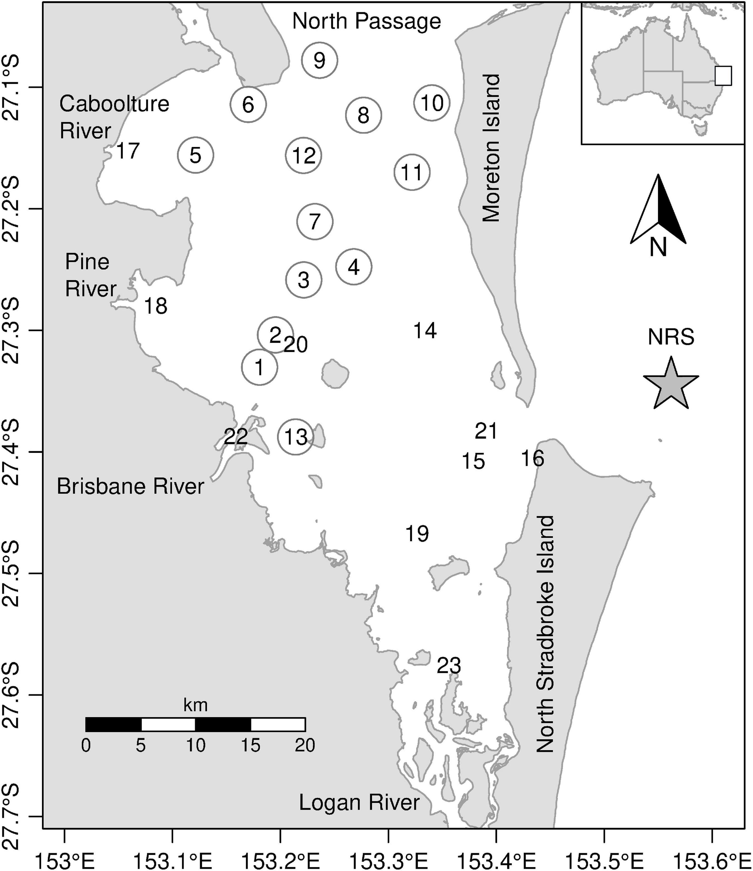
Figure 1. Map of station locations in Moreton Bay. Inset indicates location of Moreton Bay in Australia. Circled numbers indicate core stations sampled every trip and non-circled numbers are stations sampled occasionally. The star indicates the location of the IMOS National Reference Site mooring.
Materials and Methods
Study Site
Moreton Bay (27°15’S 153°15′E) is a shallow subtropical coastal embayment on the south-east Queensland coast (Figure 1). It covers an area of 1523 km2 and has an average depth of 6.8 m although areas of the bay north of the Brisbane River are approximately 30 m deep. It receives discharge from two major rivers (Brisbane and Logan) and several smaller ones (Dennison and Abal, 1999). The Brisbane River catchment (13,556 km2) together with that of the Logan River (3650 km2) and other small rivers (1823 km2) drains rural, agricultural, urban, and port areas. The seaward side of the bay is bordered by two large sand islands (Moreton and Stradbroke) that restrict the exchange of marine waters from the western Coral Sea with Moreton Bay. The main water exchange with the Coral Sea is via the 16-km wide North Passage. With an average evaporation of 1961 mm and an average annual rainfall of 1177 mm (Eyre and McKee, 2002; Wulff et al., 2011) within the Moreton Bay area, full strength salinity is generally retained throughout the bay for most of the year (Dennison and Abal, 1999; Quigg et al., 2010). Moreton Bay has a tidal range of 1.5–2 m with the central and northern sections of the bay flushed more than the southern and western sections. The average residence time in the bay is about 45 days (McEwan et al., 1998; Dennison and Abal, 1999), however the north east region near the North Passage is about 3–5 days. In this region, some proportion of the surface water flushed from Moreton Bay is often reintroduced as a deeper water intrusion on the following flood tides.
During periods of high discharge volume (>∼2 × 10⁶ ML), the Brisbane River can flow fresh to the bay (Davies and Eyre, 1998; Eyre et al., 1998). In addition, the Wivenhoe Dam, situated on the Brisbane River, 73 km from Moreton Bay (area 109 km2 and storage capacity of 3.132 million ML) can, during flood events release water from its storage capacity, extending the duration of the high volume of water flowing down the Brisbane River (Burford et al., 2012b; O’Brien et al., 2016). Between 2 and 6 weeks post flood, there was a major release of freshwater from Wivenhoe Dam from 21 February 2011, which led to salinity measurements at station 1, near the mouth of the Brisbane River, to be almost as low as those recorded 1-week post flood (Table 1).
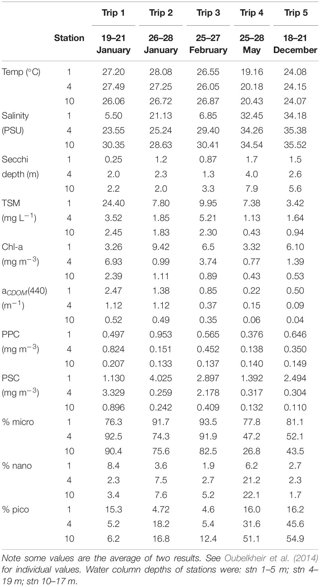
Table 1. Values of environmental parameters from surface water samples collected from three stations within Moreton Bay, I, 2, 6, 19, and 48-weeks post flood.
Major floods are classified as those where extensive low-lying areas next to the water course are inundated with water, causing evacuations of humans and animals and potential isolation of towns or cities. For the Brisbane River, which has a maximum baseline height of 1 m, a major flood is recorded when the river height exceeds 3.5 m. Since records began in 1841, there have been <10 occurrences of major flood events where the waters of the Brisbane River were measured to be higher than 4 m at the city gauge; the gauge closest to Moreton Bay. The last of these events occurred in January 2011, when the Brisbane River peaked at 4.46 m at 3 am on 13 January 2011 and was described, by flood forecasting models, as a “once in 100-year event.” As a result, enormous volumes of freshwater flowed from the Brisbane and other rivers into Moreton Bay, carrying with it, thousands of tonnes of sediment (Brown and Chanson, 2012; Steven et al., 2014; O’Brien et al., 2016), particulate and dissolved nutrients, CDOM and contaminants. This study is the first to provide a comprehensive study of the phytoplankton assemblage, using several complimentary techniques – microscopic analysis of phytoplankton abundance and species identification together with pigment concentration and composition and remote sensing satellite imagery – to track the effects of the flood event in Moreton Bay over a 12-month period.
Sampling Strategy
Immediately after maximum flood levels were reached and prior to the sampling program being established, satellite remote-sensed images showed a large flood plume flowing from the mouth of the Brisbane River, north along the western shore of Moreton Bay. To represent effects of the flood waters throughout Moreton Bay, sampling sites were chosen within the flood plume and at varying distances from the flood plume (Figure 1) and were sampled 1 (19–21 January), 2 (26–28 January), 6 (25–27 February), 19 (25–28 May), and 48 (18–21 December) weeks post flood. During the sampling at 6 weeks post flood, an additional three stations were sampled in south-east Moreton Bay, and during the 48-weeks post flood sampling a further three stations were sampled, close to the mouths of the Caboolture and Pine Rivers and in the south of Moreton Bay (Figure 1). At each site, samples were collected from the surface water for the analysis of phytoplankton pigments, phytoplankton cell counts (except 1 week post flood), Total Suspended Matter (TSM), and Colored Dissolved Organic Matter (CDOM). Samples for the analysis of nutrients and other bio-optical parameters, along with CTD profiles were also collected at each site (Oubelkheir et al., 2014).
Phytoplankton Pigments
A known volume of sample water was filtered through a glass-fiber filter (47 mm Whatman GF/F), which was then stored in liquid nitrogen until analysis. Samples were extracted over 15–18 h in an acetone solution before analysis by HPLC using a C8 column and binary gradient system with an elevated column temperature following the protocol described in Clementson (2013). Pigments were identified by retention time and absorption spectrum from a photo-diode array (PDA) detector and concentrations of pigments were determined from commercial and international standards (Sigma, United States; DHI, Denmark).
Pigment analysis is used to estimate algal community composition and concentration. Pigments which relate specifically to an algal class are termed marker or diagnostic pigments (Jeffrey and Vesk, 1997; Jeffrey and Wright, 2006). Some of these diagnostic pigments are found exclusively in one algal class (e.g., prasinoxanthin in prasinophytes), while others are the principal pigments of one class, but are also found in other classes (e.g., fucoxanthin in diatoms and some haptophytes; 19′-butanoyloxyfucoxanthin in chrysophytes and some haptophytes). The presence or absence of these diagnostic pigments can provide a simple guide to the composition of a phytoplankton community, including identifying classes of small flagellates that cannot be determined by light microscopy techniques. In this study, the description of the phytoplankton community composition is based on the pigments/algal groups listed in Table 2.
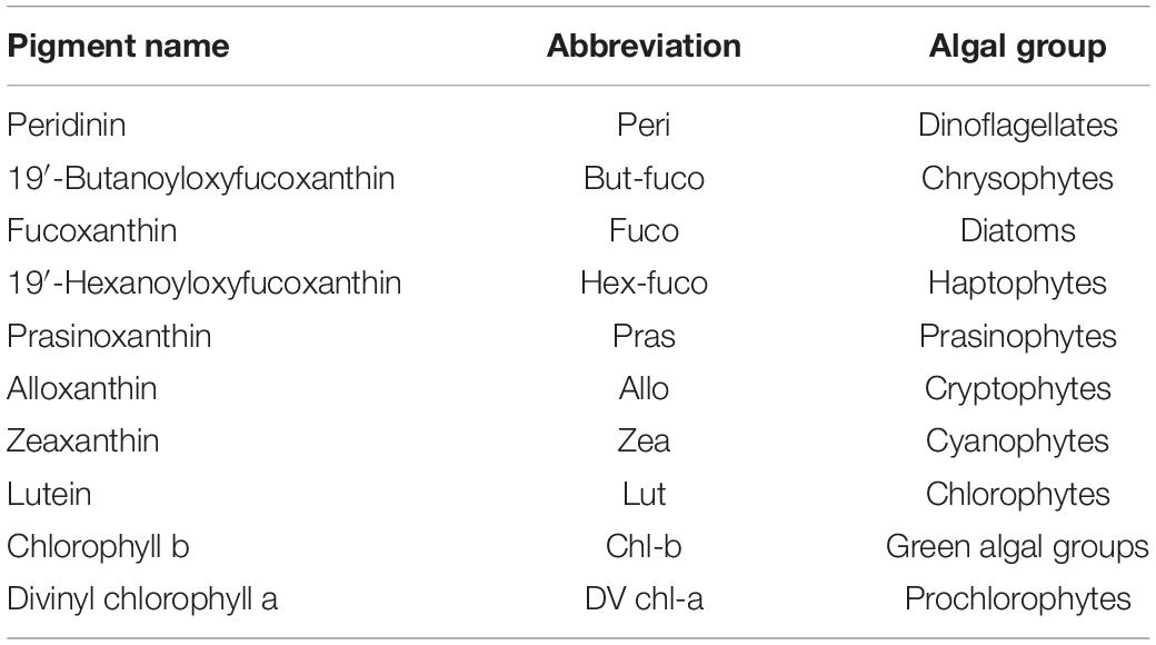
Table 2. Biomarker pigments and the algal groups they represent (Egeland et al., 2011).
Carotenoid accessory pigments can be described as either photosynthetic (PSC), those that transfer energy to reaction centers during photosynthesis or photoprotective (PPC), those that prevent damage to the chloroplast from high light conditions. In this study the concentration of PPC was the sum of violaxanthin, diadinoxanthin, alloxanthin, diatoxanthin, zeaxanthin, lutein, and carotenes, while the concentration of PSC was the sum of peridinin, 19′-butanoyloxyfucoxanthin, fucoxanthin, and 19′-hexanoyloxyfucoxanthin.
Diagnostic pigments can be used to determine the size class distribution of the phytoplankton community, based on established methods (Vidussi et al., 2001; Uitz et al., 2006). Size classes are micro (>20 μm), nano (2–20 μm), and picoplankton (< 2 μm).
Phytoplankton Identification and Abundance
Collected at the same time as the pigment samples during sampling trips 2–48 weeks post flood, phytoplankton samples were analyzed to determine cell abundance and identification of species. A surface water sample was collected in a 200 ml plastic bottle preserved using Lugol’s solution and stored at 4°C before concentrating using a sedimentation technique (Hötzel and Croome, 1999) to a final volume of 10 ml. Phytoplankton identification and enumeration (Tomas, 1997; Hallegraeff et al., 2010) to the lowest possible taxon was undertaken using a Leica DMLS standard compound microscope equipped with phase contrast (maximum magnification ×400). Phytoplankton abundance was estimated by counting up to 100 cells of the most dominant taxa using the Lund cell method (Hötzel and Croome, 1999). For some taxa, species-level identification was not possible using routine light microscopy and, in these instances, individuals were identified to genus level (e.g., Chaetoceros spp., Pseudo-nitzschia spp., and Thalassiosira spp.). Trichodesmium erythraeum filaments were converted to cell counts using a conversion factor (30 cells filament–1) that was obtained by averaging cell counts of 40 filaments (standard deviation, 6.4 cells filament–1). Cell biovolume was calculated on the geometric shapes and associated equations assigned for microalgae (Hillebrand et al., 1999).
Colored Dissolved Organic Matter
A known volume of sample water was filtered through a 0.22 μm filter (Millipore Durapore), and the filtrate was stored in clean dry glass bottles and kept cool and dark until analysis, generally within 24–72 h after collection. After equilibrating to room temperature, the CDOM absorbance of each filtrate was measured from 250 to 800 nm in a 10 cm pathlength quartz cell using a Cintra 404 UV/VIS spectrophotometer, with fresh Milli-QTM water (Millipore) as a reference. The CDOM absorption coefficient (aCDOM(l), m−1) was calculated using the equation aCDOM = 2.3(A(λ)/l) where A(λ) is the absorbance (normalized to zero at 680 nm) and l is the cell path length in meters. Finally, to smooth the scan, an exponential function was fitted to the CDOM spectra over the wavelength range 350–680 nm.
Total Suspended Matter
A known volume of sample water was filtered through a pre-weighed glass-fiber filter (47 mm Whatman GF/F) that had been previously muffled at 450°C. The filter was then rinsed with ∼ 50 ml of distilled water to remove any salt from the filter and dried to constant weight at 65°C to determine the TSM.
Remote Sensing
Remotely sensed CDOM absorption based on MODIS satellite imagery was used to map the spatial extent of flood waters into Moreton Bay. MODIS derived CDOM has been shown to be an effective surrogate for salinity (Schroeder et al., 2012) and in the case of the 2011 Moreton Bay floods, Oubelkheir et al. (2014) showed that in situ CDOM and salinity were highly inversely correlated, therefore allowing CDOM to be used or interpreted as a surrogate for salinity. This technique uses a physics-based ocean color inversion algorithm to derive CDOM absorption from MODIS satellite observations, which is then subsequently converted into salinity using an empirical relationship derived from linear regression of in situ CDOM and salinity measurements. The physics-based inversion algorithm outlined in Schroeder et al. (2012) was used to map the spatial extent of CDOM absorption in Moreton Bay during or close to the field observation periods (Figure 2).
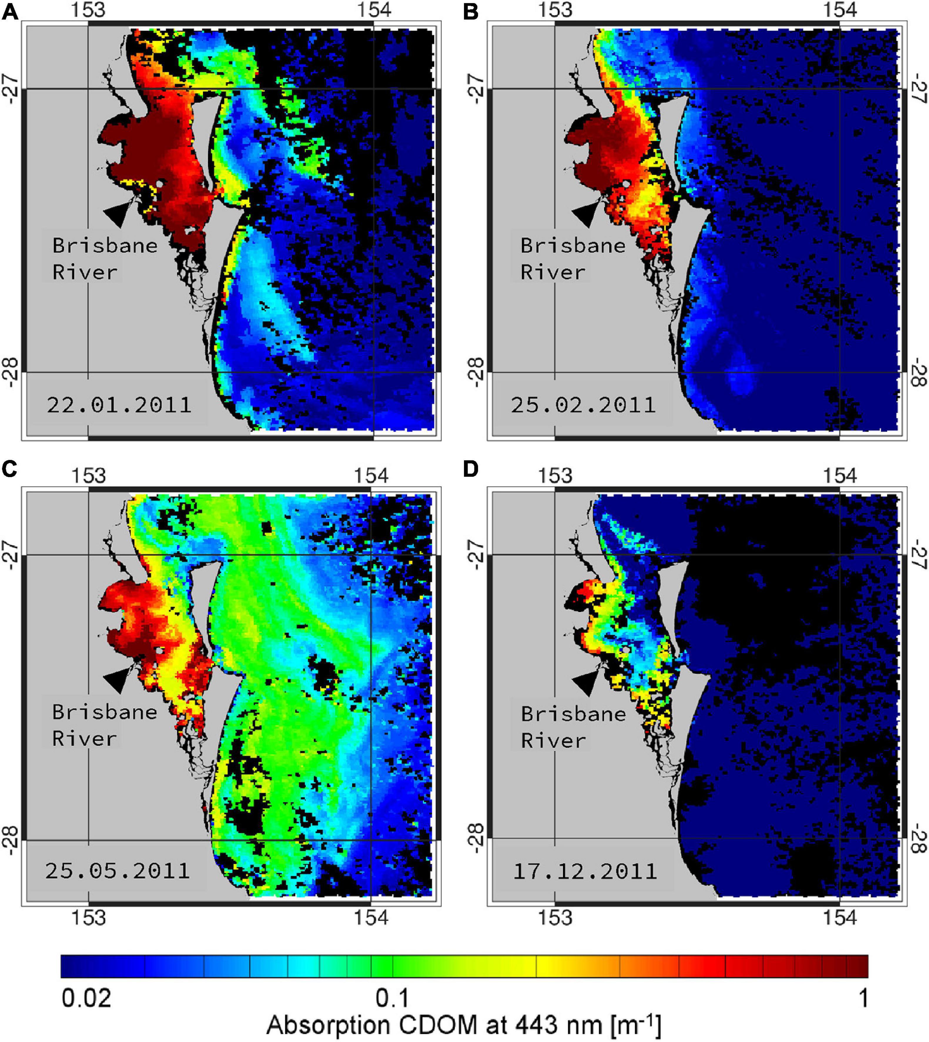
Figure 2. Sequence of remotely sensed images of CDOM absorption at 443 nm from MODIS observations covering Moreton Bay on 22 January, 25 February, 25 May, and 17 December 2011.
MERIS Level 2 Full Resolution Full Swath product that were largely cloud-free over Moreton Bay were downloaded from ESA MERCI (https://merisfrs-merci-ds.eo.esa.int/merci/) and Chl-a (algal 2 product for Case II waters based on a neural network algorithm) were obtained. Errors in Chl-a obtained in other estuarine-shelf waters using the neural network algorithm were similarly corrected using an adaptive algorithm (Liu et al., 2021). In situ HPLC obtained during trip 3 (24–27 Feburary 2011, 18 stations), trip 4 (26–27 May 2011, 14 stations), and trip 5 (17–20 December 2011, 14 stations) were used to calibrate MERIS algal 2 Chla products acquired on 26 February, 24 May, and 20 December. Maximum time interval between in situ data and satellite data was 2 days. A comparison of Chl-a values extracted from the algal 2 product with in situ HPLC Chl-a were highly overestimated (up to three times) in Moreton Bay (Figure 3B). Therefore, based on the relationship between field-measured and the algal 2 estimated Chl-a (y = 0.26 × x + 0.27, R2 = 0.63, Figure 3B), the algal 2 product was further calibrated to obtain more accurate MERIS-derived Chl-a for Moreton Bay by subtracting the intersect and dividing by the slope. Subsequently, a long time-series of calibrated MERIS-Chl-a were generated for the period before and after the extreme flood event (October 2010–December 2011; Figure 3A). Mean Chl-a values (averaged for field sampling sites; Figure 3C) were then extracted for Moreton Bay.
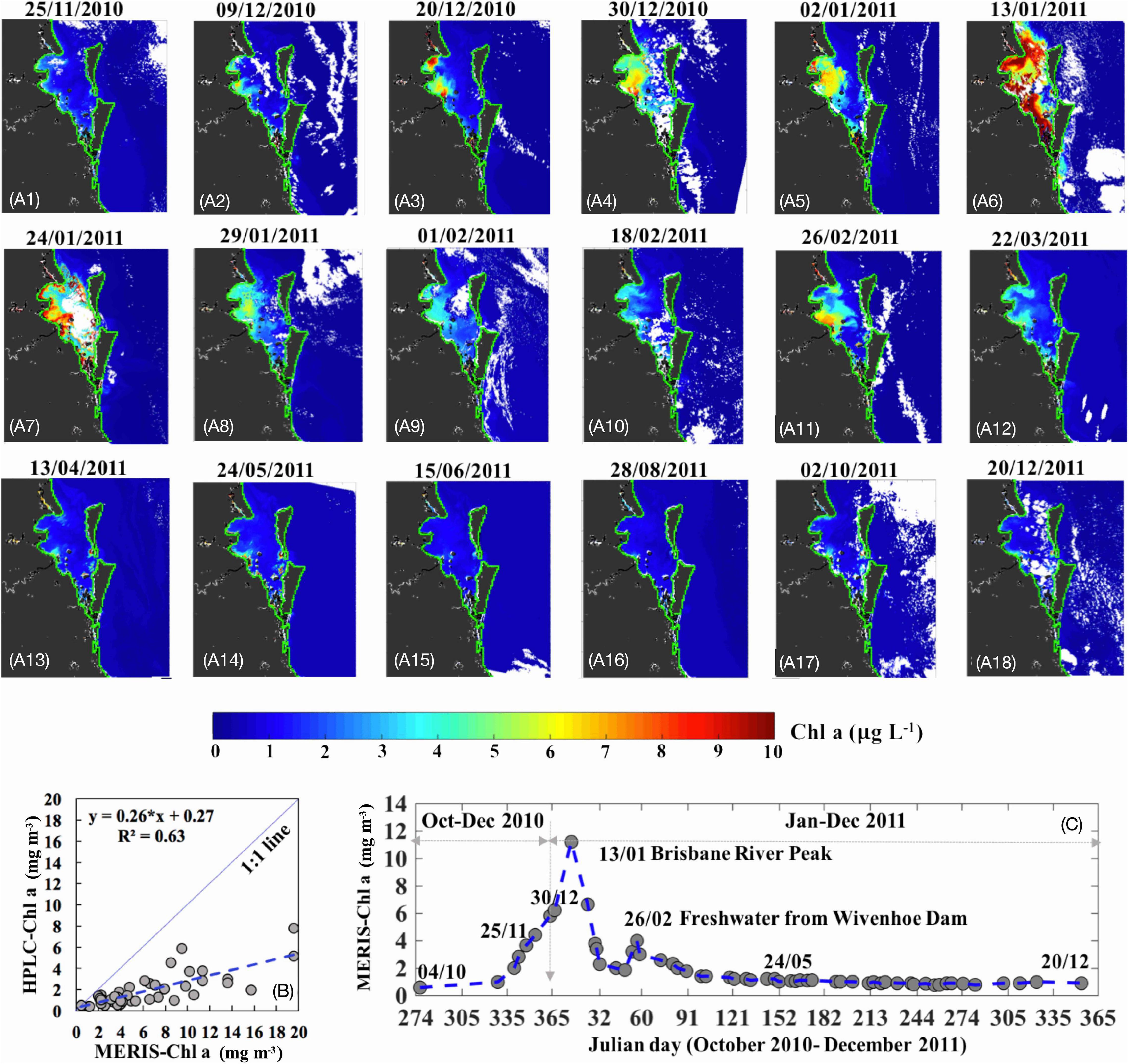
Figure 3. (A1–18) MERIS-derived Chl-a shown for the period of 25 November 2010 to 20 December 2011. (B) Relationship between MERIS neural network Chl-a (algal 2 product for Case 2 waters) and in situ HPLC-Chl-a used for obtaining the corrected MERIS Chl-a (n = 46, p < 0.001). (C) Mean of Chl-a corresponding to locations of field sampling stations for ∼50 cloud-free MERIS images.
Based on the MERIS calibrated Chl-a and estimated phytoplankton absorption coefficients (aphy), a total of 22 phytoplankton pigments were retrieved by decomposing aphy using a non-negative least square (NNLS) algorithm (D’Sa et al., 2019; Liu et al., 2019). The NNLS-retrieved Chl-a, though slightly overestimated, was spatially highly correlated (R2 = 0.96), with the calibrated MERIS-Chl a (Figure 4A). Five important biomarker pigments including fucoxanthin (fuco), peridinin (peri), zeaxanthin (zea), alloxanthin (allo), and Chl-b retrieved from the NNLS algorithm agreed reasonably well with corresponding HPLC pigments (Figures 4A–F) and had p-values of <0.001. The overall overestimations of biomarker pigments could be attributed to uncertainties in the calibrated MERIS-Chl a and to the time differences (up to 2 days) between satellite and field data. Post flood spatiotemporal maps of biomarker pigments associated with specific phytoplankton groups were obtained over Moreton Bay.
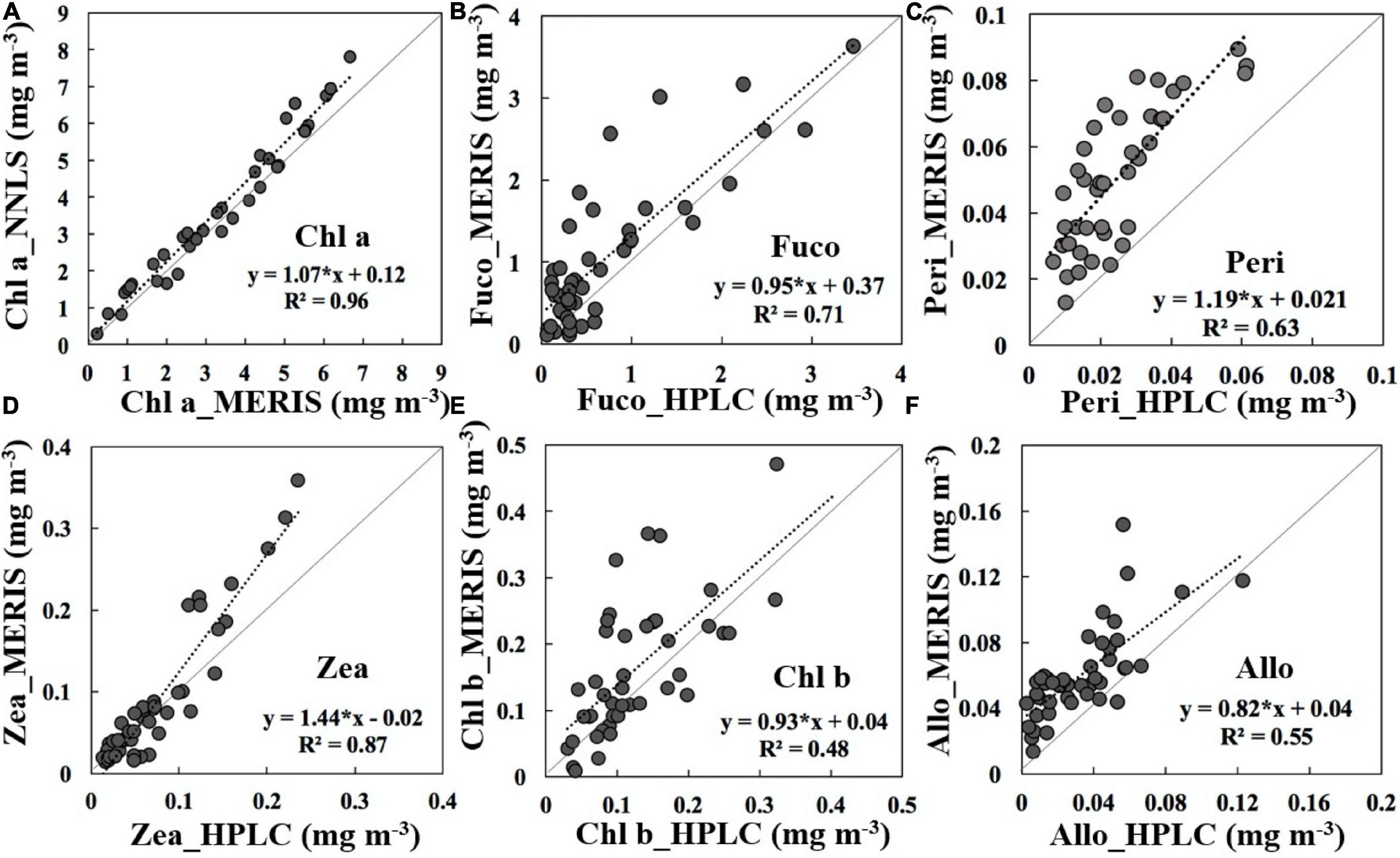
Figure 4. Comparisons of MERIS-derived versus HPLC measured pigment concentrations from the 6, 19, and 48 week post-flood sampling trips in Moreton Bay: (A) Chl-a, (B) fucoxanthin (fuco), (C) peridinin (peri), (D) zeaxanthin (zea), (E) Chl-b, and (F) alloxanthin (allo). For all plots n = 46 and p < 0.001. Refer to Table 2 for taxonomic groups represented by these pigments.
Statistical Analyses
Variation in indicator pigment composition was summarized using principal components analysis (PCA). Data were available for 12 sites and 5 sampling trips. Pigment data were standardized by total chlorophyll a and square root transformed. To assess potential drivers of the community patterns, environment variables and size classes (estimated from pigments) were plotted as arrows on PCA plots using the envfit function of the R vegan package (Oksanen et al., 2019). With this method, the direction of an arrow for a variable is the direction that maximizes the correlation between the variable values of the samples and the (projected) locations of the samples along the arrow. Lengths of the arrows are proportional to the correlations. The envfit explanatory variables were checked for skewness and transformed as appropriate (arcsine for size class percentages; log for TSM and CDOM).
PCA was also used to summarize variation in phytoplankton species composition among sites and times. Data were available for 18 sites and for trips 2–5. Sites were sampled on 1–4 of these trips, but the majority were sampled on all four trips. For PCA, the phytoplankton community matrix was transformed with the fourth root and Hellinger transformations (Legendre and Legendre, 1998; Legendre and Gallagher, 2001). The fourth root transformation was applied to reduce asymmetry in abundance distributions and to focus the analysis on species assemblage rather than on abundant species (abundance varied over nearly three orders of magnitude).
Long Term Data Analyses
The Queensland Department of Environment (Ecosystem Health Monitoring Program – EHMP) have sampled several parameters from several sites within Moreton Bay on a regular basis since 1990. Monthly data for temperature, salinity, nitrogen concentration, and turbidity from 2002 to 2013 inclusively are presented in Supplementary Figure 1. Brisbane River flow data (Bureau of Meteorology) is presented as a time series (Supplementary Figure 2). Satellite retrieved estimates of CDOM absorption at 443 nm from a central location in Moreton Bay have been collected from 2002 to 2012 and presented as a time series as shown in Supplementary Figure 3.
Results
Bio-optical Parameters
The first clear image of Moreton Bay was obtained on 15 January 2011, just 2 days after the flood peaked (see Figure 3, Oubelkheir et al., 2014); the high spatial resolution Landsat-8 true color image showed the initial extent of the CDOM freshwater plume affecting the surface waters over a large proportion of the bay. The image shows the flow of freshwater, primarily from the Brisbane River, entering Moreton Bay and then flowing north, leaving the bay through the North Passage. Within a week, the MODIS image from 22 January 2011 showed that the freshwater plume was still affecting surface waters of the bay, but the very high aCDOM(440) values had receded toward the coast (Figure 2A). After a further 4 weeks, the image from 26 February 2011 showed highest CDOM absorption to be present around the mouths of the rivers flowing into Moreton Bay (Figure 2B). Three months later, the image from 25 May 2011 indicated CDOM absorption had reduced further with highest aCDOM(440) values isolated to an area around the mouth of the Brisbane River (Figure 2C). The image 11 months post flood (17 December 2011) indicated that surface waters over almost the entire bay were low in CDOM absorption; exceptions were two small areas along the coast that still showed elevated aCDOM(440) values (Figure 2D). In situ samples collected for CDOM analysis validate the extent of the plume as seen in satellite images (Table 1).
Results from 1-week post flood samples showed the January 2011 flood event had little effect on surface water temperatures of Moreton Bay (26–28°C). The extremely high values of all other parameters were likely to be only be a fraction of what would have been present in the bay immediately post flood.
The 2011 Flood Event
The flow of the Brisbane River has a moderate seasonal cycle, with stronger flows during the spring/summer period (September–March) and weaker flows during winter (June–August). Although there are periodic large rainfall events, the January 2011 flood event stands out as the most significant period in the time series (Supplementary Figure 2). During December 2010 and early January 2011, total rainfall in excess of 1000 mm was recorded in the Brisbane River catchment and in the 3 days prior to Brisbane River peaking on 13 January, the catchment had received rainfall in excess of 286 mm. At a gauging station on the Brisbane River, 131.1 km upstream of the river mouth, the mean daily stream flow was >625,000 ML d–1 (Saeck et al., 2013b). This volume of water was nearly four times more than flowed from the Brisbane River in the one in 20-year flood in 1996.
Other parameters show seasonal variation with a strong seasonality in temperature, and weaker seasonality in environmental conditions associated with sporadic event-driven floods during the spring, summer, and autumn (Supplementary Figure 1). Continuous temperature and salinity data have been recorded since 2009 at a site outside the eastern edge of Moreton Bay, 38 km from the Brisbane River mouth (Figure 1, IMOS national reference station); the temperature-salinity sensor (WET Labs WQM), situated at 20 m in the water column, clearly recorded that the effects of the January 2011 flood extended this far east around 10 days after the flood peaked (Supplementary Figure 4).
Strong spatial gradients in several environmental parameters were observed following the flood and became much weaker during other sampling trips (Figure 5). Across bay gradients for environmental parameters measured at three stations (1 – near mouth of the Brisbane River, 4 – mid-bay, and 10 – seaward edge of the bay near Moreton Island) and for each sampling trip are listed in Table 1. As seen in other studies (Clementson et al., 2004;Schroeder et al., 2012), CDOM and salinity demonstrate a conservative relationship with the highest aCDOM(440) value being recorded at station 1, the site of lowest salinity (Table 1 and Figure 8 in Oubelkheir et al., 2014). One-week post flood, Chl-a concentration (as an indicator of phytoplankton biomass) was highest mid-bay and results clearly indicated a transitional effect of the flood plume from west to east across the bay (Figure 5 and Table 1).
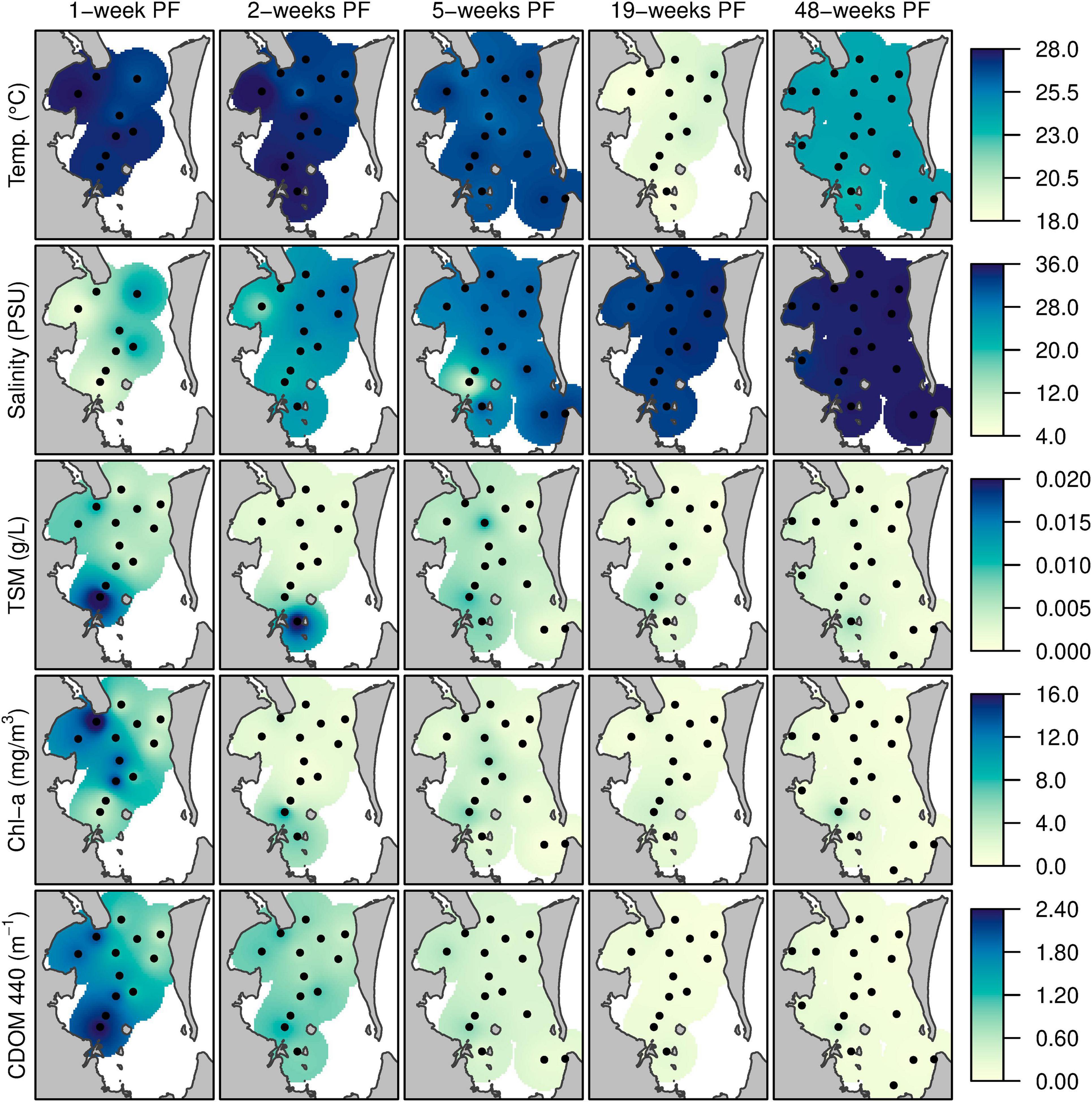
Figure 5. Maps of temperature, salinity, TSM, Chl-a concentration, and CDOM absorption coefficient surface properties across Moreton Bay 1-, 2-, 5-, 19-, and 48-weeks post flood: Maps were produced with inverse distance weighted averaging using the R gstat package, ignoring coastline topography (Pebesma, 2004).
Two weeks post flood, salinity had increased at most stations, but was still relatively fresh close to the mouth of the Brisbane River and the area of high TSM and CDOM was now restricted close to the river mouths, while Chl-a concentration had decreased at all stations (Figure 5 and Table 1). The effect of the release of freshwater from Wivenhoe Dam from 21 February 2011 was localized to stations close to the western shore of the bay (Figure 5), indicating that although the volume released was significant the flow was not strong enough for the freshwater to impact the surface waters of stations mid-bay and on the eastern side (Table 1 and Figure 5). Interestingly, the freshwater released from Wivenhoe Dam did not have the same content of CDOM as the flood waters 6 weeks previously as indicated by the aCDOM(440) value at station 1, 6 weeks post flood, being approximately a third of the value recorded during sampling trip 1 week post flood at the same station.
Results from trip 4 (19-weeks post flood) are confounded by the trip being sampled during the late autumn/early winter compared to the other trips sampled during summer. Winter conditions in Moreton Bay would expect to have low river discharge, cooler water temperatures, and lower phytoplankton biomass. Results from 19 weeks post flood show the highest salinities throughout the bay since the flood event together with water temperatures of ≈20°C throughout the bay (Figure 5 and Table 1) which are slightly lower than the long-term mean values for both parameters during May (Supplementary Figure 1). In addition, Secchi depth had deepened and aCDOM(440) values had reduced significantly at all stations (Table 1 and Supplementary Figure 1). Nearly 1 year past the peak flood period, temperature and salinity values across the bay were consistent with those observed for December over the long term (Table 1 and Supplementary Figure 1) and were the highest recorded post flood. The TSM value at the mouth of the Brisbane River (site 1) was the lowest post flood and aCDOM(440) values across the bay were the lowest observed, during field trips, post flood. After a period of warmer weather between field trips 19 and 48 weeks post flood, phytoplankton biomass, as indicated by Chl-a concentration, had increased at all sites (Figure 5 and Table 1).
Mean Chl-a values generated from MERIS images from October 2010 to December 2011 provided an overview of phytoplankton biomass at a greater temporal scale and showed a steady increase by December 2010 (Figures 3A,C) corresponding to increased rainfall and river discharge through December 2010.
A few relatively clear January 2011 images indicated peak mean Chl-a on 13 January 2011 (≈10.2 mg m–3; Figures 3A,C) corresponding to the peak Brisbane River discharge, and was higher than the mean in situ Chl-a obtained a week later (19–21 January 2011; ≈8.5 mg m–3) coinciding with the sampling trip, 1 week post flood. Moderate Chl-a values (≈6.5 mg m–3; Figure 3A6) in the Brisbane River plume waters (RGB imagery on 13 January 2011; not shown) appeared light limited due to high concentrations of TSM and CDOM (Figures 2, 3). Mean Chl-a decreased to ≈5.9 mg m–3 on 24 January (Figure 3A7), 3 days after the first field trip, with higher Chl-a values (≈9.8 mg m–3) observed at the Brisbane River mouth that subsequently decreased to lower values (≈2.2 mg m–3; Figure 3C) throughout the Bay until late February (Figures 3A8–10). However, a smaller Chl-a peak (≈4.5 mg m–3; Figure 3C) with highest levels at the Brisbane River mouth (≈9.2 mg m–3; Figure 3A11) and lower values around station 10 (≈1.0–1.5 mg m–3; Figure 3A11) was observed on 26 February 2011 that appeared to be stimulated by the release of freshwater from Wivenhoe Dam on 21 February 2011. Mean Chl-a returned to background levels (1.2 mg m–3; Figure 3C) in April 2011 and remained at those levels through May into December.
Phytoplankton Pigments
Pigment analysis from stations 1 (outside the mouth of the Brisbane River), 4 (mid-bay), and 10 (seaward edge of bay) in Moreton Bay showed similar pigment composition for trips 1–6 weeks post flood, with diatoms (as indicated by the presence of fucoxanthin) the dominant algal group at all three sites (Figure 6A). However, by 19 weeks post flood in May 2011, the composition had started to change, with a greater biomass of prasinophytes (prasinoxanthin), chlorophytes (lutein and Chl-b), cryptophytes (alloxanthin), and haptophytes (hex-fuco) present at each site than had been previously seen since the flood period. There was a west to east gradient across the bay, with least difference at station 1 and greatest difference in composition at station 10. The presence of divinyl Chl-a (DV Chl-a) at stations 4 and 10 at 6 weeks post flood, indicated the presence of Prochlorococcus spp. from an intrusion of more tropical water, from the north into Moreton Bay. By December 2011, nearly a year post flood, the proportion of diatoms, as indicated in the pigment composition, had significantly decreased compared to 1-week post flood. Again, there was a strong west to east gradient across the bay with species of green algae (prasinoxanthin, lutein, and chlorophyll-b) and probably Synechococcus sp. (zeaxanthin) more dominant at stations 4 and 10 than station 1.
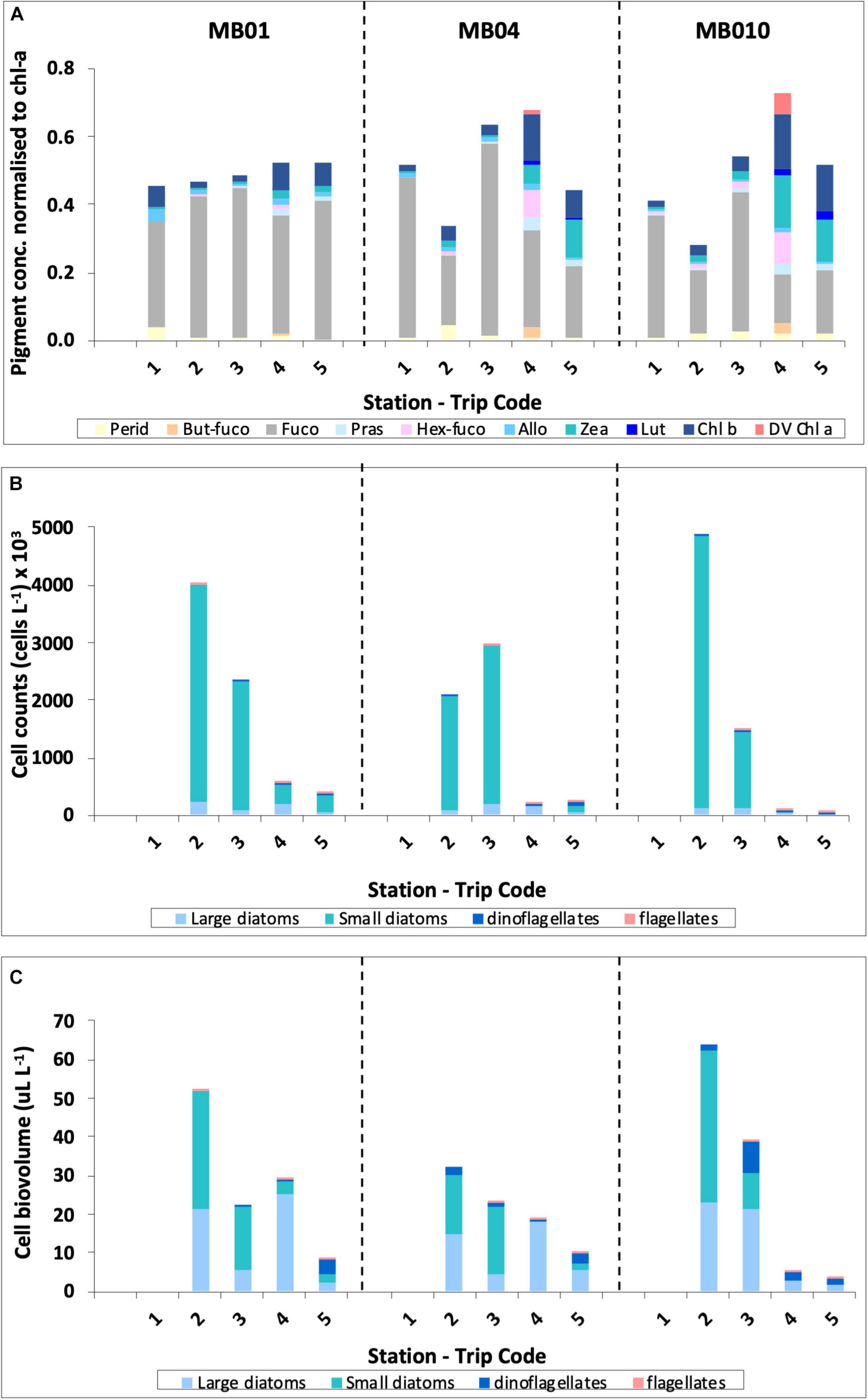
Figure 6. Phytoplankton composition in the surface waters of Moreton Bay during the five sampling trips post flood as indicated by: (A) pigment composition, (B) Phytoplankton cell counts, and (C) Phytoplankton cell counts adjusted for biovolume.
The NNLS-estimated phytoplankton biomarker pigments from MERIS agreed with the analysis of in situ pigment samples, adding a greater understanding of the spatial distribution. Corresponding to the peak discharge on 13 January and the highest mean satellite Chl-a observed over the Bay (Figure 3C), fucoxanthin was the dominant pigment with relatively high concentrations (>4 mg m–3; Figure 7A1) compared to the other four biomarker pigments (Peri, zeax, allo, and Chl-b). The distribution of fucoxanthin was highly and positively correlated with Chl-a, indicating the dominance of diatoms in response to the flood event. Chl-b (green algae) and allo (cryptophytes) were relatively low compared to fucoxanthin (Figures 7C1,E1) and zeaxanthin (cyanobacteria) showed extremely low concentrations across the bay (≈0.02 mg m–3; Figure 7D1). By 24 January, 10 days following the peak discharge, all biomarker pigments declined across Moreton Bay except for zeaxanthin. The pigments fucoxanthin (Figure 7A2), Chl-b (Figure 7C2), and alloxanthin (Figure 7E2) showed similar distributions with Chl-a, with maxima observed adjacent to the Brisbane River mouth. In contrast, peridinin (Figure 7B2) and zeaxanthin (Figure 7D2) displayed complementary patterns and were much lower near the Brisbane River mouth but highest in the north west of the bay close to the Caboolture River. On February 26, 5 days after freshwater outflows from Wivenhoe Dam, a second but smaller scale phytoplankton bloom was observed near the Brisbane River mouth (Figure 3A11). Pigment maps confirmed higher fucoxanthin (≈3.4 mg m–3) and hence diatom dominance at this site (Figure 7A3). Peridinin showed a similar distribution to fucoxanthin with a slight increase near the Brisbane River mouth (≈0.06 mg m–3; Figure 7B3), while Chl-b (≈0.16 mg m–3; Figure 7C3) and alloxanthin (≈0.05 mg m–3; Figure 7E3) decreased across the bay and zeaxanthin (Figure 7D3) showed minimum values around the Brisbane River mouth. Pigment maps for May 2011 showed lower levels of fucoxanthin (Figure 7A4), and peridinin (Figure 7B4) throughout Moreton Bay and in contrast, Chl-b (Figure 7C4) and zeaxanthin (Figure 7D4) increased over all the bay. Nearly 1-year post flood, the pigment maps showed a large increase in zeaxanthin (>0.1 mg m–3) across Moreton Bay while other pigments decreased (Figures 7A5–E5), suggesting the dominance of cyanobacteria species at this time.

Figure 7. MERIS-derived maps of diagnostic pigment concentrations for Moreton Bay. Simulated (A1–A5) fucoxanthin, (B1–B5) peridinin, (C1–C5) Chl-b, (D1–D5) zeaxanthin, and (E1–E5) alloxanthin. Vertical panels 1–5 represent maps for 13 January (1-week post flood), 24 January (2-weeks PF), 26 February (5-weeks PF), 24 May (19-weeks PF), and 20 December 2011 (48-weeks PF), respectively and horizontal panels (A–E) represent the different pigments; note the different concentration scale for each pigment.
Variation in the ratios of photoprotective carotenoids (PPC) to photosynthetic carotenoids (PSC) are strongly correlated to temperature and irradiance (Eisner and Cowles, 2005) and tend to increase in warmer, more nutrient deplete waters. Post flood 1, 2 and 6 weeks, the concentration of PSC was greater than PPC at all sites across the bay (Table 1). By 19-weeks post flood, during winter conditions, the PSC concentration was still greater than PPC at sites on the western edge and mid-bay, while at sites on the eastern edge the concentration of PSC and PPC were similar (Table 1). Nearly 1-year post flood, PPC concentration was greater than PSC at all sites except those close to the mouths of rivers (Table 1). PSC consist of pigments associated with diatoms, dinoflagellates, and haptophytes, while PPC consist of pigments associated with cryptophytes, green algae, and cyanobacteria.
Phytoplankton Cell Counts and Identification
The species were separated into 4 groups – large diatoms (>10 μm), small diatoms (<10 μm), dinoflagellates, and flagellates (Figures 6B,C). Light microscopy techniques, as used in this study, are limited to identifying phytoplankton species whose size is greater than about 8–10 μm. However, the microscopy and pigment data complement each other to deliver a total picture of the phytoplankton community composition to class level. Cell count data showed that during trips 2 and 3, small diatoms were the most abundant group throughout the bay (Figure 6B) and when the counts were adjusted for biovolume, a combination of large and small diatoms dominated the community composition at all sites (Figure 6C). By trip 4, in May 2011, the community at all sites across the Bay were dominated by large diatoms, while at site 10, on the eastern edge of the Bay, although large diatoms dominated, flagellates showed a stronger presence than at sites on the western edge or mid-bay (Figure 6C). Trip 5, nearly one-year post flood, flagellates were present at all sites across the Bay (Figure 6C).
Principle Component Analysis
The PCA of indicator pigments showed that, the first two axes explained 61% and 16% of the variance in the community matrix respectively (Figure 8). The first axis was correlated with time since flooding and the second axis correlated with season (winter to summer). On the first axis, trip 3 (19 weeks PF) samples tended to be located to the left of trip 2 (6 weeks PF) samples probably as a result of the post-flood Wivenhoe Dam release which occurred just prior to trip 3 and pushed some water properties back toward those of trip 1 (Figure 5).
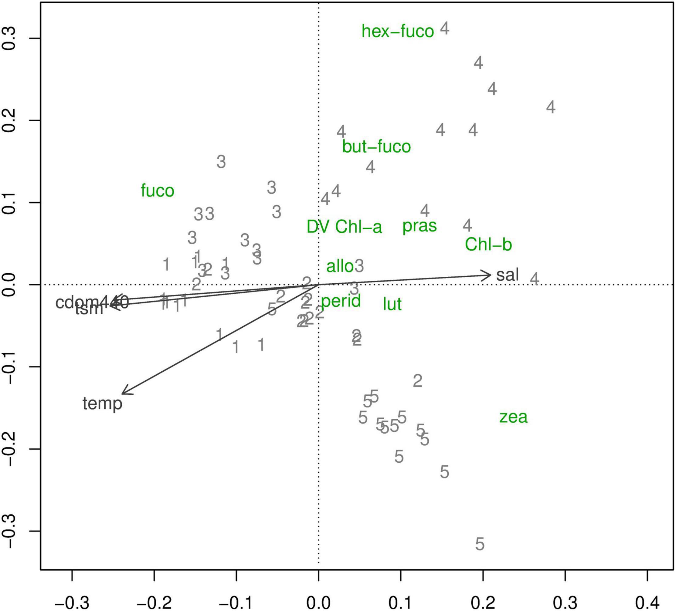
Figure 8. Principal components analysis of indicator pigments by trip. PCA sample scores are plotted as trip numbers. Species scores are plotted as pigment codes. The arrows indicate environment variables. Refer to Table 2 for full names of the pigments and the taxonomic group they indicate.
On the first axis, the only pigment showing a positive association with flooding was fucoxanthin (fuco), while pigments positively associated with non-flooding included zeaxanthin (Zea) and Chl-b (Figures 8 and 9). On the second axis, the pigments associated with winter were 19′-hexanoyloxyfucoxanthin (Hex-fuco) and 19′-butanoyloxyfucoxanthin (But-fuco), while zeaxanthin was the only pigment associated with the summer direction of that axis (Figures 8 and 9). Because the PCA axes were related to trip, the relationships between the PCA sample scores and environment variables were consistent with the relationships between environment variables and trip.
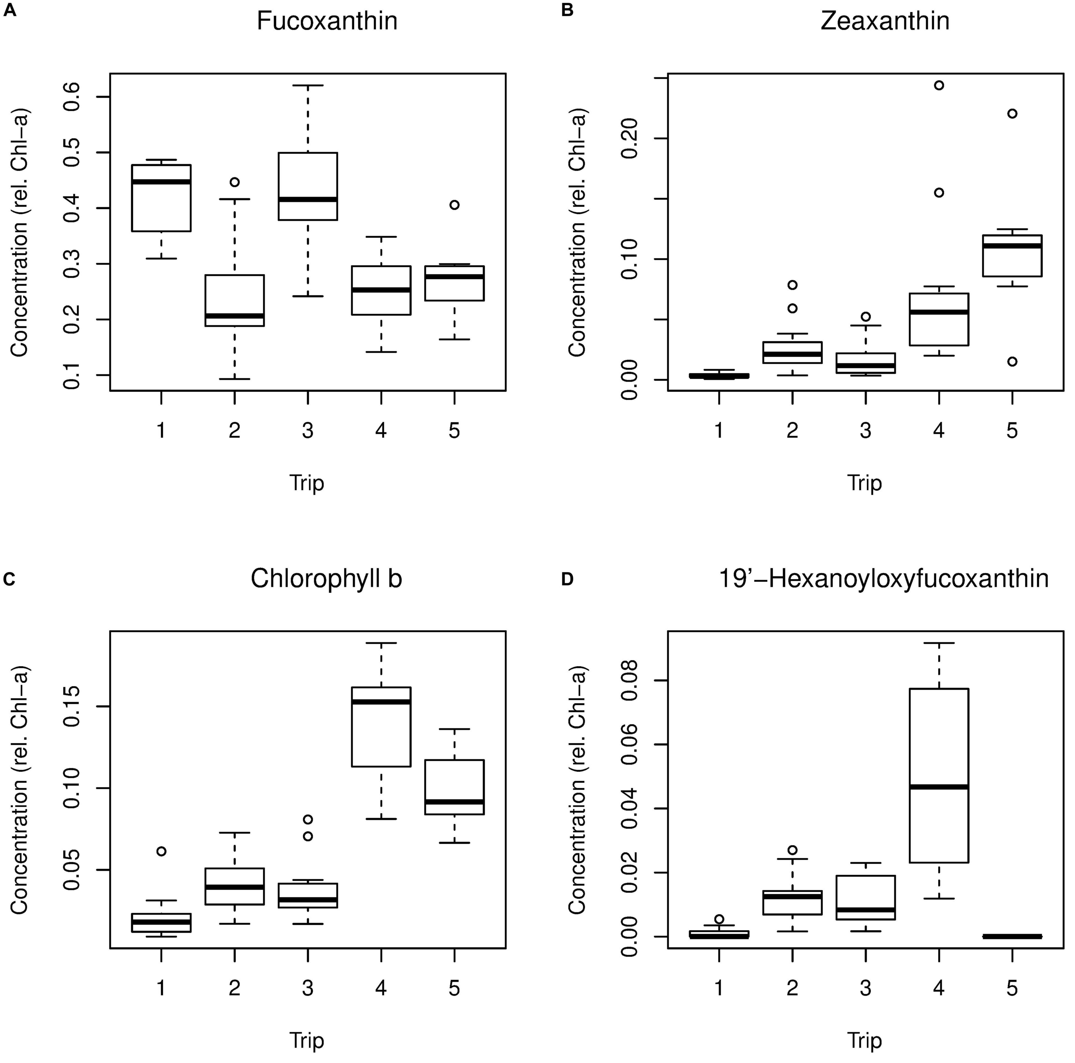
Figure 9. Boxplots showing variation in selected pigments by trip; (A) Fucoxanthin, (B) Zeaxanthin, (C) Chlorophyll b and (D) 19’-hexanoyloxyfucoxanthin.
Species composition observed during sampling trips 2 and 6 weeks post flood was associated with higher values of all environment variables except salinity, which was lower during trips 2 and 3 (Figure 10). In the phytoplankton PCA, the first two PCA axes explained 17% and 9% of the variance in the community matrix respectively; the first axis separated the two earlier trips 2 and 3, from the later trips 4 (6 weeks PF) and 5 (48 weeks PF), while the second axis separated trips 2 and 3 from one another (Figure 10). Diatoms were the phytoplankton group that was most associated with both trips 2 and 3; trip 2 included the smaller diatoms, Chaetoceros spp., while those associated with trip 3 included the larger Chaetoceros spp., Asterionellopsis glacialis, and Skeletonema spp. (all sizes) (Figures 10 and 11). Those associated with trips 4 and 5 were dinoflagellates Gymnodinium spp., Gyrodinium spp., and a silicoflagellate Octactis octonaria.
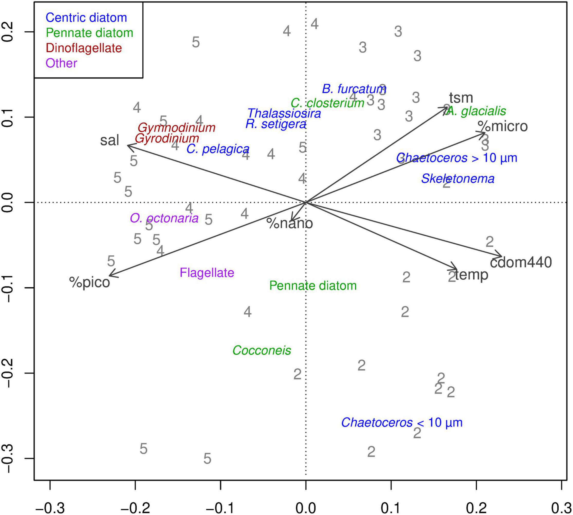
Figure 10. Principal components analysis of phytoplankton species by trip. PCA sample scores are plotted as trip numbers. Species scores are plotted as species names. The arrows indicate environment variables.
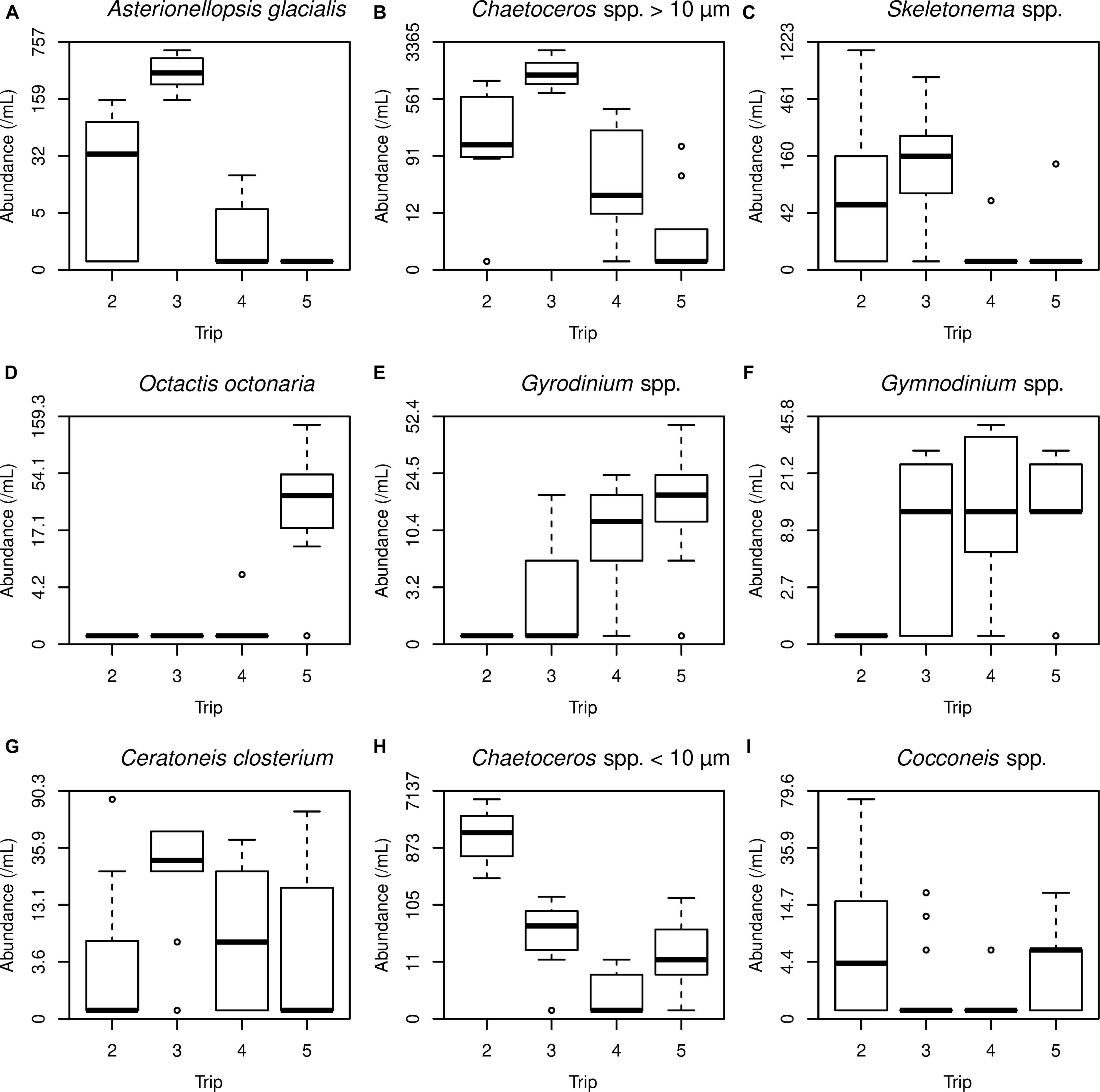
Figure 11. Boxplots showing variation in selected phytoplankton species by trip. The graphs are ordered according to PCA species scores: PCA1 positive (A–C), negative (D–F); PCA2 positive (G), negative (H, I). For example, A. glacialis was more abundant on trips 2 and 3, whose samples were mostly positive on PCA1.
Because the PCA axes were related to trip, the relationships between the PCA sample scores and environment variables (Figure 10) were consistent with the relationships between the environment variables and trip. Species composition in the earlier trips was associated with higher CDOM, TSM, temperature, and microphytoplankton (plankton > 20 μm) (Figure 10). That of the later trips was associated with higher salinity and picophytoplankton (plankton < 2 μm). The association of TSM with trip 3 is consistent with the post-flood release from Wivenhoe Dam, which began just before that field trip.
Discussion
Phytoplankton community composition in Moreton Bay was first recorded in 1954 (Wood, 1954), but there were few further studies until the 1990’s. Routine monitoring of chlorophyll-a (Chl-a) concentration and other biogeochemical parameters has taken place routinely throughout different sections of the bay (Department of Environment), while a one in 20 year flood in May 1996 initiated a series of studies. In some of these studies only concentrations of Chl-a were measured as an indicator of total phytoplankton biomass (Moss, 1998; Uwins et al., 1998), whilst other studies utilized microscopic analyses to measure phytoplankton abundance (Heil et al., 1998a, b). Further studies have reported estimates of primary production for Moreton Bay (O’Donohue and Dennison, 1997; O’Donohue et al., 2000; Glibert et al., 2006; Quigg et al., 2010; Saeck, 2012) and suspended sediment loadings during flood events (Davies and Eyre, 1998; Eyre et al., 1998; Brown and Chanson, 2012).
Based on a combination of remote sensing, algal pigment analysis, cell counts, and the ratios of PPC:PSC, this study found that the January 2011 flood event resulted in broad scale and rapid changes in the phytoplankton community in Moreton Bay. In the first few weeks after the event, the phytoplankton community was dominated by microplankton, principally diatoms. Immediately after the flood, smaller species of Chaetoceros spp. dominated, but later larger diatom species dominated (Chaetoceros spp., Asterionellopsis glacialis, and Skeletonema spp.). Globally, diatoms commonly dominate in coastal waters after large flood events (Schaeffer et al., 2012; Chakraborty and Lohrenz, 2015; Dorado et al., 2015). A previous study in Moreton Bay during a much smaller flood event, in May 1996, also showed diatoms – Rhizosolenia setigera, Pseudonitzschia sp., and Skeletonema costatum – dominating the phytoplankton composition (Heil et al., 1998a, b). Other studies in tropical Australia have shown that the diatoms, Chaetoceros spp., Skeletonema sp., Navicula sp., and Thalassionema nitzschioides can also dominate in coastal waters during floods (Howley et al., 2018).
After 19-weeks post flood, the phytoplankton community continued to be dominated by diatoms near the river mouth, but nanoplankton had become more dominant further from the mouth, i.e., prasinophytes, haptophytes, cryptophytes, and chlorophytes. The picoplankton fraction, dominated by cyanobacteria, also increased from an average value of 4% of the community composition at eastern and mid-bay sites 1 week post flood, to an average of 44%, 48 weeks post flood, indicating that under non-flood conditions, picoplankton is an important component of the phytoplankton community composition at most sites in Moreton Bay. Results from this study confirm the suggestion by Quigg et al. (2010) that cyanobacteria is a significant component of the phytoplankton community in Moreton Bay. PPC:PSC ratios were low at eastern and mid-bay sites 1-week post flood, indicating the flood plume affected the whole bay, and then generally increased at all sites, except those near the mouths of rivers, throughout the duration of the study.
Flood events can deliver increased dissolved inorganic nutrient concentrations to estuaries and bays which phytoplankton are capable of rapidly using. However, accompanying high values of TSM and CDOM absorption reduce light penetration, which may reduce phytoplankton growth rates. On the leading edge of the plume, and with distance from the river mouth, particulate loads will descend to deeper in the water column, and CDOM concentration will be diluted, allowing light penetration to increase and phytoplankton in these regions to take advantage of the increased nutrient concentrations. It has previously been suggested that the location where this takes place in any system is at mid-salinities where the TSM concentration falls below 10 mg L–1 (Dagg et al., 2004). In this study, 1-week post flood, the highest values of phytoplankton biomass (as indicated by Chl-a concentration) were at mid-bay sites where salinity was about 26 PSU, and the TSM concentration was <10 mg L–1. Only the sites near the mouth of the Brisbane River had TSM concentrations > 10 mg L–1.
Changes in phytoplankton composition and the concentration of environmental parameters can be affected by the exchange of water in the bay with more oceanic water from the north. Models have shown this to be a complex matter in Moreton Bay (McEwan et al., 1998). The residence time of water in Moreton Bay, under non-flood conditions, ranges from 43 to 75 days with an average of 42 days (Saeck et al., 2019). The longer residence times are generally restricted to the southern region of the bay, south of the Brisbane River which was less affected by the flood plume than other regions of the bay. The region in the north-east of the bay, close to North Passage, has the shortest residence time of 3–5 days (Saeck et al., 2019). Despite this normally short flushing time, effects of the flood were recorded 10 days after maximum flood levels were reached, at a temperature/salinity sensor located in the Coral Sea off the north-east coast of North Stradbroke Island, some 38 km from the Brisbane River (Figure 1). Three extensive sampling trips completed in the 42 days post flood (average residence time) indicated that north/south and east/west gradients in both phytoplankton composition and environmental parameters existed and changed with time.
The flood generated a bottom-trapped type flood plume from the Brisbane River that flowed north along the western coastline, covered >500 km2 of Moreton Bay, was 15–25 m thick reaching the bottom in shallow waters, and took 3–4 weeks to disappear (Yu et al., 2014). The plume size was most strongly influenced by the Brisbane River discharge (R2 = 0.87) which had a peak flow of 620, 520 ML d–1. To put the scale of this event in perspective, the one in 20 year flood in May 1996 had a peak flow discharge of the Brisbane River of 169,797 ML d–1 (Saeck, 2012). The suspended sediment associated with this discharge was described as silt (Brown and Chanson, 2012) and based on suspended sediment concentrations, the quantity discharged to Moreton Bay was estimated to be of the order of 1 million tonnes (Steven et al., 2014). The Brisbane River catchment, during an average year, exports approximately 178,000 tonnes (Eyre et al., 1998). Recent studies have highlighted that suspended sediments are more important than previously thought as an immediate source of ammonium to stimulate phytoplankton growth (Franklin et al., 2018; Garzon-Garcia et al., 2018; O’Mara et al., 2019) and long term, silt deposition from flood events is filling the deeper basin of the Bay which will increase benthic-pelagic coupling (Coates-Marnane et al., 2016; Lockington et al., 2017).
Other studies have reported on flood events or time series of river discharge (Peierls et al., 2003; Muylaert and Vyverman, 2006; Chakraborty and Lohrenz, 2015; Dorado et al., 2015; Liu et al., 2019), but with the exception of the Amazon River no other study has reported on discharges into an estuary/bay system of the magnitude recorded for Moreton Bay in 2011. In Moreton Bay itself, the flood of 1996 was the previously most studied event and yet the values of all measured parameters after the flood were found to fall within the long term range of measurements observed during non-flood conditions (Moss, 1998) indicating the impact of the flood event on the phytoplankton community to be minimal. Since the 1996 flood, upgrades were made to the sewerage treatment plant (STP) near the mouth of the Brisbane River, reducing the annual nitrogen output from the STP to Moreton Bay by 70%. Flood discharges are now an important source of nutrients for a phytoplankton bloom to establish in the Bay (Saeck et al., 2013b).
Most similar to this study was that conducted in a subtropical estuary in the northern hemisphere – Galveston Bay in the Gulf of Mexico (Dorado et al., 2015). In this study discharge events were monitored for 22 months (February 2008 to December 2009) and significant events were considered to be any discharge >283 m3 s–1; in comparison, the Moreton Bay 2011 flood event had a discharge of 7182 m3 s–1. Despite the vast difference in the discharge magnitude, the observations in phytoplankton community composition were very similar; diatoms dominated at sites affected by high river discharge, while cyanobacteria dominated during periods of low discharge. Similar observations were reported for the northern Gulf of Mexico (Chakraborty and Lohrenz, 2015) and also for mesocosm experiments aimed at simulating the water conditions after a discharge (Paczkowska et al., 2020). The similarity between these studies and this study suggests that subtropical embayments are generally pico-dominated communities which can be disturbed by high discharge-events, but can recover; the recovery time is dependent on the discharge volume relative to the volume of the bay. The question for the future is, can these systems continue to recover if the frequency of discharge increases. Models predict an increase in high river flow in south-east Queensland for 2071–2100 relative to 1971–2000 (van Vliet et al., 2013).
The January 2011 flood event, described as a “once in one-hundred-year event,” would have had an immediate and dramatic effect on the phytoplankton community composition of Moreton Bay, causing extensive change to the ecosystem structure over a very short time scale. All parameters analyzed, both analytically and statistically, indicate that immediately after the flood event, the turbid and highly colored freshwater flowing into Moreton Bay provided an environment where microplankton – diatoms and dinoflagellates – flourished. Exactly when the effects of the flood event subsided is confounded by two events; the release of additional fresh water from the Wivenhoe Dam approximately 5-weeks post the initial flood peak and the change of seasons from summer into autumn/early winter which occurred between 6 and 19 weeks post flood. However, size class analysis clearly illustrates the transition of a microplankton dominated community, throughout the bay, immediately post flood to a community, throughout most of the bay, where picoplankton was dominant or at least an important component, during non-flood conditions. Without pre-flood time series of phytoplankton species in the bay, it is not possible to definitively determine whether the phytoplankton community composition in Moreton Bay was able to recover from the extreme flood event. However, monthly monitoring of other parameters in Moreton Bay (Supplementary Figure 1) and satellite retrieval of CDOM estimates for the 10 years preceding the flood (Supplementary Figure 3) did show recovery to pre-flood values. Other studies which have been based on routine phytoplankton monitoring (Chakraborty and Lohrenz, 2015; Dorado et al., 2015), have shown that subtropical embayments are generally dominated by picoplankton during periods of low river discharge and by microplankton during high river discharge.
If we assume the phytoplankton community within Moreton Bay behaves similarly to the communities in other subtropical bays, then it would seem that the phytoplankton in Moreton Bay exhibited resilience in being able to adapt and then recover from a 1 in 100-year flood event. However, if changing climate conditions cause severe floods to become more frequent, as is projected, it is unclear as to whether the Moreton Bay phytoplankton community could continue to be as resilient in the future. The length of this study has generated a detailed dataset that provides baseline data for both non-flood and flood conditions in Moreton Bay, which will be extremely useful for water quality management and assessing phytoplankton community change during future flood events. Implications for higher trophic levels and the water/atmospheric flux of carbon may arise, if the frequency of future flood events results in phytoplankton community composition changes from pico-dominated to nano- or micro-dominated over longer time scales.
To deal with the potential increased frequency in flood events and associated potential trophic changes, water quality management of Moreton Bay should include routine monitoring of phytoplankton at several sites within the bay. In addition, or at the least alternatively, water samples should be collected for the analysis of pigment composition and concentration, which will provide an indication of phytoplankton community composition to group level. A time series of this data will provide a baseline from which the level of recovery or resilience of the phytoplankton community can be assessed after a flood or other extreme weather event. This study is based on a single flood event, and as such our findings are suggestive rather than conclusive. Future work involving analysis of data from multiple flood events will provide more certainty about the primary drivers and consequences to the phytoplankton community of major flood events.
Data Availability Statement
The datasets presented in this study can be found in online repositories. The names of the repository/repositories and accession number(s) can be found below: All bio-optical data (pigment concentration, TSM concentration and absorption coefficients for phytoplankton, non-algal, and CDOM) together with phytoplankton cell count and abundance data can be found at (Clementson et al., 2020) https://doi.org/10.25919/gf5w-9711.
Author Contributions
LC led the project, analyzed the results, and wrote the first draft of the manuscript. AR provided support in the analysis and the writing of the manuscript. WR analyzed the results and provided first drafts of most figures. KO designed the field program and analyzed results. BL and ED developed a neural network algorithm and provided the data for Figures 3, 4 and 7. LG and PA analyzed the phytoplankton results. TS analyzed the CDOM remote sensing results. PF assisted in the field program implementation and analyzed the results. MB and ES provided data from complimentary projects and analyzed the data. AS provided support in the analysis and the writing of the manuscript. All authors contributed to the article and approved the submitted version.
Funding
Funding for this study was provided by the CSIRO Wealth from Ocean Flagship (ORCA). ED and BL acknowledge partial funding from NASA grant 80NSSC18K0177.
Conflict of Interest
The authors declare that the research was conducted in the absence of any commercial or financial relationships that could be construed as a potential conflict of interest.
Acknowledgments
We thank Sean Maberly, skipper of the FRV Tom Marshall (DEEDI) and Andrew Lowe skipper of the Mirrigimpa (DERM); Derek Fulton for assistance with the figures. We are grateful to Ruth Eriksen for the internal review and constructive comments of this paper. We would also like to thank NASA and the European Space Agency (ESA) for providing access to the MODIS and MERIS ocean color data respectively.
Supplementary Material
The Supplementary Material for this article can be found online at: https://www.frontiersin.org/articles/10.3389/fmars.2021.580516/full#supplementary-material
References
Alpine, A. E., and Cloern, J. E. (1992). Trophic interactions and direct physical effects control phytoplankton biomass and production in an estuary. Limnol. Oceanogr. 37, 946–955. doi: 10.4319/lo.1992.37.5.0946
Angeler, D. G., Alvarez-Cobelas, M., Rojo, C., and Sánchez-Carrillo, S. (2000). The significance of water inputs to plankton biomass and trophic relationships in a semi-arid freshwater wetland (central Spain). J. Plankton Res. 22, 2075–2093. doi: 10.1093/plankt/22.11.2075
Ansotegui, A., Sarobe, A., Trigueros, J. M., Urrutxurtu, I., and Orive, E. (2003). Size distribution of algal pigments and phytoplankton assemblages in a coastal–estuarine environment: contribution of small eukaryotic algae. J. Plankton Res. 25, 341–355. doi: 10.1093/plankt/25.4.341
Brown, R., and Chanson, H. (2012). Suspended sediment properties and suspended sediment flux estimates in an inundated urban environment during a major flood event. Water Resources Res. 48. doi: 10.1029/2012WR012381
Burford, M. A., Webster, I. T., Revill, A. T., Kenyon, R. A., Whittle, M., and Curwen, G. (2012a). Controls on phytoplankton productivity in a wet-dry tropical estuary. Estuar. Coast. Shelf Sci. 113, 141–151. doi: 10.1016/j.ecss.2012.07.017
Burford, M. A., Green, S. A., Cook, A. J., Johnson, S. A., Kerr, J. G., and O’Brien, K. R. (2012b). Sources and fate of nutrients in a subtropical reservoir. Aquat. Sci. 74, 179–190. doi: 10.1007/s00027-011-0209-4
Chakraborty, S., and Lohrenz, S. E. (2015). Phytoplankton community structure in the river-influenced continental margin of the northern Gulf of Mexico. Mar. Ecol. Progress Series 521, 31–47. doi: 10.3354/meps11107
Chan, T. U., and Hamilton, D. P. (2001). Effect of freshwater flow on the succession and biomass of phytoplankton in a seasonal estuary. Mar. Freshw. Res. 52, 869–884. doi: 10.1071/mf00088
Clementson, L. A. (2013). “The CSIRO method,” in The Fifth SeaWiFS HPLC Analysis Round-Robin Experiment (SeaHARRE-5). NASA Technical Memorandum 2012-217503, eds S. B. Hooker, L. A. Clementson, C. S. Thomas, L. Schlüter, M. Allerup, and J. Ras (Greenbelt, MD: NASA Goddard Space Flight Center), 98.
Clementson, L. A., Parslow, J. S., Turnbull, A. R., and Bonham, P. I. (2004). Properties of light absorption in a highly coloured estuarine system in south-east Australia which is prone to blooms of the toxic dinoflagellate Gymnodinium catenatum. Estuar. Coast. Shelf Sci. 60, 101–112. doi: 10.1016/j.ecss.2003.11.022
Clementson, L., Steven, A., Oubelkheir, K., Ajani, P., Cherukuru, N., Ford, P., et al. (2020). Moreton bay 2011 post flood - bio-optical and phytoplankton data. v2. CSIRO. Data Collection doi: 10.25919/gf5w-9711
Cloern, J. E. (1987). Turbidity as a control on phytoplankton biomass and productivity in estuaries. Cont. Shelf Res. 7, 1367–1381. doi: 10.1016/0278-4343(87)90042-2
Cloern, J. E. (1996). Phytoplankton bloom dynamics in coastal ecosystems: a review with some general lessons from sustained investigation of San Francisco Bay, California. Rev. Geophys. 34, 127–168. doi: 10.1029/96rg00986
Coates-Marnane, J., Olley, J. M., Burton, J., and Sharma, A. (2016). Catchment clearing accelerates the infilling of a shallow subtropical bay in east coast Australia. Estuar. Coast. Shelf Sci. 174, 27–40. doi: 10.1016/j.ecss.2016.03.006
Cook, P. L. M., Holland, D. P., and Longmore, A. R. (2010). Effect of a flood event on the dynamics of phytoplankton and biogeochemistry in a large temperate Australian lagoon. Limnol. Oceanogr. 55, 1123–1133. doi: 10.4319/lo.2010.55.3.1123
Dagg, M., Benner, R., Lohrenz, S., and Lawrence, D. (2004). Transformation of dissolved and particulate materials on continental shelves influenced by large rivers: plume processes. Cont. Shelf Res. 24, 833–858. doi: 10.1016/j.csr.2004.02.003
Davies, P. L., and Eyre, B. D. (1998). “Nutrient and suspended sediment input to Moreton Bay-The role of episodic events and estuarine processes,” in Moreton Bay and Catchment, eds R. Tibbetts, N. Hall, and W. C. Dennison (Brisbane, QLD: School of Marine Science, University of Queensland), 545–552.
Dennison, W. C., and Abal, E. G. (1999). Moreton Bay Study: Scientific Basis for the Healthy Waterways Campaign. Brisbane, QLD: South East Queensland Regional Water Quality Management Strategy.
Devlin, M. J., Mckinna, L. W., Álvarez-Romero, J. G., Petus, C., Abott, B., Harkness, P., et al. (2012). Mapping the pollutants in surface riverine flood plume waters in the Great Barrier Reef, Australia. Mar. Pollut. Bull. 65, 224–235. doi: 10.1016/j.marpolbul.2012.03.001
Döll, P., and Müller Schmied, H. (2012). How is the impact of climate change on river flow regimes related to the impact on mean annual runoff? A global-scale analysis. Environ. Res. Lett. 7:014037. doi: 10.1088/1748-9326/7/1/014037
Dorado, S., Booe, T., Steichen, J., Mcinnes, A. S., Windham, R., Shepard, A., et al. (2015). Towards an understanding of the interactions between freshwater inflows and phytoplankton communities in a subtropical estuary in the Gulf of Mexico. PLoS One 10:e0130931. doi: 10.1371/journal.pone.0130931
D’Sa, E. J., Joshi, I. D., Ko, D. S., Osburn, C. L., and Bianchi, T. S. (2019). Biogeochemical response of Apalachicola Bay and the shelf waters to Hurricane Michael using ocean color semi-analytic/inversion and hydrodynamic models. Front. Mar. Sci. 6:523. doi: 10.3389/fmars.2019.00523
D’Sa, E. J., Joshi, I. D., and Liu, B. (2018). Galveston Bay and coastal ocean optical-geochemical response to Hurricane Harvey from VIIRS ocean color. Gephys. Res. Lett. 45, 10579–10589.
Egeland, E. S., Garrido, J. L., Clementson, L. A., Andresen, K., Thomas, C. S., Zapata, M., et al. (2011). “Data Sheets aiding identification of phytoplankton carotenoids and chlorophylls,” in Phytoplankton Pigments: Characterization, Chemotaxonomy and Applications in Oceanography, eds S. Roy, C. A. Llewwllyn, E. S. Egeland, and G. Johnsen (New York, NY: Cambridge University Press), 890.
Eisner, L. B., and Cowles, T. J. (2005). Spatial variations in phytoplankton pigment ratios, optical properties, and environmental gradients in Oregon coast surface waters. J. Geophys. Res. Oceans 110:C10S14. doi: 10.1029/2004JC002614
Eyre, B., Hossain, S., and Mckee, L. (1998). A suspended sediment budget for the modified subtropical Brisbane River Estuary, Australia. Estuar. Coast. Shelf Sci. 47, 513–522. doi: 10.1006/ecss.1998.0371
Eyre, B. D. (2000). Regional evaluation of nutrient transformation and phytoplankton growth in nine river-dominated sub-tropical east Australian estuaries. Mar. Ecol. Progress Series 205, 61–83. doi: 10.3354/meps205061
Eyre, B. D., and McKee, L. J. (2002). Carbon, nitrogen, and phosphorus budgets for a shallow subtropical coastal embayment (Moreton Bay, Australia). Limnol. Oceanogr. 47, 1043–1055. doi: 10.4319/lo.2002.47.4.1043
Franklin, H. M., Garzon-Garcia, A., Burton, J., Moody, P. W., De Hayr, R. W., and Burford, M. A. (2018). A novel bioassay to assess phytoplankton responses to soil-derived particulate nutrients. Sci. Total Environ. 636, 1470–1479. doi: 10.1016/j.scitotenv.2018.04.195
Garzon-Garcia, A., Burton, J., Franklin, H. M., Moody, P. W., De Hayr, R. W., and Burford, M. A. (2018). Indicators of phytoplankton response to particulate nutrient bioavailability in fresh and marine waters of the great barrier reef. Sci. Total Environ. 636, 1416–1427. doi: 10.1016/j.scitotenv.2018.04.334
Gaston, T. F., Schlacher, T. A., and Connolly, R. M. (2006). Flood discharges of a small river into open coastal waters: plume traits and material fate. Estuar. Coast. Shelf Sci. 69, 4–9. doi: 10.1016/j.ecss.2006.03.015
Glibert, P. M., Dugdale, R. C., Wilkerson, F., Parker, A. E., Alexander, J., Antell, E., et al. (2014). Major – but rare – spring blooms in 2014 in San Francisco Bay Delta, California, a result of the long-term drought, increased residence time, and altered nutrient loads and forms. J. Mar. Exp. Biol. Ecol. 460, 8–18. doi: 10.1016/j.jembe.2014.06.001
Glibert, P. M., Heil, C. A., O’Neil, J. M., Dennison, W. C., and O’Donohue, M. J. H. (2006). Nitrogen, phosphorus, silica, and carbon in Moreton Bay, Queensland, Australia: differential limitation of phytoplankton biomass and production. Estuar. Coasts 29, 209–221. doi: 10.1007/bf02781990
Guizien, K., Charles, F., Lantoine, F., and Naudin, J.-J. (2007). Nearshore dynamics of nutrients and chlorophyll during Mediterranean-type flash-floods. Aquat. Living Resour. 20, 3–14. doi: 10.1051/alr:2007011
Hallegraeff, G., Boch, C. J. S., Hill, D. R. A., Jameson, I., Leroi, J.-M., Mcminn, A., et al. (2010). Algae of Australia: Phytoplankton of Temperate Coastal Waters. Collingwood: Australian Biological Resources Study/CSIRO Publishing.
Heil, C. A., O’donohue, M. J., and Dennison, W. C. (1998a). “Aspects of the winter phytoplankton community of Moreton Bay,” in Moreton Bay and Catchment, eds I. R. Tibbetts, N. J. Hall, and W. C. Dennison (Brisbane, QLD: School of Marine Science, The University of Queensland), 291–300.
Heil, C. A., O’Donohue, M. J., Millar, C. A., and Dennison, W. C. (1998b). “Phytoplankton community response to a flood event,” in Moreton Bay and Catchment, eds I. R. Tibbetts, N. J. Hall, and W. C. Dennison (Brisbane, QLD: School of Marine Science, The University of Queensland), 569–584.
Hillebrand, H., Dürselen, C.-D., Kirschtel, D., Pollingher, U., and Zohary, T. (1999). Biovolume calculation for pelagic and benthic microalgae. J. Phycol. 35, 403–424. doi: 10.1046/j.1529-8817.1999.3520403.x
Hötzel, G., and Croome, R. (1999). A Phytoplankton Methods Manual for Australian Freshwaters. Canberra: Land and Water Resources Research and Development Corporation.
Howley, C., Devlin, M., and Burford, M. A. (2018). Assessment of water quality from the Normanby River catchment to coastal flood plumes on the northern great barrier reef, Australia. Mar. Freshw. Res. 69, 859–873. doi: 10.1071/mf17009
Jeffrey, S. W., and Vesk, M. (1997). “Introduction to marine phytoplankton and their pigment signatures,” in Phytoplankton Pigments in Oceanography: Guidelines to Modern Methods, eds S. W. Jeffrey, R. F. C. Mantoura, and S. W. Wright (Paris: UNESCO Publishing), 37–84.
Jeffrey, S. W., and Wright, S. W. (2006). “Photosynthetic pigments in marine microalgae: insights from cultures and the sea,” in Algal Cultures, Analogues of Blooms and Applications, ed. D. V. Subba Rao (California, CA: Science Publishers), 33–90.
Legendre, P., and Gallagher, E. D. (2001). Ecologically meaningful transformations for ordination of species data. Oecologia 129, 271–280. doi: 10.1007/s004420100716
Liu, B., D’sa, E. J., and Joshi, I. D. (2019). Floodwater impact on Galveston Bay phytoplankton taxonomy, pigment composition and photo-physiological state following Hurricane Harvey from field and ocean color (Sentinel-3A OLCI) observations. Biogeosciences 16, 1975–2001. doi: 10.5194/bg-16-1975-2019
Liu, B., D’sa, E. J., Maitti, K., Rivera-Monroy, V. K., and Xue, Z. (2021). Biogeographical trends in phytoplankton community size structure using adaptive sentinel-3-OLCI chlorophyll a and spectral empirical orthogonal functions in the estuarine-shelf waters of the northern Gulf of Mexico. Remote Sens. Environ. 252:112154. doi: 10.1016/j.rse.2020.112154
Lockington, J. R., Albert, S., Fisher, P. L., Gibbes, B. R., Maxwell, P. S., and Grinham, A. R. (2017). Dramatic increase in mud distribution across a large sub-tropical embayment, Moreton Bay, Australia. Mar. Pollut. Bull. 116, 491–497. doi: 10.1016/j.marpolbul.2016.12.029
Lohrenz, S. E., Fahnenstiel, G. L., Redajle, D. G., Lang, G. A., Dagg, M. J., Whitledge, T. E., et al. (1999). Nutrients, irradiance, and mixing as factors regulating primary production in coastal waters impacted by the Mississippi River plume. Cont. Shelf Res. 19, 1113–1141. doi: 10.1016/s0278-4343(99)00012-6
McEwan, J., Gabric, A. J., and Bell, P. R. F. (1998). Water quality and phytoplankton dynamics in Moreton Bay, south-eastern Queensland. II. Mathematical modelling. Mar. Freshw. Res. 49, 227–239. doi: 10.1071/mf97123
Moss, A. J. (1998). “Impacts of the May 1996 flood on water quality in Moreton Bay,” in Moreton Bay and Catchment, eds R. Tibbetts, N. Hall, and W. C. Dennison (Brisbane, QLD: School of Marine Science, The University of Queensland), 553–568.
Muylaert, K., and Vyverman, W. (2006). Impact of a flood event on the planktonic food web of the Schelde estuary (Belgium) in spring 1998. Hydrobiologia 559, 385–394. doi: 10.1007/s10750-005-1081-9
O’Brien, K. R., Weber, T. R., Leigh, C., and Burford, M. A. (2016). Sediment and nutrient budgets are inherently dynamic: evidence from a long-term study of two subtropical reservoirs. Hydrol. Earth Syst. Sci. 20, 4881–4894. doi: 10.5194/hess-20-4881-2016
O’Donohue, M. J., Glibert, P. M., and Dennison, W. C. (2000). Utilization of nitrogen and carbon by phytoplankton in Moreton Bay, Australia. Mar. Freshw. Res. 51, 703–712. doi: 10.1071/mf99096
O’Donohue, M. J. H., and Dennison, W. C. (1997). Phytoplankton productivity response to nutrient light availability and temperature along an Australian estuarine gradient. Estuaries 20, 521–533. doi: 10.2307/1352611
Oksanen, J., Blanchet, G., Friendly, M., Kindt, R., Legendre, P., McGlinn, D., et al. (2019). Vegan: Community Ecology Package. R package version 2.5-5.
O’Mara, K., Olley, J. M., Fry, B., and Burford, M. A. (2019). Catchment soils supply ammonium to the coastal zone - Flood impacts on nutrient flux in estuaries. Sci. Total Environ. 654, 583–592. doi: 10.1016/j.scitotenv.2018.11.077
Oubelkheir, K., Ford, P. W., Clementson, L. A., Cherukuru, N., Fry, G., and Steven, A. D. L. (2014). Impact of an extreme flood event on optical and biogeochemical properties in a subtropical coastal periurban embayment (Eastern Australia). J. Geophys. Res. Oceans 119, 6024–6045. doi: 10.1002/2014jc010205
Paczkowska, J., Brugel, S., Rowe, O., Lefébure, R., Brutemark, A., and Andersson, A. (2020). Response of coastal phytoplankton to high inflows of terrestrial matter. Front. Mar. Sci. 7:80. doi: 10.3389/fmars.2020.00080
Pebesma, E. J. (2004). Multivariable geostatistics in S: the gstat package. Comput. Geosci. 30, 683–691. doi: 10.1016/j.cageo.2004.03.012
Peierls, B. L., Christian, R. R., and Paerl, H. W. (2003). Water quality and phytoplankton as indicators of hurricane impacts on a large extuarine ecosystem. Estuaries 26, 1329–1343. doi: 10.1007/bf02803635
Quigg, A., Litherland, S., Phillips, J. A., and Kevekordas, K. (2010). Phytoplankton productivity across Moreton Bay, Queensland, Australia: the impact of water quality, light and nutrients on spatial patterns. Mem. Queensl. Mus. Nat. 54, 355–372.
Rissik, D., Ho Shon, E., Newell, B., Baird, M. E., and Suthers, I. M. (2009). Plankton dynamics due to rainfall, eutrophication, dilution, grazing and assimilation in an urbanized coastal lagoon. Estuar. Coast. Shelf Sci. 84, 99–107. doi: 10.1016/j.ecss.2009.06.009
Saeck, E., Udy, J., Maxwell, P., Grinham, A., Moffatt, D., Senthikumar, S., et al. (2019). “Water quality in Moreton Bay and its major estuaries: Change over two decades (2000–2018),” in Moreton Bay Quandamooka & Catchment: Past, Present, and Future, eds I. R. Tibbetts, P. C. Rothlisberg, D. T. Neil, T. A. Homburg, D. T. Brewer, and A. H. Arthington (Brisbane, QLD: The Moreton Bay Foundation), 647.
Saeck, E. A. (2012). Nutrient Dynamics of Coastal Phytoplankton: the Role of Episodic Flow Events and Chronic Sewage Discharges. Ph.D. thesis, Griffith University, Brisbane, QLD.
Saeck, E. A., Hadwen, W. L., Rissik, D., O’brien, K. R., and Burford, M. A. (2013a). Flow events drive patterns of phytoplankton distribution along a river]estuary]bay continuum. Mar. Freshw. Res. 64, 655–670. doi: 10.1071/mf12227
Saeck, E. A., O’brien, K. R., Weber, T. R., and Burford, M. A. (2013b). Changes to chronic nitrogen loading from sewage discharges modify standing stocks of coastal phytoplankton. Mar. Pollut. Bull. 71, 159–167. doi: 10.1016/j.marpolbul.2013.03.020
Schaeffer, B. A., Kurtz, J. C., and Hein, M. K. (2012). Phytoplankton community composition in nearshore coastal waters of Louisiana. Mar. Pollut. Bull. 64, 1705–1712. doi: 10.1016/j.marpolbul.2012.03.017
Schroeder, T., Devlin, M. J., Brando, V. E., Dekker, A. G., Brodie, J. E., Clementson, L. A., et al. (2012). Inter-annual variability of wet season freshwater plume extent into the Great Barrier Reef lagoon based on satellite coastal ocean colour observations. Mar. Pollut. Bull. 65, 210–223. doi: 10.1016/j.marpolbul.2012.02.022
Smith, W. O. Jr., and Demaster, D. J. (1996). Phytoplankton biomass and productivity in the Amazon River plume: correlation with seasonal river discharge. Cont. Shelf Res. 16, 291–319. doi: 10.1016/0278-4343(95)00007-n
Steven, A., Carlin, G., Revill, A., Mclaughlin, J., Chotikarn, P., Fry, G., et al. (2014). Distribution, Volume and Impact of Sediment Deposited by 2011 and 2013 Floods on Marine and Estuarine Habitats in Moreton Bay. Brisbane: CSIRO.
Uitz, J., Claustre, H., Morel, A., and Hooker, S. B. (2006). Vertical distribution of phytoplankton communities in open ocean: an assessment based on surface chlorophyll. J. Geophys. Res. Oceans 111:C08005. doi: 10.1029/2005JC003207
Uwins, P. J. R., Yago, A. J. E., Yago, J. V. R., and Quimio, M. (1998). “Baseline monitoring of the phytoplankton and phytoplankton bloom associations in the southern Moreton Bay catchment,” in Moreton Bay and Catchment, eds R. Tibbetts, N. Hall, and W. C. Dennison (Brisbane, QLD: Scool of Marine Science, The University of Quuensland), 309–318.
van Vliet, M. T. H., Franssen, W. H. P., Yearsley, J. R., Ludwig, F., Haddeland, I., Lettenmaier, D. P., et al. (2013). Global river discharge and water temperature under climate change. Global Environ. Change 23, 450–464. doi: 10.1016/j.gloenvcha.2012.11.002
Vidussi, F., Claustre, H., Manca, B. B., Luchetta, A., and Marty, J.-C. (2001). Phytoplankton pigment distribution in relation to upper thermocline circulation in the eastern Mediterranean Sea during winter. J. Geophys. Res. Oceans 106, 19939–19956. doi: 10.1029/1999jc000308
Weyhenmeyer, G. A., Willén, E., and Sonesten, L. (2004). Effects of an extreme precipitation event on water chemistry and phytoplankton in the Swedish Lake Mälaren. Boreal Environ. Res. 9, 409–420.
Wood, E. J. F. (1954). Dinoflagellates in the Australian region. Australian J. Mar. Freshw. Res. 5, 171–351. doi: 10.1071/mf9540171
Wulff, F., Eyre, B. D., and Johnstone, R. (2011). Nitrogen versus phosphorus limitation in a subtropical coastal embayment (Moreton Bay; Australia): implications for management. Ecol. Modelling 222, 120–130. doi: 10.1016/j.ecolmodel.2010.08.040
Keywords: phytoplankton, subtropical, extreme-flood, coastal, Moreton Bay, phytoplankton pigments, ocean color
Citation: Clementson LA, Richardson AJ, Rochester WA, Oubelkheir K, Liu B, D’Sa EJ, Gusmão LFM, Ajani P, Schroeder T, Ford PW, Burford MA, Saeck E and Steven ADL (2021) Effect of a Once in 100-Year Flood on a Subtropical Coastal Phytoplankton Community. Front. Mar. Sci. 8:580516. doi: 10.3389/fmars.2021.580516
Received: 06 July 2020; Accepted: 08 February 2021;
Published: 04 March 2021.
Edited by:
Ahmet Erkan Kideys, Middle East Technical University, TurkeyReviewed by:
Kemal Can Bizsel, Dokuz Eylül University, TurkeySokratis Papaspyrou, University of Cádiz, Spain
Copyright © 2021 Clementson, Richardson, Rochester, Oubelkheir, Liu, D’Sa, Gusmão, Ajani, Schroeder, Ford, Burford, Saeck and Steven. This is an open-access article distributed under the terms of the Creative Commons Attribution License (CC BY). The use, distribution or reproduction in other forums is permitted, provided the original author(s) and the copyright owner(s) are credited and that the original publication in this journal is cited, in accordance with accepted academic practice. No use, distribution or reproduction is permitted which does not comply with these terms.
*Correspondence: Lesley A. Clementson, bGVzbGV5LmNsZW1lbnRzb25AY3Npcm8uYXU=