Improving spatial predictions of Eucalypt plantation growth by combining interpretable machine learning with the 3-PG model

Taylor, Peter; Almeida, Auro C.; Kemmerer, Ernst; Abreu, Rafael Olivares de Salles

doi:10.3389/ffgc.2023.1181049

ORIGINAL RESEARCH article

Front. For. Glob. Change, 20 July 2023

Sec. Forest Management

Volume 6 - 2023 | https://doi.org/10.3389/ffgc.2023.1181049

This article is part of the Research Topic Artificial Intelligence and Forestry View all 6 articles

Improving spatial predictions of Eucalypt plantation growth by combining interpretable machine learning with the 3-PG model

$\r\nPeter Taylor$ Peter Taylor¹^*

Auro C. Almeida¹

Ernst Kemmerer²

Rafael Olivares de Salles Abreu²

¹CSIRO, Sandy Bay, TAS, Australia
²Forico Pty Limited, Kings Meadows, TAS, Australia

Accurate predictions of forest plantation growth provide forest managers with improved forest inventory estimates, forest valuation, and timely harvest schedules. Forest process-based models are increasingly used for quantifying current and potential productivity, yield gaps, and factors limiting growth, such as climate variability, soil characteristics, and water deficit. Improvements in the availability and resolution of spatial and temporal data combined with advancements in machine learning algorithms provide new opportunities to improve model predictions. This study shows how interpretable machine learning (ML) can be used to independently predict site soil fertility rating (FR) and incorporate these results into the 3-PG forest process-based model to accurately predict plantation growth. Four ensemble decision tree machine learning models—random forest trees, extremely randomized trees, gradient boost, and XG boost—were trained and compared using spatial cross-validation across the study area. FR predictions were estimated in relation to the influencing soil type and terrain characteristics, and interpretable ML methods were used to show how input feature permutations may relate to the soil fertility predictions. The results show the explanatory variables are similar across the selected ML models, with the strongest influencing variables being water leaching index, site aspect, and the silt and sand soil texture properties. The extremely randomized tree models showed the overall best performance, with only a small variation in performance across the four ML models. The method was applied to Eucalyptus nitens plantations covering over 63,000 ha in north-west Tasmania, Australia. The results using the predicted FR spatial grid with 3-PG show a strong correlation with observed growth for tree diameter and stand volume (R² tree diameter at breast height = 0.97, RMSE = 0.85 m; R² stand volume = 0.96, RMSE = 23.1 m³ ha⁻¹) obtained from 161 permanent sample inventory plots ranging from 3 to 31 years old. This method has practical utility for other study sites to calibrate forest plantation soil fertility rating, in both the spatial and point-scale 3-PG model, where spatial data of soil characteristics are available. The derived soil fertility grid can provide valuable insights into the spatial variability of soil fertility in unknown areas.

1. Introduction

Forest growth models are used by forest managers and researchers to predict future yields and explore alternative management options (Vanclay, 1994). Typical forest management decisions include choosing planting and harvesting periods, rotation age, optimum stocking, suitable species, thinning of forest stands, fertilization, weed and pest control, and reestablishment procedures (Landsberg and Gower, 1997). A range of models is available within forestry practices to provide insights for such decisions. These models can predict different forest responses under various interventions or conditions, generating valuable insights into the decision-making process.

Existing models are often separated into empirical or process-based models and can be further separated into statistical, process, hybrid, and gap models (Weiskittel et al., 2011). Each has its specific area of application and associated advantages and disadvantages (Taylor et al., 2009). Statistical models use empirical relationships derived from inventory data, and thus, they require high-quality intensive tree measurements, are site-specific, and are insensitive to climate variability (Weiskittel et al., 2011). Process-based models focus on capturing the most influential processes in the forest–environment interaction, including climate, soils, nutrients, and water, and consider solar radiation conversion into carbon and biomass partitioning in roots, stem and branches, and foliage (Landsberg and Gower, 1997). While able to generalize outside initial data ranges, they rely on difficult-to-measure species parameters and are more computationally expensive. However, subsequent research has published robust species-specific parameters and computational power has become (Coops et al., 1998) significantly more accessible resulting in increasing applications at the forest management level (Almeida, 2018).

One of the most widely used process-based models is the Physiological Processes Predicting Growth model, 3-PG (Landsberg and Waring, 1997; Landsberg and Sands, 2011). 3-PG is a canopy carbon balance model that has had broad applications within the industry due to its relative ease of setup and manageable data requirements. It may also be categorized as a hybrid model, as it includes statistically derived constraints to represent biomass allometric equations. One important parameter of 3-PG relates to soil fertility and is called the soil fertility rating (FR). This parameter is a subjective estimate, and there are different approaches for estimation, ranging from expert opinion to soil field measurements and analysis of soil chemistry (Stape et al., 2004a; Almeida et al., 2010; Vega-Nieva et al., 2013; Subedi et al., 2015). The FR is an important component of the 3-PG model predictions (Esprey et al., 2004) and is an index that ranges from 0 (high limitation) to 1 (no limitation). The FR is a site-specific parameter that affects the light-used efficiency of the canopy, canopy conductance, and the biomass allocation above and below ground (Almeida et al., 2004; Gupta and Sharma, 2019). Sensitivity analyses from other studies show that a variation of 20% of FR implies a 12 to 15 % change in the prediction of stem volume (Almeida, 2003; Esprey et al., 2004). A more robust method for predicting FR is, therefore, required, particularly given that most inputs into the 3-PG model are typically available in existing data. The aim of this study was to develop a more reliable, repeatable, and quantitative method for predicting the FR from generic spatial datasets of soil and terrain attributes. An emerging area for improved predictions from multivariate data is the use of machine learning (ML).

Applications of ML techniques have been shown to be effective in a wide range of environmental applications (Zhong et al., 2021), for example, in digital soil mapping (Heung et al., 2016), spatial interpolation (Li et al., 2011), flood risk management (Chen et al., 2021), and ecological modeling (Recknagel, 2001). Tree-based ML models have also been adapted specifically for spatial interpolation (Hengl et al., 2018; Sekulić et al., 2020) by adding additional covariates for spatially proximal observations to address challenges with spatial autocorrelation. For forestry applications, ML has been applied to predict deforestation (Mayfield et al., 2020), understand incentives for forestry policy setting (Firebanks-Quevedo et al., 2022), data management, and decision support (Matwin et al., 1995), improve predictions of wind damage to forests (Hart et al., 2017), estimate vegetation height and canopy cover from LiDAR and satellite data (Stojanova et al., 2010; Potapov et al., 2021), and recently improve prediction of forest litterfall (Geng et al., 2022).

This study outlines an ML-based method to spatially estimate the soil fertility rating parameter of 3-PG using soil and terrain characteristics data. We verify the ML method that can be trained on soil and terrain attributes to predict FR, where the FR has been calculated through validation of the 3-PG predictions of stand volume and diameter at breast height, and provide accurate results. Additionally, we show how interpretable machine learning libraries related to game theory, specifically the SHapley Additive exPlanations (SHAP) method (Lundberg and Lee, 2017), can be used to interpret these predictions.

The proposed ML-based method for FR estimation has the advantage of being derivable from available soil data, can be used by plot scale (point) and/or spatial (grid) 3-PG, provides transparency of the terrain and soil attributes that are influencing the predictions, and can generate spatial FR maps that can assist interpretation of plantation productivity.

2. Materials and methods

2.1. Study area

The study area covers over 63,000 ha of Eucalyptus nitens plantation in the north-west of Tasmania, Australia (Figure 1). The elevation ranges from approximately 200 to 750 m above sea level (m.a.s.l.), and the study area is predominantly on a basaltic plateau (Onfray et al., 2015). The area experiences mean annual precipitation of approximately 1,700 mm, ranging from drier conditions in the north (1,100 mm) to wetter conditions in the southern regions (2,000 mm). Mean daily temperatures in summer range from 19° C in the north to 15° C in the south. Mean daily minimum temperatures in winter drop to 2° C, often falling below zero. The low air temperature and resistance to frost were contributing factors in the plantation of E. nitens due to its cold-tolerant attributes (Onfray et al., 2015).

FIGURE 1

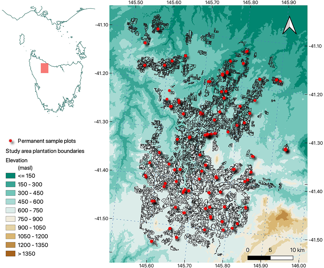
Figure 1. Study area plantation (black polygons), permanent sample plots (red star), and elevation (m.a.s.l.) (projection EPSG: 3577).

The dominant soil types in the area are Ferrosols, predominantly formed on basalt parent material, which are high in free iron oxides, contain a higher level of organic carbon (mean 6.5%), and are known for their desirable agricultural productivity (Cotching et al., 2009), despite being prone to deterioration through intensive management. Dermosols and Rudosols are also present in smaller areas across the plantations. This region is generally characterized as having good quality, deep and fertile soils, and with its temperate and wet climate, it is the most agriculturally productive in Tasmania.

A total of 161 plantation permanent sample plots (PSP) of 400 m² each were measured at regular intervals as part of the forest inventory. A total of 1,048 measurements cover aspects of tree growth (an average of six measurements per PSP rotation); primary measures being tree diameter at breast height (DBH), tree height (H), basal area (BA), stand volume (SV), and mean annual increment (MAI) were calculated based on mean H and DBH. The PSPs have between 5 and 10 measurements through the rotation of the plots (from establishment to harvesting), providing a robust basis for a time series of growth attributes.

2.2. 3-PG model

The 3-PG model was developed with the objective to be a practical tool for forest managers and researchers (Landsberg J. J. and Sands P. J., 2011). It combines simplified representations of biophysical processes with empirical relationships of growth and yield derived from field measurements. The default is a monthly timestep, although software extensions allow for daily timesteps to align with daily patterns of rainfall (Almeida and Sands, 2016). An overview of the core components of 3-PG is shown in Figure 2, adapted from Landsberg and Sands (2011). The full details of the model are outside the scope of this study; all the model components are well described in Landsberg and Waring (1997) and Landsberg J. J. and Sands P. J. (2011).

FIGURE 2

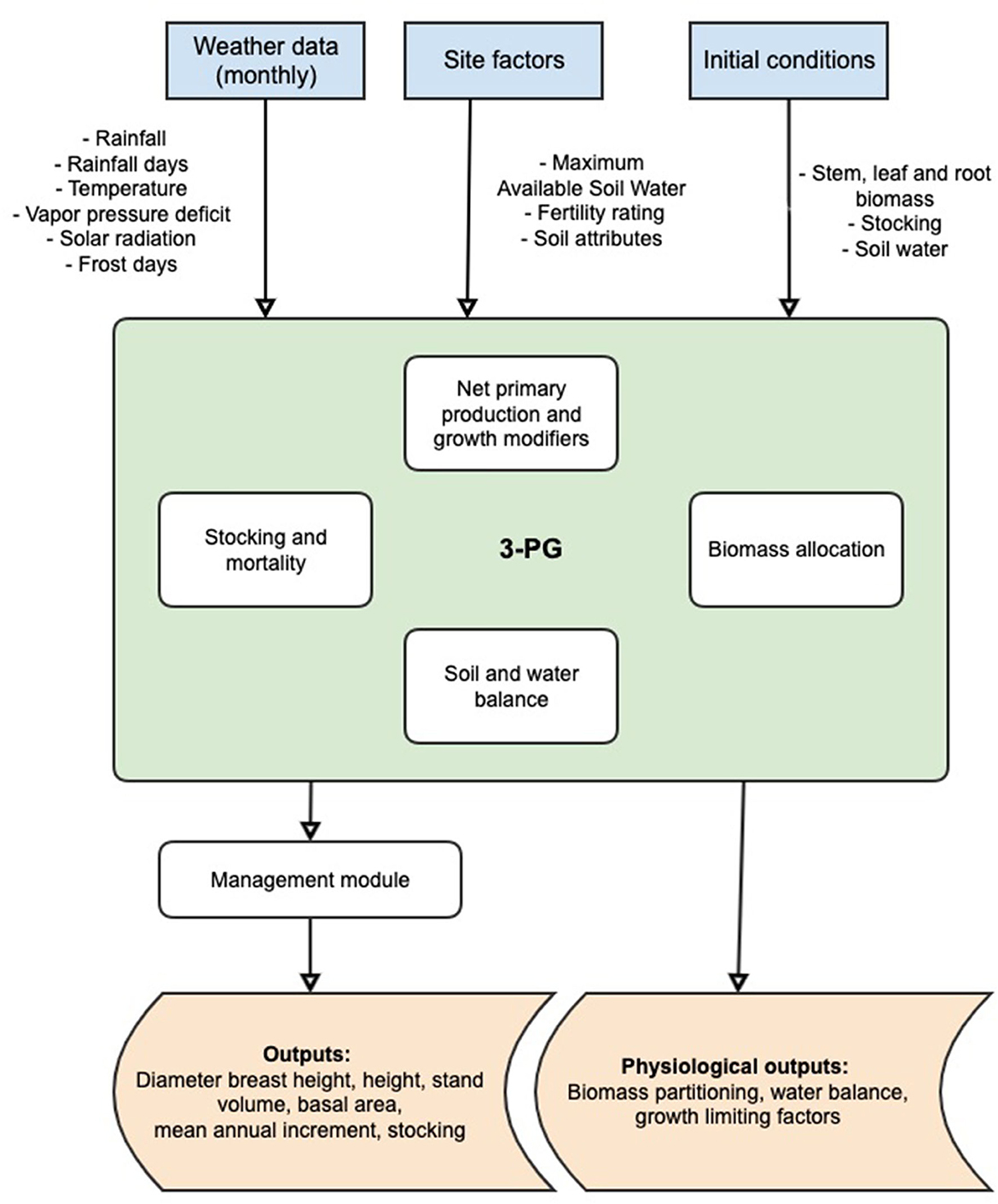
Figure 2. Simplified schematic representation of the 3-PG model (modified from Landsberg and Sands, 2011).

The 3-PG model has been successfully applied in many regions of the world (Gupta and Sharma, 2019) to various species, including different Eucalyptus plantations—E. globulus (Sands and Landsberg, 2002; Vega-Nieva et al., 2013; Carrasco et al., 2022), E. nitens (González-García et al., 2016), E. regnans (Feikema P. et al., 2010), E. grandis (Almeida et al., 2004; Stape et al., 2004b) and other plantations such as Pinus radiata (Feikema P. M. et al., 2010) and Pinus elliottii (Gonzalez-Benecke et al., 2014), and mixed species (Forrester and Tang, 2016). More recently, Forrester et al. (2021) demonstrated 3-PG performance when parameterised to major central European tree species.

The model can be applied at different scales, the most common application being plot scale, whereby the model represents individual plots of homogenous or mixed species, soil, and climate combinations (Gupta and Sharma, 2019). Spatial versions of the 3-PG model-−3-PGS—have been developed to capture and represent spatial variation of stand characteristics (Coops et al., 1998; Almeida et al., 2010). These versions are able to generate spatial outputs that provide additional insights for decision-makers (Tickle et al., 2001) under current and future climates (Almeida et al., 2009; Carrasco et al., 2022). This study uses both the plot and spatial scales of the 3-PG model: the plot scale for calibration and validation, and the spatial scale to expand the spatial coverage to provide predictions across all plantation areas, not just those with permanent sample plots.

2.2.1. Existing methods to determine soil fertility rating

There is no single agreed-upon method for estimating FR within the published literature; methods range from subjective site assessment to soil chemistry testing and incorporating combinations of soil and terrain characteristics (Dye et al., 2004; Stape et al., 2004b; Fontes et al., 2006; Paul et al., 2007; Xenakis et al., 2008; Almeida et al., 2010; Pérez-Cruzado et al., 2011; Vega-Nieva et al., 2013; Gonzalez-Benecke et al., 2014; González-García et al., 2016; Hung et al., 2016; Subedi and Fox, 2016; Carrasco et al., 2022). Other methods may incorporate a soil-nutrient sub-model that can capture the dynamics of the nutrient influence and exchange (Dewar, 2001). Some studies consider a gradual decay of FR values along the rotation length as the trees get older (Almeida et al., 2004). These are not covered directly here as we focus on methods that make direct use of data without major alteration of the model processes.

Published methods to determine the FR parameter for 3-PG generally use field-based measurement, expert knowledge of soil and/or the site, a data-driven method (including ML), calibration, or a combination of these. Table 1 summarizes some of the published examples of these methods.

TABLE 1

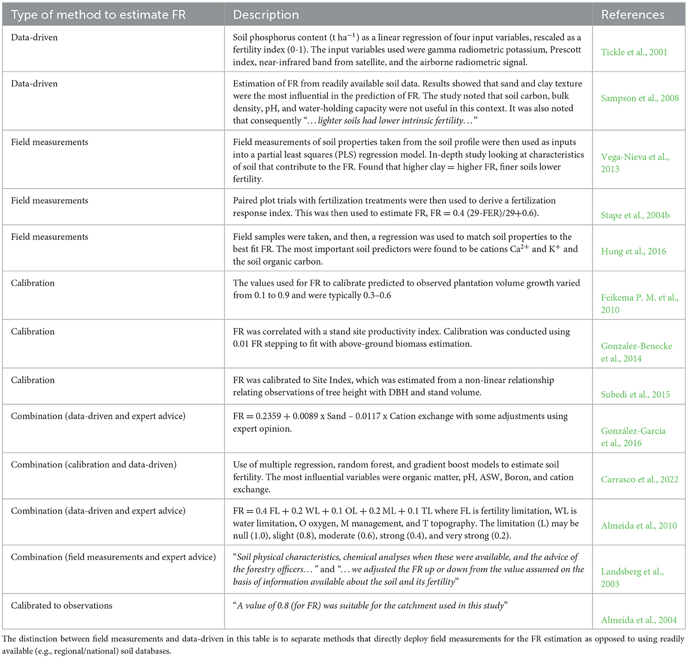
Table 1. Summary of published methods to estimate soil fertility rating (FR) in the 3-PG model.

The proposed method of applying machine learning provides an FR estimation technique that combines soil and terrain characteristics that may influence soil fertility and tree productivity. The method provides a reusable approach to test spatial variation and the performance of different machine learning models, while also providing transparency of the models using interpretable ML techniques.

2.3. Model input data

The input data required for the 3-PG model include details of soil attributes, climate, and site-specific attributes, such as stocking number (tree/ha) and initial planting biomass partitioning in leaves, stems, and roots (t/ha). The following sections provide detail of the inputs used.

2.3.1. Climate data

Monthly climate data of precipitation (mm), minimum and maximum temperature (°C), and solar radiation (MJ m⁻² day⁻¹) were obtained in gridded form from the SILO database (Jeffrey et al., 2001). Point time series at each plot location were extracted from the gridded data for use in the plot model. Additionally, the number of rain days and frost days in a month was derived as the count of the number of days with rainfall over 1 mm and daily minimum temperature below or equal to 0° C, respectively. Further details of the climate input data are available in the Supplementary material.

2.3.2. Soil, terrain, and terrain-adjusted climate data

Soil data were obtained from the Soil and Landscape Grid (Grundy et al., 2015; Kidd et al., 2015; Rossel et al., 2015) at a resolution of 3 arc-s, resulting in a grid of 876 columns and 962 rows, with each cell roughly 80 x 80 m. These grids are available for a range of textural and chemical soil attributes and at multiple depths, covering: 0–5, 5–15, 15–30, 30–60, 60–100, and 100–200 cm vertical sections. The soil texture data were used in both the 3-PG model and the ML model. Soil texture and soil depth were used to calculate the soil water holding capacity that influences the model water balance.

For the ML training, all six soil depth profiles were used separately to analyse which depth provided the best relationship to soil fertility rating, as shown in Figure 3 (stage 2).

FIGURE 3

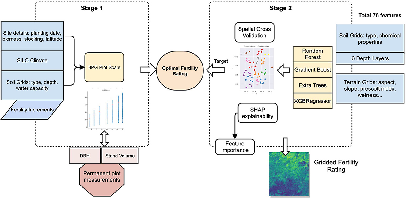
Figure 3. Data, 3-PG model, and ML processing workflow.

The terrain attribute data were obtained from published data that have been derived from 1" SRTM satellite data (Gallant and Austin, 2015), resulting in a grid size of 1,577 columns x 1,732 rows pixels. The attributes used are summarized in Table 2, with full reference to the data provided in the Supplementary material. There are also two terrain-adjusted climate variables and a climatic index used for ML models that are part of the Soil and Landscape Grid. These are not used in the 3-PG model.

TABLE 2

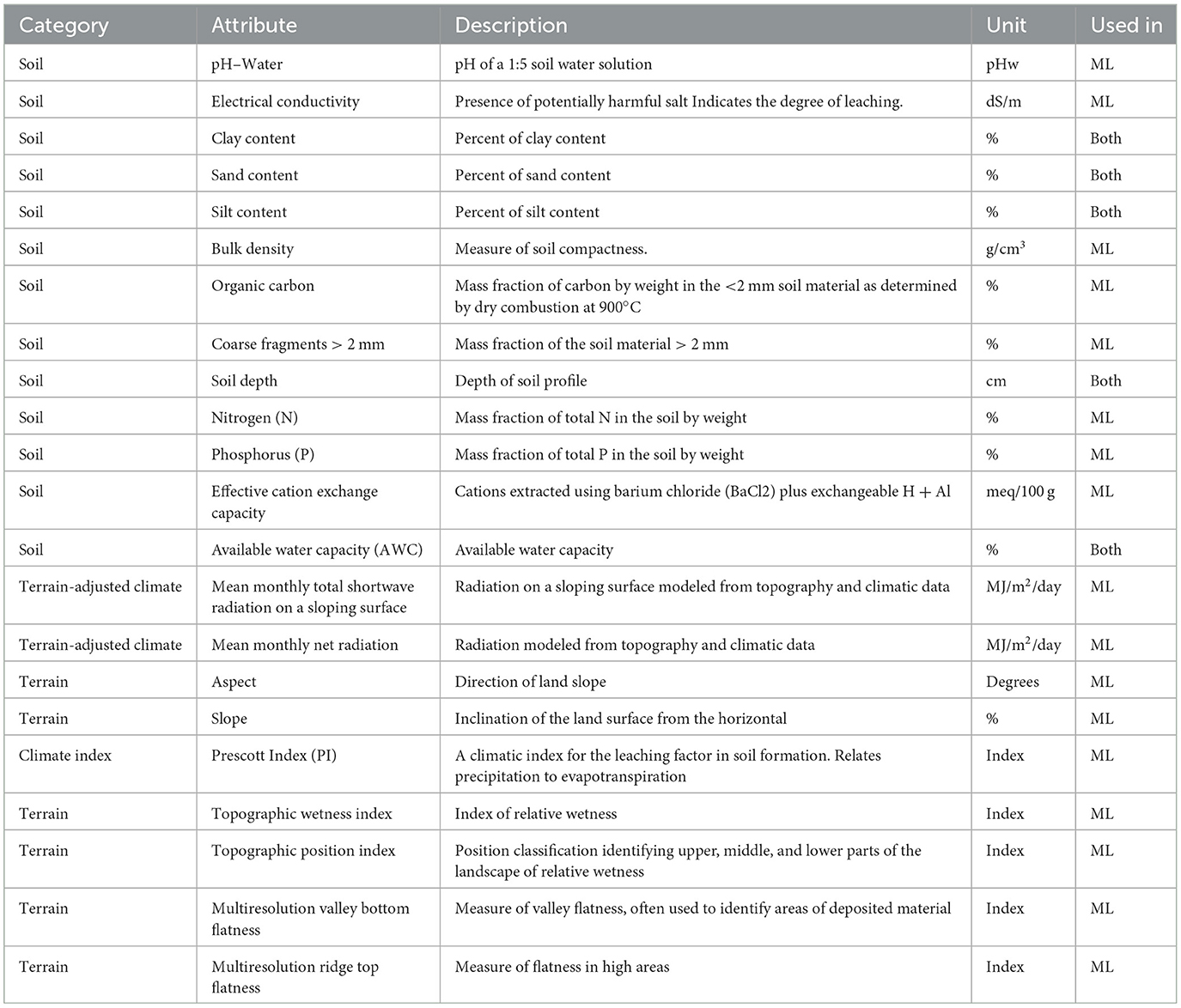
Table 2. Summary of soil, terrain, and terrain-adjusted attributes.

2.3.3. Model parameterisation

The 3-PG model requires a series of physiological and allometric parameter values related to the tree species. Many of the model input parameter values for E. nitens have been published in the literature from different tree physiology studies, particularly in Tasmania (Battaglia et al., 1996; White et al., 1996; Hunt and Beadle, 1998; Misra et al., 1998; Medhurst et al., 1999; Medhurst and Beadle, 2001, 2002; Moroni et al., 2003; Pinkard and Neilsen, 2003). Other studies have also been published applying 3-PG with parameter sets to E. nitens growing in other regions (Rodríguez et al., 2009; Pérez-Cruzado et al., 2011; González-García et al., 2016). The parameter values for E. nitens were reviewed and collated for the study area. This was done by selecting parameter sets from other E. nitens studies in Australia. The parameter descriptions, units, values, and sources are presented in the Supplementary material.

2.4. 3-PG and ML workflow

The process used in this study follows two stages: First, the setup and running of the 3-PG plot scale to determine the optimal FR for individual plots by matching the observed and predicted DBH and SV. These two outputs were selected as DBH is directly measured in forest inventory and SV is in general the most interest to forest managers and also derived from inventory measurements (Tickle et al., 2001). The second stage involved the training of ML models to predict FR from terrain and soil data. This two-stage process is shown in Figure 3.

An important characteristic of this workflow is that the 3-PG modeling to determine the optimal FR is done separately from the ML workflow. The 3-PG model incorporates influence from the climate, soils, water balance, plantation periods, and species information on plantation growth. The ML algorithms are then trained independently to determine the relationship between the soil and terrain attributes that explain the optimal FR values in each plot.

2.5. Stage 1−3-PG plot scale

This stage of the processing workflow involves running 3-PG at all plot sites using 0.01 increments of FR while fixing plantation details, climate, soils, and species parameter values. This method of using incremental FR is a simple approach to finding the optimal FR purely by fitting the model. It has been used in previous studies, as described in section Existing methods to determine soil fertility rating (calibration method), but it is not a recommended final method to estimate FR as it provides no relationship between the fertility and the soil or terrain. It becomes a tuning parameter only. It is used here to determine the target (or optimal FR) that can then be related to soil and terrain attributes.

The method then compares the DBH and SV with observed values to isolate the optimal FR values for every site. The steps are as follows:

1) Prepare model data inputs: climate, soil, site data, and species parameters.

2) Setup site definitions for each permanent plot location.

3) Run 3-PG plot scale model for FR at 0.01 increments between 0 and 1.

4) Compare 3-PG outputs (DBH and SV) to permanent plot location time series measurements.

5) Determine FR that minimizes the error between model and observed, for both DBH and SV. It does this by minimizing the average of the absolute per cent bias of the DBH and SV over all the FR model results from step 3, as shown in Formula 1.

\begin{array}{l} b i a s_{a v g} = \frac{(\frac{1}{n} \sum_{i = 1}^{n} | \frac{D B H_{o i} - D B H_{m i}}{D B H_{o i}} | \cdot 100 + \frac{1}{n} \sum_{i = 1}^{n} | \frac{S V_{o i} - S V_{m i}}{S V_{o i}} | \cdot 100)}{2} \end{array}

6) Where DBH_oi and DBH_mi are observed and modeled DBH at i^th measurement time, SV_oi and SV_mi are observed and modeled SV at i^th measurement time, and n is the number of measurements for the permanent sample plot.

2.6. Stage 2—machine learning prediction of FR

This stage uses only the FR values from the previous step as the target for the ML models, using terrain and soil as input features, with steps as follows:

1) At each permanent plot location, extract soil and terrain data. This generates 76 input features per plot location.

2) Train machine learning models using the combined data for all locations to predict FR from step 1.5 using soil and terrain data.

3) Compare machine learning model predictions.

4) Examine the internals of the predictions using interpretable ML to understand soil and terrain influence on predictions of fertility.

5) Select the best performing model using holdout R² and run predictions for each grid cell across the study area.

6) Using generated spatial fertility, run spatial 3-PG to generate gridded growth predictions.

2.6.1. Machine learning models

To predict the FR from soil and terrain data, four decision tree ensemble models were used: random forest regression tree (Ho, 1995) (RF), extra tree (or extremely randomized) regression tree (Geurts et al., 2006) (ET), gradient boost (Friedman, 2002) (GB), and XG boost (Chen and Guestrin, 2016) (XGB). This family of models was chosen for its desirable characteristics, specifically their ability to generalize to new data, moderate level of transparency and explanatory insight, ability to represent non-linear responses, and capture variable interactions, availability of implementation, and insensitivity to irrelevant predictors (Olden et al., 2008). Ensemble trees combine multiple estimators with the aim of improving predictions over single tree approaches, and the four ensemble models used can be grouped into two main families: RF and ET use averaging—also called bagging—of multiple estimators, whereas GB and XGB use boosting, which combine multiple weak learners to produce strong learners (Natekin and Knoll, 2013) by training additional estimators on the residuals of prior trees. More simply, bagging approaches train many independent decision trees and combine their predictions, while boosting sequentially trains trees where subsequent estimators learn based on the error of the previous trees. The differences in performance of these models are not absolute and depend largely on the area of application. Generally, the differences reside in how they optimize for either bias or variance in their predictions.

RF trees address the weakness of single decision trees by introducing a random selection of feature inputs to develop the splitting algorithm for each tree node (Breiman, 2001). ETs add additional randomness in the splitting rules by randomly selecting a cut point from the features, and they also use the whole sample when growing the tree rather than using a bootstrapped replica. The intention of the additional randomness in splitting seeks to reduce the variance in predictions; the change in the learning sampling aims at reducing bias (Geurts et al., 2006). ETs have potential efficiencies in computation times given the simplification of the splitting rule, whereas other ensembles require an optimisation to find an optimal cut point. For these two models, the training method used a randomized grid search to optimize the number of trees in the forest (number of estimators), the number of features used when splitting nodes (max features), the maximum depth, and the sample splitting size.

The two boosting tree models, GB and XGB, use the gradient boosting approach that sequentially trains trees that seek to improve predictions by learning from the errors of previous through minimizing a loss function. This process uses the slope—or gradient—of the loss function and trains subsequent trees to approximate this gradient to minimize the overall loss of the model. XGBs add regularization to GB models, which is a technique to reduce overfitting by penalizing higher weights for features, resulting in smaller and more spread-out weighting across features. XGBs also have additional improvements, including speed, early stopping, and inbuilt handling of missing values (Chen and Guestrin, 2016). Further details on each regression model are available in the cited references. The Scikit-learn (Pedregosa et al., 2011) Python package was used for all the ML model implementations, apart from the XGBoost Python implementation (Chen and Guestrin, 2016).

Other applications in environmental research have shown success in the use of tree models, for example, a study into ML to predict crop yields in Mexico noted that tree models performed better than ANNs (Gonzalez-Sanchez et al., 2014), while also highlighting the difficulty in model selection for environmental applications. A comparison of ML approaches for digital soil mapping (Heung et al., 2016) found RF and logistic model trees were desirable due to their speed and interpretability of results. RFs have also successfully been used in other spatial ML applications, such as tropical forest carbon mapping (Mascaro et al., 2014).

For this study, each model was trained and evaluated using the spatial cross-validation splits, using the group of six soil features (see Section Soil, terrain, and terrain-adjusted climate data) with the terrain data, with every split using a random grid search to optimize the ML algorithms hyperparameters. The hyperparameters for each model relate to the internal structuring of the trees when fitting. The hyperparameters are tuned by a random sampling approach that tests permutations of the parameter combinations and scores the results based on the scoring parameter. The commonly used correlation coefficient, R², was used as the scoring parameter, and root mean square error (RMSE) was also used in assessing both the ML and 3-PG model performance.

2.6.2. Spatial cross-validation

A spatial cross-validation approach was used to train and test the ML models. Cross-validation (CV) is a commonly employed technique to train ML models, especially when limited training data are available. Spatial CV is used in the presence of autocorrelation of data to avoid overoptimistic estimation of model performance (Meyer et al., 2019). It does this by using spatially aware splits of data, thus ensuring that training and testing data are spatially distinct. There is a current debate about the importance of spatially aware cross-validation methods (Wadoux et al., 2021) to assess map (model output) performance. A recent study tested the sensitivity to autocorrelation in a convolutional neural network's validation results, suggesting an overestimation of performance of up to 28% (Kattenborn et al., 2022).

The implementation of the spatial splitting used for the CV within this study was provided by the Digital Earth Australia toolkit (Krause et al., 2021). This includes different clustering algorithms that determine how clusters are grouped: K-means, Gaussian mixture, or hierarchical. The hierarchical method allows the specification of a Euclidean distance parameter to control the maximum distance within a group. Smaller numbers for this parameter result in clusters that are more spread out (to stay below the distance threshold); a larger distance parameter yields tighter clusters. Given this parameter affects the spatial grouping significantly and the sample size for this study, we tested the sensitivity of the ML models by training for iterations of this parameter ranging from 0.04 degrees to 0.13 at 0.01 degree increments. The count of clusters for the CV was set to 5 (5-fold), resulting in four training clusters and one for validation for each fold. This approach ensures training results are not overoptimistic, while additional resistance against overfitting.

An additional holdout set of 15% of the sites were used for validation, and not used in the spatial cross-validation, providing additional verification against overfitting. These holdout sites were also selected using a spatial separation split approach, where 15% of sites are in an area unseen by any of the ML models. 15% and K-5 splitting were chosen due to the relatively small sample size (161 plots) to avoid reducing the available sites for cross-validation too significantly.

The trained models were then filtered to select the highest mean R² model achieved in the cross-validation.

2.6.3. Interpretable machine learning

The game theory-based method (Štrumbelj and Kononenko, 2014) to interpretable machine learning was used, as implemented in the SHAP (SHapley Additive exPlanations) library (Lundberg and Lee, 2017). This method quantifies each input feature's importance in making predictions. It does this by perturbing the model's input features to generate an estimate of its contribution to individual predictions. This provides normalized values that can be inspected and compared for different individual (local)—and overall (global)—contribution to predictions.

Within stage 2 of the processing workflow, force plots (Lundberg et al., 2018) were used to explore the influence of the soil and terrain variables on the prediction of site FR. This provides the magnitude and direction of a specific input's contribution, allowing examination of the consistency of predictions and the relation to specific sites.

3. Results

3.1. 3-PG plot scale calibration of FR

The distribution of FR results from stage 1 is shown in Figure 4 by latitude (a), longitude (b), and overall probability density (c). Plot (a) shows some indication of a trend of lower FR in the southern plots. This trend is shown further in the spatial outputs from the ML models in Results section.

FIGURE 4

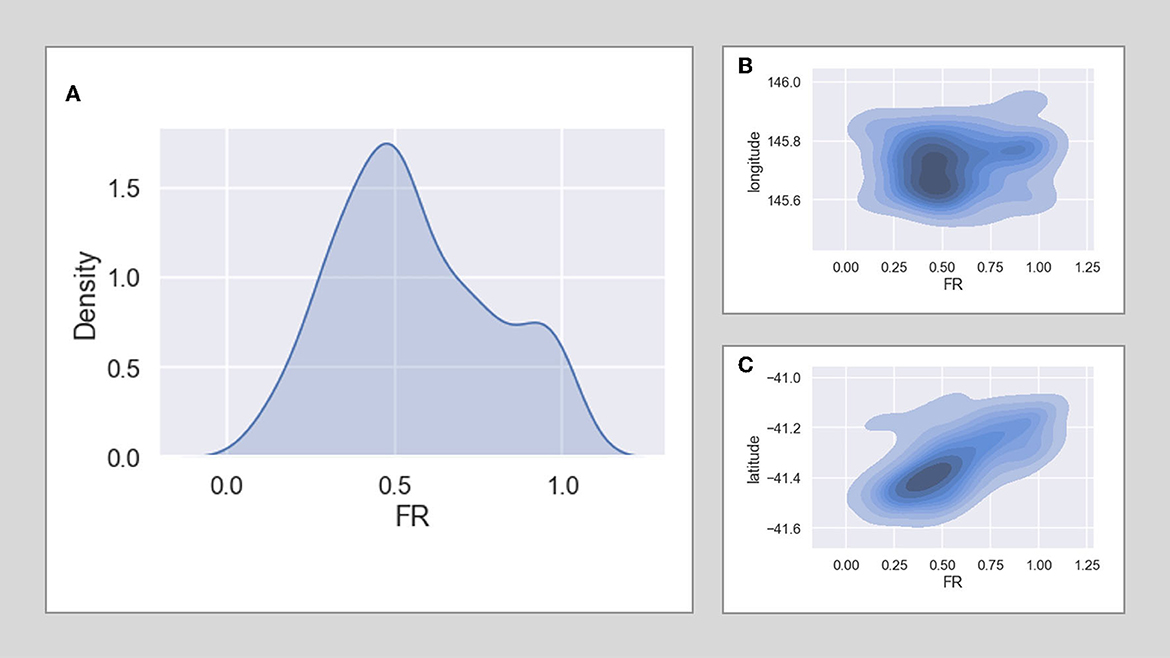
Figure 4. Probability density of FR of all plots density (A) by longitude (B) and latitude (C).

3.2. ML training and cross-validation results

The cross-validation is executed for combinations of the ML model, soil feature groups and Euclidean distance parameters, with a random grid search for the hyperparameters of each model. The best performing hyperparameter set is selected based on its mean cross-validation score across each fold.

Figure 5 shows the results for predictions in the training and holdout data grouped by soil depth when selecting the best performing distance parameter. The best performing depth profile for training was 15 cm (R² = 0.49) and the holdout was 100 cm (R² = 0.73). The holdout results (mean R² = 0.66) show better performance than the cross-validation fold results (mean R²= 0.44), providing some evidence that the model can spatially generalize to unseen data. The best performing model in training was ET (R² = 0.72) and in holdout was RF (R² = 0.78).

FIGURE 5

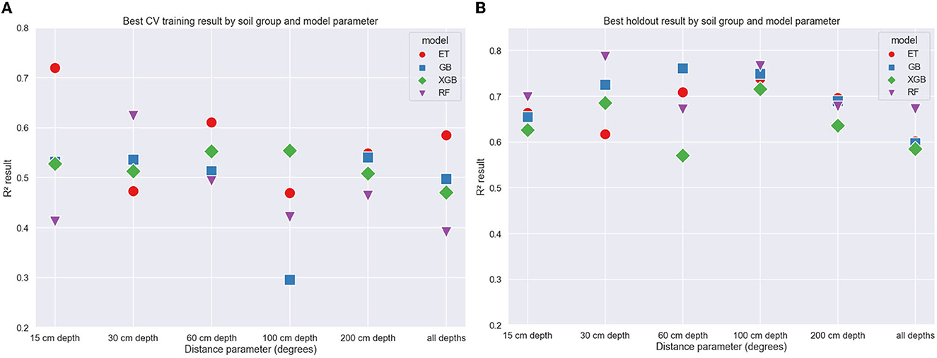
Figure 5. Coefficient of correlation (R²) values vs. soil depth group for training (A) and holdout (B) data grouped by model.

The variation of the maximum distance parameter provides an estimation of how sensitive the cross-validation results are to the spatial grouping structure. Results grouped by the maximum Euclidean distance parameter are shown in Figure 6. The correlation variance appears to increase as the distance parameter increases and is more pronounced in the training data. The higher distance parameter clusters will result in points closer together, so the validation group will cover a smaller area and will likely have less FR variation. The RF model shows the best result when considering the holdout data, and the ET models show better results for the mean CV training.

FIGURE 6

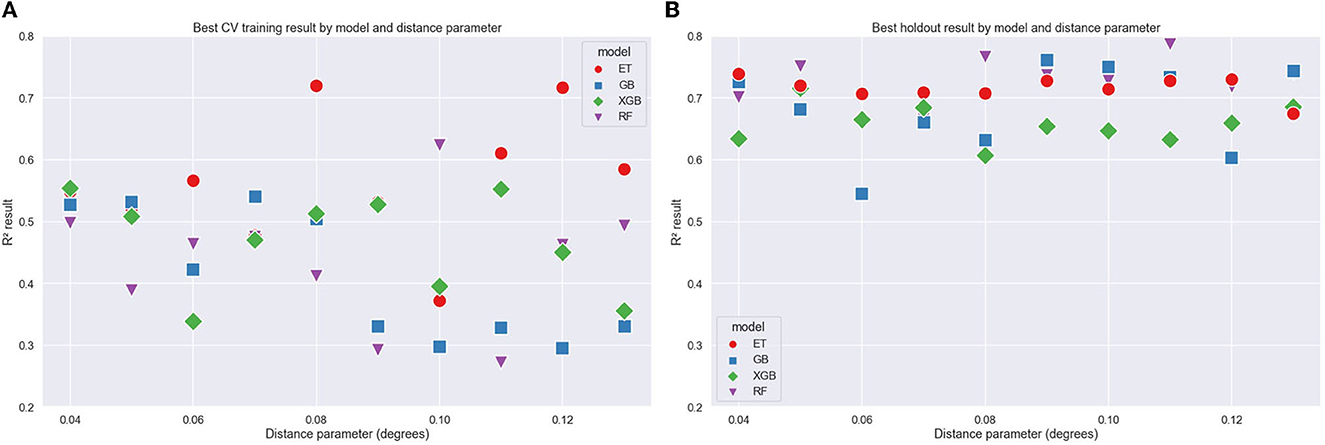
Figure 6. Coefficient of correlation (R²) values vs. Euclidean distance parameter for training (A) and holdout (B) data grouped by ML models.

When considering the average of the training and holdout results, the ET model had the top five best ranking models, with mean R² across training and holdout of 0.64, 0.63, 0.63, 0.61, and 0.61. The best of each of the four models using average R² was ET = 0.64, RF = 0.61, GB = 0.59, and XGB = 0.54. To check the full set of predictions, the best performing model from the cross-validation results and the best performing model when comparing to the holdout data were run against the training and holdout data to compare predicted with actual values. Both show a good correlation between predicted and actual values. Some models showed clear signs of overfitting with training values fitting a straight line; the use of the holdout data set assisted in the identification of these models that could be excluded.

The computational requirements for training the models were not high. The total training time was in the range of 2–3 h using an 8-core i9 machine with 64 GB RAM. Within this time, the ML models were converging on optimal solutions, and thus, further training was not necessary.

3.3. Feature importance results

The top-performing models were selected by filtering models with a CV R² > 0.3 and selecting the best holdout R² score for each ML model type. The SHAP values were computed to understand the features that have the strongest influence when making predictions. Table 3 shows the top five features of the best performing model for the four models. This table summarizes the more detailed SHAP value plots in Figure 7.

TABLE 3

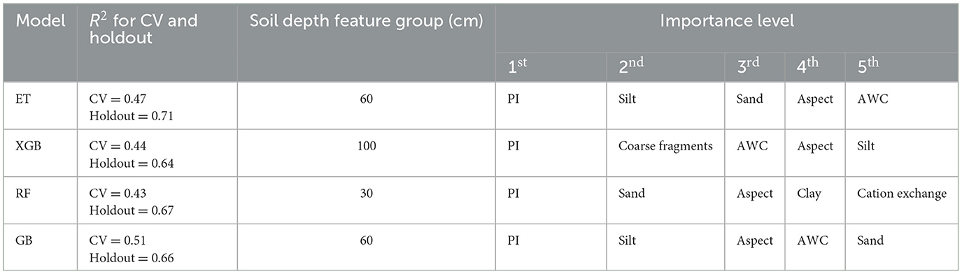
Table 3. Most important features for the top six models (selected by best performing model against holdout data).

FIGURE 7

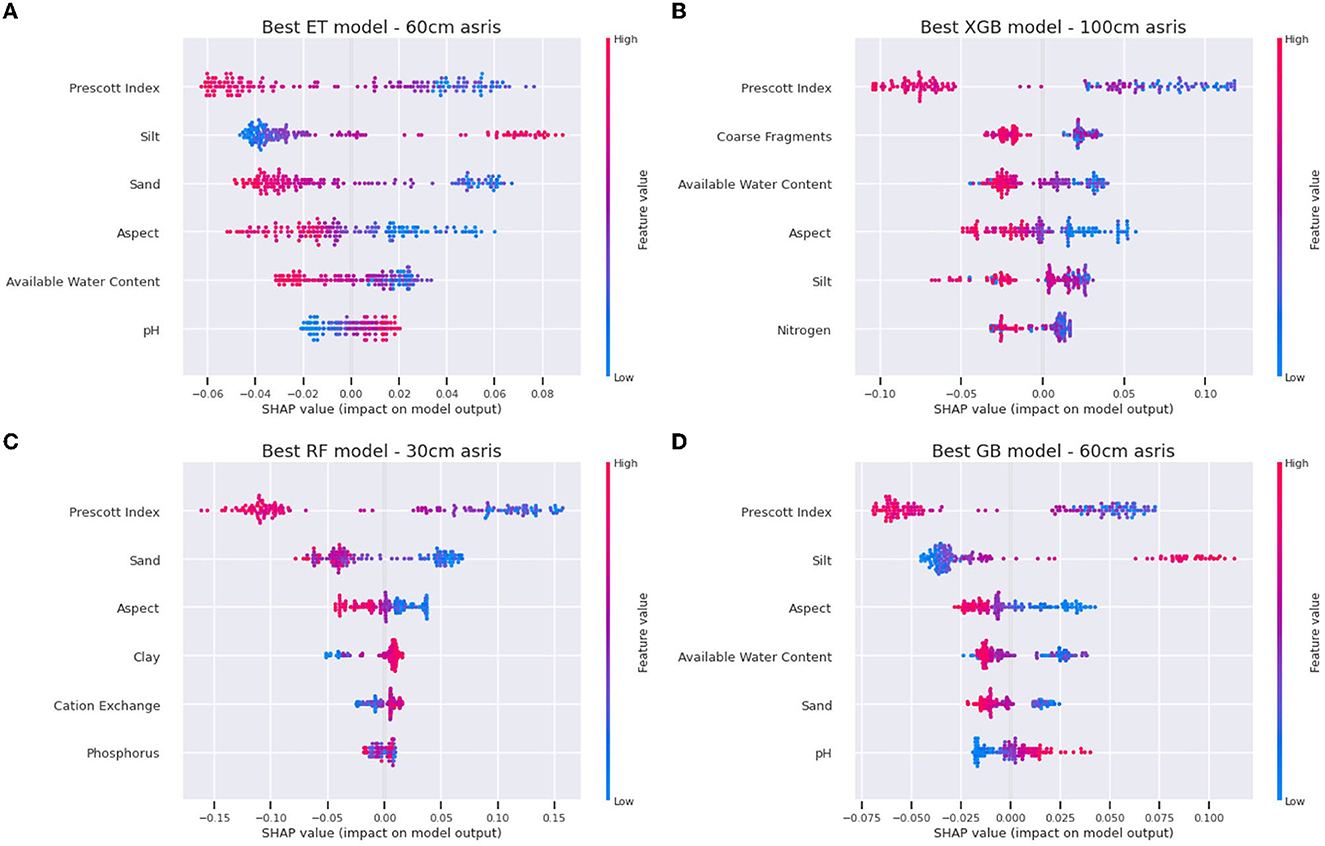
Figure 7. SHAP values for top six features for the best performing model in each model type—(A) Extra-Tree regressor (ET), (B) XGB (eXtreme Gradient Boost), (C) Random Forest (RF), and (D) Gradient Boost (GB).

The Prescott Index (PI), a measure of soil–water balance, is consistently used by all models and has the highest influence on predictions. Site aspect, available water content, and textural soil components (sand and clay content) are all regularly used in predictions. The next section provides results on how these features influence the FR predictions.

3.3.1. Feature influences on predictions

The SHAP values were generated to produce influence plots for the top four models, shown in Figure 7. This shows the influence of the top 6 features in the predictions for all locations, showing the top-performing model for each of the four ML models. There appears to be consistency across the ML models in the way the input features have influenced the FR predictions. For example, in all four of the models shown in Figure 7, a high PI value (pink) indicates lower FR (lower SHAP value). And for the soil sand content, the ET, RF, and GB models show that a higher sand content also results in lower FR (lower SHAP value).

The aspect terrain attribute is a direction vector with units of degrees and thus needs appropriate interpretation in terms of its values and influence. SHAP dependence plots show the relationship of feature values with the predictions, providing more details of a feature's influence. Figure 8 shows a dependence plot for aspect, with the 0–180 boxes indicating the values of aspect that are positively affecting FR, which corresponds to a north-east (NE) aspect, as opposed to the south-west (SW) (180–360 degree) aspect sites that show a decrease in FR. This follows intuitively that NE sites have more exposure to solar radiation than the SW-facing sites and are less exposed to wind predominance that can cause damage to the leaves. The influence of aspect (and slope) on both soil processes and plant growth is well known and documented elsewhere (Reid, 1973; Holland and Steyn, 1975; Beaudette and O'Geen, 2009).

FIGURE 8

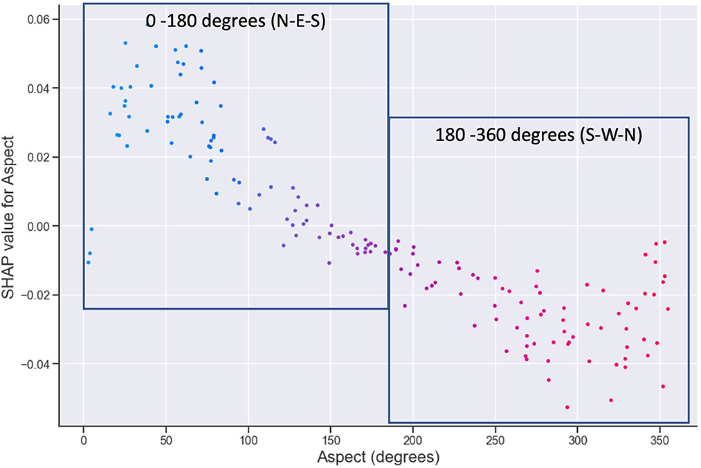
Figure 8. Influence of terrain aspect on prediction of FR.

3.3.2. Assessing site-level (local) FR predictions

SHAP decision plots were used to describe individual predictions (sites in this instance). Figure 9 shows decision plots for four test sites. These sites were selected as exemplar high- and low-productivity sites, to check for comparison against the predictions of the model, and to assess how these relate to both the 3-PG model plantation growth and the FR predictions. The test site details are shown in Table 4, and the corresponding decision plots are shown in Figure 9. The decision plot shows how the prediction for each site is being influenced by the soil and terrain attributes. The attributes on the Y axis are sorted in descending order of influence, showing the four most influential properties being the PI, sand, clay, aspect, and cation exchange. These are consistent with the overall influence plots for all sites in Figure 7, though the relative importance is different, and silt does not show as being highly influential for these sites.

FIGURE 9

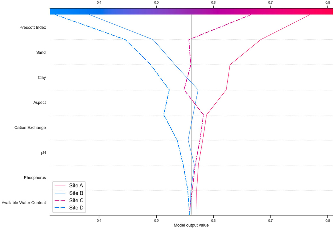
Figure 9. SHAP decision plot showing predictions for four specific sites for the best fit RF model.

TABLE 4

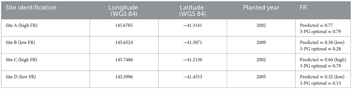
Table 4. Details of four test sites to compare predictions.

3.4. Applying predicted FR with 3-PG

Using the best scoring ET model, we ran the predictions of FRs across every grid cell for the study area to produce a spatial map (grid) of FR. Figure 10 shows the output of this process, with the scale going from low FR (dark red, 0) to high FR (dark blue, 1). FR values and respective per cent areas are shown in the histogram.

FIGURE 10

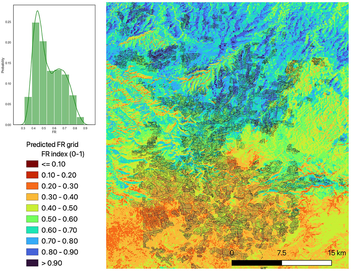
Figure 10. ET model-derived fertility rating at 1 arc-s (~30 m) resolution covering study area. Shadow areas show plantation boundaries. Histogram shows probability density for each category across the whole area.

The predicted FR was used to parameterise the 3-PG model and run in both plot and spatial scales. The generated FR layer provides the spatial estimation of fertility rating for the whole plantation area, which can then be used to model to predict potential productivity across the region, showing the spatial distribution of expected growth under current or future climate scenarios. Results for potential productivity as stand volume for the area planted in 2006 and grown for 12 years are shown in Figure 11.

FIGURE 11

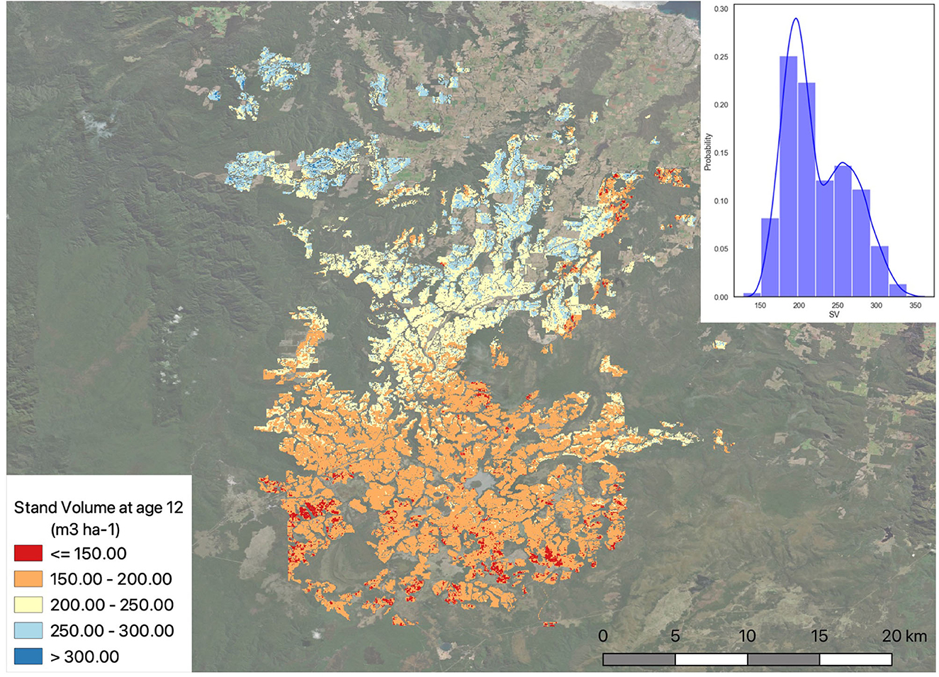
Figure 11. Potential productivity for the study as stand volume (m³ ha⁻¹) considering all areas planted in 09/2006 and grown for 12 years. Histogram shows probability (%) density for the SV ranges.

A comparison of the 3-PG results using the ML-derived FR and using the optimal FR across all plots showed strong agreement. R² differed by only 0.01 for DBH (0.97 vs. 0.98), SV (0.96 and 0.97) and H (0.96 and 0.97), and 0.02 for BA (0.95 and 0.97) and 0.03 for MAI (0.93 vs. 0.96) for the ML-derived model and the model with optimal FR values. The optimal FR model uses the best fit method described in the method section—i.e., it is directly calibrated to fit the observations. While optimal, the fitting provides no explanation in terms of its contribution to the growth and how this relates to any soil or terrain attributes.

4. Discussion

This study has demonstrated the utility of a machine learning-based method to estimate FR for use within the 3-PG forest growth model to improve the accuracy of the model predictions. The contributions of this approach are 2-fold. First, it provides a reusable and interpretable method to estimate the 3-PG FR parameter from spatial data of soil and terrain attributes. This can be used to parameterise both plot and spatial scales of the 3-PG model. Second, it allows the generation of spatial FR and estimates of the influencing variables that can be used to inform forest management decisions, such as plantation and rotation cycles. The generated spatial data can assist in identifying areas of potential low and high productivity and providing valuable information for forest planning and wood supply management. Additionally, the influence of soils and terrain on fertility can be inspected for each site using the SHAP method described. This allows detailed spatial analysis when assessing variability in productivity.

The four ML regression models spatially estimated FR across the study area using inputs from spatial soil and terrain data. The subsequent 3-PG results show very accurate predictions when comparing model outputs to stands with different ages and periods and different site-related variables. That inference power of the ML-derived FR rating as an input to 3-PG is demonstrated by its performance in capturing growth dynamics across subsequent rotations and under different climate periods, as opposed to just fitting a singular growth variable.

When compared to a simple calibration, or fitting, of the FR, the ML method can generate spatial predictions using the terrain and soil attributes, resulting in high-resolution spatial grids of soil fertility. These can then be used in the spatial version of 3-PG and as indicators of plantation productivity.

4.1. Influence of soil and terrain features

The results of ML models show that the most influential features were PI, textural components (mainly sand and silt), and aspect. There was low influence observed from the N or P soil layer, and this has also been noted in other studies for E. globulus and P. radiata in Chile (Carrasco et al., 2022). The PI appears to be the dominant explanatory variable, and while PI describes the soil water balance, it also relates to the soil's ability to hold nutrients. For example, higher PI indicates greater leaching of soils related to the ratio between precipitation and evapotranspiration and has been shown to relate to soil pH in Australia (de Caritat et al., 2011), which in turn may affect nutrient availability (Neina, 2019). The N and P contents of the soil may change due to management practices, for example, through soil cultivation and application of N and/or P on trees. However, these short-term changes are not reflected in the static soil grids; while a surrogate variable such as PI is more likely to capture short-term soil-nutrient dynamics and therefore be an important explanatory variable for the FR.

The influence of the aspect feature may be identifying sites that have improved solar radiation exposure, as shown by the increased FR for north-east-facing sites. Alternatively, it may be the influence of wind exposure, with the predominant west winds affecting growth and/or soil composition, or a combination of solar radiation and wind effects. The SILO radiation values used for 3-PG are not adjusted for aspect (https://www.longpaddock.qld.gov.au/silo/faq/) and 3-PG does not explicitly capture site aspect, though it does model light interception from the canopy. Terrain-adjusted mean-monthly net radiation was used as an input feature (see Soil, terrain, and terrain-adjusted climate data), which adjusts for aspect and slope attributes (among others), but this was not identified as an influential attribute in the top-performing models.

Given the textural components are interrelated, specifically sand, silt, and clay content, water holding capacity, and coarse fragments, the models are likely to perform similarly when subsets of these attributes are used. The sensitivity to subsets of the textural attributes was not tested but warrants further investigation. Noting that the SHAP feature analysis contains internal handling of correlated features by perturbing combinations of different features and has been proposed as a feature selection processor (Marcílio and Eler, 2020).

There are different methods to ML model interpretation, including Local Interpretable Model-agnostic Explanations (LIME), permutation feature importance (PFI), and SHAP (as used in this study). These approaches vary in their method and will thus provide different results. The SHAP was chosen given its flexibility and range of available plots for analysis. Studies have shown that PFI is less useful in the presence of correlated input features (Kaneko, 2022). PFI was calculated for many of the trained models and noted that the top five identified features were often similar, with slight variations in the feature order. While these helped to inform how the models are forming predictions, further study is required to relate these features through the FR to its effects on the 3-PG model.

There was not a clear pattern in the prediction performance across the six groups of soil depths tested. These layers contain a level of internal correlation (see Supplementary material for details), and the differences may not be significant enough to influence the outputs from the ML models. Depending on the available data, the soil depth profiles are harmonized and derived (Rossel et al., 2015) and thus may not contain sufficient variation, or the signal may be weaker than other soil attributes. The chemical attributes of the soil grid have also shown higher uncertainties and high spatial variability than the textural attributes (Kidd et al., 2015).

4.2. ML model performance

The four ML models that were tested did not show large differences in their performance; though when considering the average R² across training and validation, the ET model had the top five best ranking models. The ET model is probably benefitting from the additional level of randomness where the splitting rule for the tree structure uses a random selection as opposed to the RF model which selects the best split each time. The holdout results were generally higher, which suggests the models can generalize to unseen data. However, this needs to be considered in the context of the random test-train split from this small-sized data set; the spatially split cross-validation provides a more robust metric of performance. The use of the spatial splitting for both cross-validation and holdout testing provided a useful approach to identifying models that were overfitting on the training data, especially for a small sample size as in this study. The spatial splitting helps to avoid leakage of the training data into the validation sets where there may be proximal sites in both sets.

There was consistency in the most important features being selected, with some variations that would be expected given some internal correlation of input features. The issue of equifinality arises, where multiple models with different parameterisations can produce equal accuracy, as has been noted with ML applied to hydrology (Schmidt et al., 2020).

4.3. Relationship to other studies

As described earlier, there are existing methods to estimate the FR parameter of 3-PG. Some of these have also used multiple regression and decision trees to provide estimates (Tickle et al., 2001; Hung et al., 2016; Carrasco et al., 2022). However, to our knowledge there are no published methods that focus on the FR estimation using ML that include spatial cross-validation, the use of SHAP techniques for variable interpretation, and incorporation of the range of spatial soil and terrain data described in this study. The method used in this study could be described as a combination of data driven with calibration when relating to other FR estimation methods (Table 1). These existing FR estimation methods were adapted based on the context of the application of 3-PG, specifically in terms of data availability, access to field data, and any potential input from soil experts. Given the increasing availability of gridded soil and terrain data, the method described can be reproduced with access to appropriate levels of soil and terrain data. This is particularly the case when field-based measurements are not a viable option to estimate FR.

This study only used tree-based regression method; there are many more ML regression methods that may be utilized, such as artificial neural networks (ANNs), support vector machines, and k-nearest neighbor learners, among others. As described in Method section, this study selected the method by balancing the requirements of the study. Given the sample size, compatibility with interpretable machine learning libraries, and reasonable performance that was obtained through the four tree-based models, it was not deemed necessary to include other ML models for this study. This could, however, be explored in the future study.

4.4. Assumptions and limitations of this study

The spatial cross-validation method used in this study accounts for a level of autocorrelation in the spatial data. However, due to the study area size, the effects of spatial variability are likely to change at different (i.e., larger/global) scales. Therefore, this method requires testing across different spatial scales. Noting that as the spatial scale changes, the overall variables that influence growth are also likely to change due to differences in physical processes at these scales. The challenges associated with local vs. global map accuracy derived from ML models are discussed by Meyer and Pebesma (2022). The authors caution on the use of global-level indicators of map accuracy and derivations of these models. This study claims no specific relevance of these results at a global scale; however, the method here is reusable for studies and applications of 3-PG or other models requiring derived soil properties for a study of the same scale. The use of holdout data in addition to the CV training data provides an additional round of validation of the results. However, the small sample size and randomness in sample selection for holdout comparisons can skew results, both negatively and positively, and must be evaluated alongside the full CV results.

The described method does not currently account for any temporal variation in soil fertility. This is clearly a simplification, but one that is necessary with the availability of data at this scale. Certain soil attributes will be more static through time than others, such as the textural components, whereas the chemical attributes, such as N, P, and organic carbon, would vary and thus influence soil fertility. Noting that the most important attributes within this study related to textural and terrain attributes.

The 3-PG model was tested against the five main growth outputs, but the soil moisture state of the model was not compared to any direct measurements of soil moisture due to none being available. The model was informally tested against a national water balance model and showed a good correlation. It would be desirable to test the soil moisture balance more intensively in future. Additionally, it would be desirable to further test the spatial predictions of FR on plantation areas outside this study area. This would provide further validation of the ability of the ML models to generalize.

The applied method combined with the 3-PG model produced accurate spatial predictions of the main outputs of interest for forest management allowing to indicate the factors that influence forest growth.

5. Conclusion

This study has described a machine learning method to estimate site soil fertility that has the benefit of exposing the core explanatory variables for predictions and can be applied to point-based or spatial versions of the 3-PG model. The derived soil fertility grid can be used directly in spatial 3-PG models and is also valuable as a plantation management dataset to show spatial variability of productivity in unknown areas. Comparisons across the four regression tree models show a level of consistency in the selection of soil and terrain attributes as explanatory variables for the regression models. While causation cannot necessarily be presumed from these explanatory variables, the predicted FR can be used with the 3-PG model to accurately simulate growth and provide a transparent basis for the derivation of the soil fertility parameter, leading to improved accuracy to support plantation management decisions.

Data availability statement

The original contributions presented in the study are included in the article/Supplementary material, further inquiries can be directed to the corresponding author.

Author contributions

AA, EK, and PT conceptualized project. AA, PT, EK, and RA acquired all data, contributed relevant knowledge to the project and result interpretation, and contributed to the paper writing. PT and AA implemented the 3-PG spatial models and implemented 3-PG plot scale. PT implemented ML workflows. All authors contributed to the article and approved the submitted version.

Acknowledgments

The authors would like to thank the contributions from the Forico team for interactions, field visits, and providing data and to Matthew Webb and Darren Kidd from the Department of Natural Resources and Environment (DPIPWE) for their contributions to soil and climate data for the region. The authors would like to thank Stephen B. Stewart (CSIRO Environment) and Daniel K. Smith (CSIRO Data61) for their detailed reviews and excellent suggestions on the study. The authors would also like to thank the two reviewers for their very constructive reviews and suggestions.

Conflict of interest

EK and RA were employed by Forico Pty Ltd.

The remaining authors declare that the research was conducted in the absence of any commercial or financial relationships that could be construed as a potential conflict of interest.

Publisher's note

All claims expressed in this article are solely those of the authors and do not necessarily represent those of their affiliated organizations, or those of the publisher, the editors and the reviewers. Any product that may be evaluated in this article, or claim that may be made by its manufacturer, is not guaranteed or endorsed by the publisher.

Supplementary material

The Supplementary Material for this article can be found online at: https://www.frontiersin.org/articles/10.3389/ffgc.2023.1181049/full#supplementary-material

References

Almeida, A. C. (2003). Application of a process-based model for predicting and explaining growth in Eucalyptus plantations (PhD Thesis). The Australian National University, Canberra, Australia. p. 232.

Google Scholar

Almeida, A. C. (2018). “Forest growth modelling for decision making: Practical applications and perspectives,” in New Frontiers in Forecasting Forests (Stellenbosch), 60–62. Available online at: http://hdl.handle.net/102.100.100/143403?index=1

PubMed Abstract | Google Scholar

Almeida, A. C., Landsberg, J. J., and Sands, P. J. (2004). Parameterisation of 3-PG model for fast-growing Eucalyptus grandis plantations. For. Ecol. Manag. 193, 179–195. doi: 10.1016/j.foreco.2004.01.029