 Subhash R. Lele
- Department of Mathematical and Statistical Sciences, University of Alberta, Edmonton, AB, Canada
An inferential statement is any statement about the parameters, form of the underlying process or future outcomes. An inferential statement, that provides an approximation to the truth, becomes “statistical” only when there is a measure of uncertainty associated with it. The uncertainty of an inferential statement is generally quantified in terms of probability of the strength of approximation to the truth. This is what we term “inferential uncertainty.” Answer to this question has significant implications in statistical decision making where inferential uncertainty is combined with loss functions for predicted outcomes to compute the risk associated with the decision. The Classical and the Evidential paradigms use aleatory (frequency based) probability for quantifying uncertainty whereas the Bayesian approach utilizes epistemic (belief based) probability. To compute aleatory uncertainty, one needs to answer the question: which experiment is being repeated, hypothetically or otherwise? whereas computing epistemic uncertainty requires: What is the prior belief? Deciding which type of uncertainty is appropriate for scientific inference has been a contentious issue and without proper resolution because it has been commonly formulated in terms of statements about parameters, that are statistical constructs, not observables. Common to these approaches is the desire to understand the data generating mechanism. Whether one follows the Frequentist or the Bayesian approach inferential statements concerning prediction are aleatory in nature and are practically ascertainable. We consider the desirable characteristics for quantification of uncertainty as: (1) Parameterization and data transformation invariance, (2) correct predictive coverage, (3) uncertainty that depends only on the data at hand and the hypothesized data generating mechanism, and (4) diagnostics for model misspecification and guidance for correction. We examine the Classical, Bayesian and Evidential approaches in the light of these characteristics. Unfortunately, none of these inferential approaches possesses all of our desiderata although the Evidential approach seems to come closest. Choosing an inferential approach, thus, involves choosing between either specifying the hypothetical experiment that will be repeated or equivalently a sampling distribution of the estimator or a prior distribution on the model space or an evidence function.
1. Introduction
It is indisputable that statistical reasoning has become an essential component of modern scientific thinking (Taper and Ponciano, 2016). However, discussions on the philosophical foundations of statistical methods are often regarded as esoteric and of little practical importance to the scientific practitioners (e.g., Clark, 2005). It is commonly claimed that pragmatic scientists somehow know which method is appropriate for their own problem and they do not need to worry about the differences in the philosophies of statistics that underlie such methods. That such differences are too subtle to be of any practical relevance (e.g., Kery and Royle, 2016). One possible reason scientists feel this way is because they often make decisions solely on the basis of the estimated effect size while paying only a lip service to the magnitude and nature of the associated uncertainty, in spite of the repeated protestations by the statisticians that “effect size estimate without the associated uncertainty” is useless for decision making. Understanding the meaning and the quantification of uncertainty is a major hurdle, both in practical applications of statistics and in understanding the arguments for and against different paradigms in statistics.
Why is uncertainty quantification a critical endeavor for science and scientific decisions? Decisions are ultimately based on the predictions of the future outcomes of a statistical experiment. These predictions are uncertain and hence we need to quantify their uncertainty. Prediction uncertainty has several components. First component is the process variation. It exists even if all the parameters of the model are known. This variation can be reduced to some extent by appropriate use of covariates and auxiliary information in the process modeling. Second component is the estimation error. This occurs because parameters in the process model are generally unknown and not directly observable. These parameters need to be estimated using the observed data. Different methods of estimation lead to different estimation errors. Both these components assume that the form of the model used for prediction correctly represents the true underlying process. The third component to prediction uncertainty is the uncertainty about the form of the process model. This uncertainty can be controlled to some extent by appropriate model selection and model diagnostics. Prediction uncertainty is a combination of these three components. Given the prediction uncertainty, we can combine it with the loss function that quantifies the consequences of different decisions that are based on the uncertain predictions. The combination of the loss function and the three types of uncertainties leads to the quantification of risk. A rational decision maker is presumed to choose a course that minimizes the risk. Thus, if one wants to make rational decisions, one needs a verifiable quantification of the uncertainty in prediction. In this paper, we discuss the quantification of the prediction uncertainty when there is no model form uncertainty. Dennis et al. (2019) discuss the effect of model mis-specification on the quantification of uncertainty.
The goal of this paper is to discuss various ways statisticians quantify uncertainty in statistical inferential statements about the parameters of the model and the observables. Here observables refer to both observed data and future data that are potentially observable. Parameters of the model, although statistical constructs and not always useful for prediction in specific circumstances, are important for developing scientific understanding (e.g., Jerde et al., 2019). However, uncertainty statements about the parameter estimates are difficult to directly verify in practice. On the other hand, statements about the observables are aleatory or frequentist in nature and hence are directly ascertainable in practice. Predictive accuracy has been at the center of much of the development in the statistical learning literature (e.g., Hastie et al., 2009) and has also been suggested as the appropriate approach to statistical thinking (Billheimer, 2019). We emphasize, however, that it is not sufficient to compare predictive abilities of different procedures. Ability to diagnose and pinpoint errors in modeling and being able to learn from errors is an essential component when comparing the desirability of various inferential procedures (e.g., Dennis, 1996; Lele and Dennis, 2009).
Although many of the discussions in the literature often concentrate on estimation and testing of the parameters of the model, the scope of statistical inference is wider than that. For example, scientists want to be able to forecast future outcomes under different “what if” scenarios or they may be interested in studying derived quantities, such as probability of extinction or time to extinction of a species. Model choice, estimation and prediction are three important components of any scientific enquiry. In the next section, we discuss desiderata for uncertainty quantification in the context of this general scope. In section 3, we will discuss the basics of the Classical paradigm to quantify uncertainty. We emphasize the difference between pre-data and post-data measures of uncertainty and difficulties faced by the Classical approach. This will lead us to the discussion of conditional inference, relevant subsets and ancillary statistics. We discuss the quantification of uncertainty in the context of prediction. This discussion will clarify the importance of conditioning, not just on intuitive grounds, but in practical terms. In section 4, we will review the basics of (subjective) Bayesian inference, from estimation to prediction. We will briefly discuss the effect of the choice of the prior distribution. But the main emphasis will be on discussing the meaning of the uncertainty in the Bayesian context, namely the epistemic probability and its interpretation. Determination of the prior distribution along with the lack of ability to pinpoint errors in modeling are the main stumbling blocks in the Bayesian approach. In section 5, we will discuss the solution offered by the Evidential paradigm to the problem of prediction. In particular, we use normalized predictive likelihood to obtain evidential predictive density and study its performance. Section 6 summarizes the results and offers general conclusions. Throughout this paper, we assume that the reader is familiar with the basic concepts in statistical inference, such as different probability distributions, maximum likelihood estimation, confidence intervals etc. See, for example, any introductory level textbook on statistical inference, such as Ramsey and Schafer (2002) or a mathematical text, such as Casella and Berger (2002). Some of the topics, however, may need a somewhat more advanced mathematical understanding, although we have tried to make it accessible by providing simple examples and intuition where possible.
2. Desiderata for Uncertainty Quantification
Before we can compare different approaches to quantify uncertainty in statistical inference, we need to have a list of desirable characteristics that such quantification will possess in an ideal world. The following characteristics are generally agreed upon as desirable in the statistical literature, although not all in one place.
1. Uncertainty quantification should be invariant to both data transformation and parameterization of the model.
2. Uncertainty quantification should reflect the informativeness of the observed data for the underlying process.
3. Uncertainty quantification should be amenable to be probed empirically for possible violations. This is also sometimes described as “being ascertainable in practice.”
4. If an uncertainty quantification is not sufficiently accurate, it should be possible to diagnose potential problems in the model and ways to correct them.
We will examine uncertainty quantifications in three inferential paradigms in the light of these desiderata.
Before we proceed further, we discuss the first desideratum that can be potentially confusing for a non-statistician. Let us consider the problem of prediction of amount of biomass of a grass species in a typical plot or a quadrat. Suppose we measure the biomass in the units of kilograms. We may report a 90% prediction interval as, say (2.3, 3.5). This says, that if we randomly select say 1,000 quadrats and measure their biomass in kilograms, then ~90% of the quadrats will have biomass between 2.3 and 3.5 kg. Someone else, who happens to measure the biomass in the units of pounds, the corresponding 90% prediction interval would have been (5.06, 7.7). The equivalent prediction interval has different end points depending on the unit but the uncertainty, namely the probability content of the interval, 90%, does not depend on the unit of measurement or data transformation. Similarly, suppose we report a 90% confidence intervals for probability of occupancy of a plot by a species as, say (0.2, 0.8). The corresponding 90% confidence interval for the log-odds of occupancy will be, approximately (−1.38, 1.38). These intervals clearly look different with different widths but their coverage probabilities are identical, namely, 90%. The desideratum says that these coverage probabilities, that are a measure of uncertainty, should not change as a consequence of data transformation or a particular choice of parameterization.
In the following, we will be using two different notions of probability. Fox and Ulkumen (2011) give the following characteristics of the two kinds of probabilities or uncertainties:
Pure epistemic uncertainty:
• is represented in terms of a single case,
• is focused on the extent to which an event is or will be true or false,
• is naturally measured by confidence in one's knowledge or model of the causal system determining the outcome, and
• is attributed to missing information or expertise.
Pure aleatory uncertainty, in contrast:
• is represented in relation to a class of possible outcomes,
• is focused on assessing an event's propensity,
• is naturally measured by relative frequency, and
• is attributed to stochastic behavior.
They define the two concepts as follows.
• Aleatory probability: An aleatory conception of uncertainty involves unknown outcomes that can differ each time one runs an experiment under similar conditions.
• Epistemic probability: An epistemic conception of uncertainty involves missing knowledge concerning a fact that either is or is not true.
Fox and Ulkumen (2011) claim that disagreement concerning the nature of uncertainty persists to this day in the two dominant schools of probability theorizing, with frequentists treating probability as long-run stable frequencies of events, and Bayesians treating probability as a measure of subjective degree of belief.
3. How Frequently Would We Be Contradicted? Aleatory Probability for Uncertainty Quantification
Let us consider one of the most common problems in ecology: prediction of the total biomass of a species in a study area. Let us assume that the study area can be divided in N management quadrats of equal area. For the time being, we will consider estimating the mean biomass in a typical management quadrat. Suppose we take a sample of n quadrats and measure the biomass in each of them. How can we use this information to infer about the mean biomass in a typical quadrat? Furthermore, how can we use this information to predict biomass in the unsampled quadrats? To be able to go from what we observe (biomass in the sampled quadrats) to what we have not observed (biomass in the unsampled quadrats), we need to make some assumptions. For the sake of simplicity, let us assume that the quadrats are similar to each other in terms of habitat covariates that may affect the amount of biomass and that amount of biomass in one quadrat does not affect the amount of biomass in other quadrats. Furthermore, we assume that the quadrats chosen for measurement were chosen randomly. If N is substantially larger than n, we can ignore the subtle differences between “with replacement” and “without replacement” sampling. Also, for the simplicity of notation, we will say that the sampled quadrats were the first n of the N quadrats.
In mathematical notation, the amount of biomass in the N quadrats, Y1, Y2, …, YN, are assumed to be independent, identically distributed random variables. The sampled observations are the biomasses at the sampled quadrats, namely, y1, y2, …, yn. Let us further assume that Yi ~ N(μ, σ) where μ indicates the mean biomass in a quadrat and σ indicates the natural variation. We use the standard deviation (sd) σ, instead of the commonly used parameterization σ2, because it has the same unit as the mean. Let us look at a simple implication of this assumption. Suppose the mean biomass in a quadrat is 10 kg and sd is 1. Then, the distributional assumption implies that probability that Y, the biomass at any quadrat, is in the interval (10 − 1, 10 + 1) is ~0.68. What do we mean by this statement? To most scientists, this means that about 68% of the quadrats will have biomass between 9 and 11 kg. This is an aleatory probability. In statistical literature we call this the “frequentist” definition of probability. It is the proportion of times an event is observed in infinite replications of the experiment. The N quadrats are independent replications of the experiment and we expect about 68% of them to have biomass between 9 and 11 kg. If, in practice, the observed proportion turns out to be substantially different than 0.68, we know that our statistical model is inappropriate. An important characteristic of aleatory probability statements is that they are ascertainable in practice. Thus, they are probeable statements and we can also diagnose problems with the data generating mechanism if the statements are refuted in practice.
There are a few unknowns in our situation: (1) value of the parameters (μ, σ), and (2) appropriateness of the probability density function, namely the Normal density function to model the underlying process. Statistics, often, is considered the epistemology of science. We want to learn from the data about these unknowns. For the time being, let us assume that the Normality assumption is appropriate and also that σ = 1 is known. The maximum likelihood estimator (MLE) of the parameter μ is . Notice that is a random variable and the corresponding estimate (the value obtained for a particular sample), with some abuse of notation, is given by . This is simply a number. This number is an inferential statement about the mean biomass in a management quadrat, namely μ. Thus, after sampling, one may say that “mean biomass of a species in a management quadrat is 8.3 kg.” We can also make statements such that if we sample a new management quadrat, assuming we know the true parameters, the probability that it will have biomass between 3 and 5 kg is about 0.68. Both these statements are “inferential statements” but are quite different in their nature. First statement is about a parameter, a statistical construct, whereas the second statement is about an observable. Given such statements, a natural question to ask is: How certain (or, uncertain) are we about these statements? This corresponds to determining the probability of the strength of approximation to the truth. Answering such questions is the crux of statistical inference.
3.1. Sampling Distribution and Confidence Intervals
We will start with discussing uncertainty in the parameter estimation. Later we will discuss inferential statements about observables. Neyman (1937) proposed to quantify uncertainty in the parameter estimation by answering the question: If there were another scientist who had sampled n quadrats, albeit different than the one we sampled, how different would be their estimate of μ? The distribution of the estimates obtained by infinitely many scientists repeating the experiment is called the sampling distribution. Sampling distribution quantifies uncertainty in the Classical statistical inference.
Let us continue with the biomass survey example. Suppose the true mean biomass in any quadrat is 10 kg and known true sd is 1. Suppose the sample size is 20. Then to obtain the true sampling distribution of the estimator of μ, namely , we generate 20 random numbers from N(10, 1) and compute the sample mean. If we repeat this process, say 1,000 times, we will obtain 1,000 sample means (equivalent to estimates from 1,000 independent surveys). Histogram of these 1,000 means represents the true sampling distribution (strictly speaking, simulation based estimate of the true sampling distribution). It shows, if we repeat the study, how different the estimates will be, namely, probability of the strength of approximation. Figure 1 (black curve) illustrates an example of the true sampling distribution. In reality, we cannot compute the true sampling distribution because we do not have data from replications of the experiment. Fortunately, given the data at hand, one can estimate the sampling distribution. In Figure 1 (dotted curve), we illustrate a parametric bootstrap estimate of the sampling distribution given data in hand. For this, given the results of our one survey, we compute the sample mean. Then generate 20 random numbers from and compute the sample mean. If we repeat this process, say 1,000 times. We will obtain 1,000 sample means (equivalent to estimates from 1,000 independent surveys). Histogram of these 1,000 means represents the parametric bootstrap estimate of the sampling distribution. Notice that we have replaced the true mean 10 by its estimate . Naturally the true and estimated sampling distributions are slightly different from each other but this is what one can do in practice because true mean is not known. For each data set in hand, because the sample means are different for different data sets, the bootstrap estimate of the sampling distribution is different.
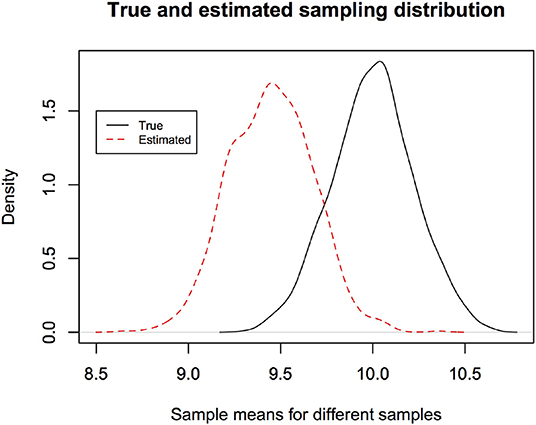
Figure 1. The estimated sampling distribution depends on the observed data and is different from the true sampling distribution. Hence the parameter estimate of a new study may lie outside the confidence interval reported in an earlier study more often than the nominal error rate. The new estimate is occurring from the true sampling distribution and the previous confidence interval is based on the estimated sampling distribution. It is approximately the area outside the reported confidence interval under the true sampling distribution.
Sampling distributions can be estimated using various other techniques, such as using pivotal statistics, asymptotic normal approximation, inversion of the likelihood ratio or by non-parametric bootstrapping (Casella and Berger, 2002). As an aside, the last two techniques are considered preferable because they lead to confidence intervals that are parameterization equivariant. That is, one can transform the confidence interval for μ to log(μ) by simply log-transforming the endpoints of the first interval. Although their lengths and end points will change, their coverage properties remain invariant. Thus, likelihood ratio based or bootstrap based confidence intervals satisfy desiderata 1 but confidence intervals based on other methods may not. We will discuss implications to other desiderata in the next section.
Let us look at how one can use the (true and estimated) sampling distribution for quantifying uncertainty about the inferential statements.
3.1.1. Confidence Intervals and Coverage
It is easy to see that we can use the true sampling distribution to compute an interval that indicates the range of estimates that one would obtain in replicated experiments with specific probability. For example, using the true sampling distribution which, in this case, can be analytically shown to be , we can give 90% confidence interval as where n denotes the sample size and σ = 1. The confidence interval shrinks as we increase the sample size. As we noted before, it is impossible to compute this interval in practice because the true parameter values are unknown. The true 90% confidence interval for a sample size 20 is given by (9.624341,10.37566). A corresponding estimated 90% confidence interval based on the estimated sampling distribution, for a specific sample, turns out to be (9.716948,10.460803). This is different from the true confidence interval because we replace true mean by the estimated mean. For different samples, one would get different confidence intervals because each sample leads to a different estimate of the mean. The reader can use the R program in the Supplementary Material to see how parametric bootstrap sampling distribution and associated confidence interval varies depending on the sample in hand. Note that each run of the program will lead to different confidence intervals than reported above.
It is clear what information the true 90% confidence interval provides. It says that if you repeat the experiment, your estimate will lie inside the true confidence interval 90% of times. Hence your result will contradict the original result only 10% times. But what information does the estimated confidence interval provide about the true value of μ? We can make the following statement about the value of μ: If we replicate the experiment 100 times and calculate the estimated 90% confidence interval for each replication, then ~90% of the intervals will cover the true value (that is, the true value will belong to the interval). Of course, any particular interval obtained from a single experiment may or may not contain the true value. This is the property of the procedure and not of the outcome of a single experiment. The interpretations of the true confidence interval (that can never be computed) and the estimated confidence interval are different.
Thus, we have answered the question, how often (in replicated experiments) would our interval cover the true parameter value of μ? This is called the coverage probability. Is this useful? We contend that this is the kind of probability we use in practice. For example, probability of an airplane crash on a take-off is say 1 in 10,000. This tells us nothing with certainty about what will happen on a particular flight; it may crash or it may not crash. However, we intuitively understand this uncertainty statement and are able to make decisions. It helps us behave in a rational manner. This is what Neyman called “inductive behavior” (Lehmann, 1995), behavior informed by the data.
Replicability of the conclusions: Another question explicitly addressed by the sampling distribution is: How replicable is our study? How likely is it that we would be contradicted by someone conducting similar experiment? This is sometimes crudely put as “Cover Your Ass” (CYA) statements. For example, suppose the first sampler publishes a confidence interval for the mean biomass in a given size quadrat. Then we can use the true sampling distribution to compute the probability that subsequent sampling of the biomass will yield a mean biomass estimate that will not belong to the first sampler's confidence interval and hence the first sampler's conclusions will be contradicted by the subsequent study. This probability is not the same as the coverage probability which is the property of the estimated confidence interval. For example, for the estimated sampling distribution in Figure 1 (dotted curve), the probability that a new sampler will get an estimate outside the estimated confidence interval (μL, μU), namely, , turns out to be, on an average, 0.24. This is larger than the nominal 10% excesses under the true sampling distribution. Of course, as the sample size increases, this problem goes away. We conjecture that this is one of the reasons of the replicability crisis in science (e.g., Ioannidis, 2012), namely incorrect interpretation of the confidence interval; the other, perhaps far more important, being model misspecification or the model from one study not being applicable to other studies.
Replicability of the conclusions is an essential component of the scientific validity of the conclusions. Aleatory probability based quantification of uncertainty clearly tries to address this concern. Not everyone, however, agrees that classical quantification of uncertainty is useful. It is claimed that not all experiments can (will) be replicated. For example, the critics ask: How do we quantify uncertainty of the event of a nuclear war? How do we replicate a time series of populations? We find this objection fundamentally vacuous because, by its very nature, modeling of a natural phenomenon using a statistical model assumes the possibility of replication of the experiment. If replication of an experiment is impossible, statistical modeling of such an experiment is also impossible, nay meaningless. Unfortunately, even if we accept the Classical approach to quantification of uncertainty in principle, there are problems when applied to inferential statements.
3.2. Conditional Inference and Post-data Uncertainty
Let us continue with the question of estimating the mean biomass in each management quadrat. Previously, we assumed that all quadrats were identical to each other. It is reasonable to think that each quadrat has different mean biomass that depends on the habitat covariates of that quadrat. Let us assume that Yi ~ N(Xiβ, σ). This is a simple linear regression through the origin model with a single habitat covariate and constant standard deviation.
Given the data, that now consist of (yi, xi) where i = 1, 2, …, n, the MLE of β is given by where the summation runs over i = 1, 2, …, n. Suppose, again unrealistically, that the standard deviation is known. The question now is: What is the uncertainty associated with the estimator of the slope β? Because of the Normality assumption, we can represent the uncertainty using the variance of the estimator. Surprisingly, there are two possible answers to this question.
1. Conditional variance: The standard answer in regression analysis, e.g., Ramsey and Schafer (2002), is . Notice that the variance of depends on σ but more importantly also on the observed values of the covariates x1, x2, …, xn. If the observed set of covariates are widely dispersed, the variance of is small whereas if the observed set of covariates are not dispersed, the variance is large. This is why, in planning ecological studies or constructing sampling designs, we aim to have high dispersion in the covariate values. To most researchers, this makes intuitive sense. With this, the true sampling distribution of is given by:
This measure of uncertainty assumes that the replicated experiments are such that the covariate values are identical to the ones in the original experiment, namely, xi, i = 1, 2, …, n. The only difference between the replicate experiments is in the values of the responses Yi, conditional on the original covariate values. This is why it is called “conditional variance.”
2. Unconditional variance: On the other hand, one can argue that because our study is an observational study, if we replicate the experiment the specific covariate values that different experimenters would observe are likely to be different. Thus, an argument can be made that when characterizing uncertainty we should account for the possible variation in the covariates as well. Let us assume that the covariate values arise from N(0, 1). That is, if we plot a histogram of the covariate values from all the management quadrats, it will have a bell shape. Under this assumption, it can be shown that, . This is the variation in that we will observe if we replicate the experiment where the covariate values are not fixed. This variation does not depend on the covariate values because their values across the replications are different and hence are averaged over. Because we do not condition on the covariate values, this is called “unconditional variance.” In this case, the true sampling distribution is (now, approximately) given by:
It is obvious that the length of the true confidence interval is constant in the unconditional case whereas it depends on the particular covariate composition in the conditional case. Using the distribution of , we can find that, for smallish sample sizes, about 60% of the conditional confidence intervals will be shorter than the unconditional intervals and as the sample size increases 50% of the conditional confidence intervals are shorter and 50% are longer than the unconditional confidence intervals.
These conditional and unconditional confidence intervals can be obtained in practice by using bootstrapping (Wu, 1986; Efron and Tibshirani, 1993). There are two different ways to conduct bootstrapping for regression. One is called pairwise bootstrap where we resample with replacement from the pairs (xi, yi). This leads to unconditional confidence interval. On the other hand, one can resample with replacement from the residuals denoted by and then generate the bootstrap samples using . Notice that in this bootstrap, covariate values are identical throughout the boostrapping procedure. This conditional (also called, residual) bootstrap leads to conditional confidence intervals. Notice that residual bootstrap procedure assumes that the linear regression model is the true model whereas the pairwise bootstrap procedure does not assume the correctness of the linear regression. Thus, pairwise bootstrap is model robust.
Both conditional and unconditional answers are mathematically correct (that is, they have correct coverage under the appropriate replication, conditional or unconditional) but which one is scientifically appropriate? It makes sense to use the conditional variance if we want to report uncertainty about the estimate that we obtained based on our own particular data. For example, if we happen to get a really good sample, that is, observed sample covariate values are highly dispersed, we should be fairly confident that our particular estimated slope is pretty close to the true slope. On the other hand, if we were unlucky and got a sample such that the covariate values were not very dispersed, we should not be too confident about the slope estimate being close to the true slope. The unconditional variance, on the other hand, seems to penalize a lucky experimenter and award an unlucky experimenter by averaging over their performances. But if we want to protect against possible contradiction by other experimenters, who will get different covariate values than what we observed, reporting the unconditional variance makes sense. The answer seems to be “it depends on the scope of the inference.”
This has puzzled, stumped and bothered the frequentist statisticians for a very long time (e.g., Fisher, 1955; Cox, 1958; Buehler, 1959; Royall and Cumberland, 1985; Casella and Goustis, 1995; among many other papers). We will let the reader read through these papers to see the full technical and scientific discussion. The ambiguity of when and how to condition has led to the study of relevant subsets, subsets of the sample space over which replication should be considered, along with conditioning on appropriate ancillary statistics and more. Much of this discussion revolves around uncertainty in the parameter estimates. These are statistical constructs. Although, intuition suggests that conditional inference is both mathematically correct and scientifically appropriate, there is no direct, operational way to justify the quantification of uncertainty about a statistical construct. Suppose we can relate the discussion to uncertainty about the observables then may be we can make such statements ascertainable in practice. Would the prediction accuracy help us decide if the conditional inference is “scientifically appropriate” without resorting to intuition alone?
3.3. Prediction and Prediction Intervals
Let us first look at how we can solve the problem of prediction and its uncertainty using the Classical approach (e.g., Lejeune and Faulkenberry, 1982). Let θT denote the true value of the parameter and let us assume that the model is correctly specified. The goal is, given the sampled data, to predict the new observation and associated prediction uncertainty. This could be equivalently translated into estimating either the density function f(y; θT), the corresponding cumulative distribution function (CDF) F(y; θT) or, more directly the inverse of the cumulative distribution function, the quantile function, . Let us look at the estimation of the density function.
3.3.1. Estimated Predictive Density
Given the data, we can simply replace the true, but unknown, parameter θT by its estimated value and use to obtain prediction intervals for a new observation.
Here superscript p indicates predictive and subscript est indicates estimated predictive density approach. This is certainly parameterization invariant (at least when MLE is used to estimate the parameter), as it should be, but depends on the transformation of the observable. These properties can be proved quite easily.
1. Let us reparameterize the density using ψ = g(θ) where g(.) is a one-to-one function. Then, we can write θ = g−1(ψ) where g−1(.) is the inverse function of g(.). The density is only a function of y and hence it follows that .
2. Let us do a data transformation where z = h(y). In this case, we have to use the Jacobian of the transformation (Casella and Berger, 2002) to get the density in terms of z. The density in terms of z is given by . The density in terms of z looks quite different. However, if z1 = h(y1) and z2 = h(y2), then P(Z ∈ (z1, z2)) = P(Y ∈ (y1, y2)). The prediction intervals are different but the probability content is the same.
This makes perfect sense: If we measure the variable on a different scale, the prediction interval should depend on that scale. For example, suppose population abundances are modeled as Log-normal distributions. Then, log-abundances are distributed as a Normal distribution. One can obtain prediction intervals for the log-abundances using Normal distribution properties and simply transform the end points using the exponential transform to get the prediction intervals for the abundances. Both these intervals, although numerically quite different, have exactly the same probability content under the respective distributions. The coverage probability of the prediction interval, the uncertainty quantification, remains invariant to the choice of the data transformation as well as the choice of the parameterization.
The major problem with the estimated predictive density is that it tends to be too optimistic in the sense that it gives prediction intervals that are too short and that do not have appropriate coverage properties. Notice here that the predictive error statement is aleatory and probeable (Taper et al., 2019), either by using cross validation or by independent experiments. One reason for bad coverage property of the estimated predictive density is that it does not take into account the estimation error in (e.g., Aitchison, 1975; Cox, 1975). There are many different approaches to account for the estimation error (e.g., Smith, 1998) each with its own pros and cons. One of the straightforward approaches (e.g., Hamilton, 1986) is based on accounting for estimation error by using the following.
3.3.2. Classical Predictive Density
Where is the asymptotically Normal sampling distribution of the estimator and is the usual estimated Fisher Information matrix (e.g., Casella and Berger, 2002; Ramsey and Schafer, 2002).
Notice that the integration is with respect to θ and not , which makes a clean, philosophically sound justification for this approach awkward. The estimated Fisher Information matrix can be replaced by the observed Fisher Information matrix (e.g., Efron and Hinkley, 1978). The above definition of predictive density, of course, assumes that the sampling distribution of can be well-approximated by the specified Normal distribution. One can, naturally, replace the asymptotic approximation of the sampling distribution by the bootstrap estimate of the sampling distribution (Harris, 1989). In the context of the linear regression problem discussed above, this immediately raises the question: “which sampling distribution” should we use for integration, conditional or unconditional? For example, a pairwise bootstrap for regression (Efron and Tibshirani, 1993) will lead to different predictive density than using the residual bootstrap (e.g., Wu, 1986). The first one leads to unconditional whereas the second one leads to conditional sampling distribution but assumes that the regression model is appropriate. A conditionally appropriate solution to this problem was provided by Vidoni (1995) where he uses the p*-approximation to the distribution of the MLE as suggested by Barndorff-Nielsen (1983). He also uses the Laplace approximation (Tierney and Kadane, 1986) to avoid the integration altogether. What properties are satisfied by the Classical predictive density?
Shen et al. (2018) (see also Lawless and Fredette, 2005; Schweder and Hjort, 2016) consider the prediction problem from the frequentist perspective in detail. They consider a general form of the predictive density, namely . where Q(θ) is any distribution on the parameter values of θ. The different predictive densities described above are particular cases of this general form with different Q(θ). For example, when we use the Classical predictive density following Hamilton (1986), we use . An important result they prove is that the Classical predictive density has correct coverage probabilities only if the estimated sampling distribution of has correct frequentist coverage (Shen et al., 2018, p. 130). They show that the predictive densities in the form similar to the ones defined above are superior to the estimated predictive density (which is nothing but using a degenerate Q(θ), degenerate at ) in terms of average Kullback-Leibler divergence and in terms of prediction error. They study parameterization invariance of the coverage in some cases. The conclusion is that it does not hold in general. The error probabilities (coverage properties) of these inferential statements are generally not parameterization invariant for small samples but they are parameterization invariant for large samples. This is because most estimators have sampling distributions that are asymptotically normal. If an estimator does not have asymptotically normal distribution, it is not clear if the parameterization invariance will hold true in such cases.
The predictive density for the linear regression through origin (also considered by Shen et al., 2018), using the conditional variance, is easy to derive and to justify by noting that:
where the second component in the variance is due to the estimation error of . This is how, generally, one obtains the prediction interval for linear regression (e.g., Ramsey and Schafer, 2002).
One can obtain an approximate predictive density based on the unconditional variance as:
An obvious comparison would be to see which density comes closest to the true density
See Figure 2 for a visual comparison between estimated, conditional and unconditional predictive densities (for a particular observed sample) along with the true predictive density. In the figure, we illustrate four different samples to show that sometimes estimated predictive density comes closer to the true density and sometimes it can be quite different, depending on how close the estimated parameters are to the true parameters. The general predictive density averages these different estimated predictive densities to get, on an average, better performance.
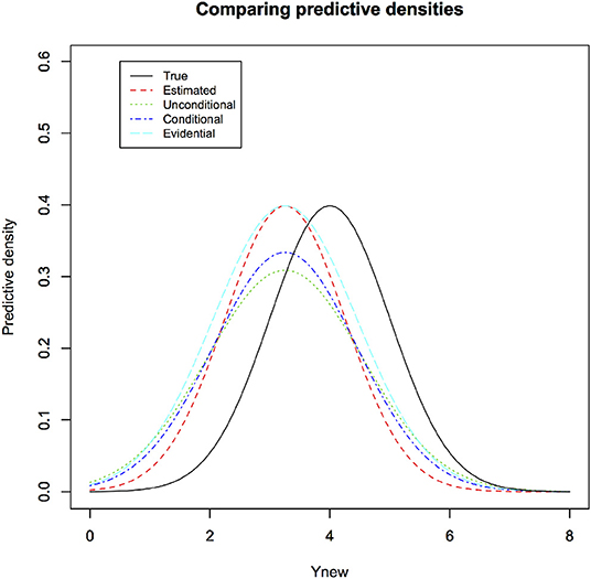
Figure 2. The true density for the new observation under the linear regression through origin is different than the estimated predictive density based on the observed data. Classical conditional, Classical unconditional have slightly fatter tails than the estimated predictive densities. This leads to somewhat better coverage properties by accounting for the sampling variability. Evidential predictive density also has fatter tails than estimated predictive density. Its calculation, however, does not need sampling distribution and hence specification of the experiment to be repeated. It reflects the information in the observed data appropriately.
Shen et al. (2018) compare the prediction coverage performance of the estimated, exact conditional and using the conditional bootstrap sampling distribution. In the Supplementary Material, we provide an R code that confirms that both conditional and unconditional predictive densities lead to correct predictive coverage of a future observation but conditional prediction intervals are shorter than the unconditional intervals when and longer otherwise. An immediate implication is that because conditional prediction intervals have correct coverage, when the unconditional prediction interval is shorter than the conditional prediction interval, it will have less than nominal coverage for those covariate configurations and when unconditional interval is longer than the conditional interval, it will have larger than nominal coverage for other covariate configurations. This implies that unconditional intervals are either unnecessarily conservative or incorrectly optimistic, but never correct conditionally (although correct on an average). This justifies the use of conditional variance in practical terms instead of “intuition.” See Royall and Cumberland (1985) for a similar argument in the context of finite population sampling. The differences between conditional and unconditional prediction intervals can be substantial when there are large number of covariates that leads to more variation in the covariate configurations.
3.4. What Should We Do?
It is clear that reporting the uncertainty in inferential statements about the parameters is tightly related to the question of “which experiment do we replicate?” Reporting the uncertainty about the parameters leads to the difficulties of “unconditional” vs. “conditional” (sometimes also termed pre-data and post-data) uncertainty. Because models and parameters are purely a statistical construct, the uncertainty statements related to their values are not justifiable directly and in practical terms. On the other hand, the observations have real world meaning. Reporting the uncertainty in statistical inference procedure in terms of its predictive accuracy is unambiguous. Thus, we can compare and contrast different uncertainty quantifications in terms of their predictive accuracy. For example, looking at the predictive accuracy, we can conclude that conditional predictive uncertainty is not only scientifically appropriate but also practically correct and better than the unconditional predictive uncertainty. Let us summarize what we can say about the Classical predictive density in the light of the desiderata from section 2.
1. The Classical predictive density is not parameterization invariant unless the sampling distribution is completely known, that is, it is a pivotal statistics (Shen et al., 2018). Sampling distribution based on the asymptotic normal approximation or the inversion of the Likelihood ratio test based on the asymptotic Chi-square approximation or bootstrapping leads to parameterization invariance of the predictive density. Thus, parameterization invariance is achieved only when valid bootstrapping of the data is possible or when the sample size is sufficiently large. However, bootstrapping time series or spatial data is not possible without some, possibly strong, additional assumptions.
2. Most of the results regarding the predictive density are proved under the assumption that the estimators are consistent and have asymptotically normal (CAN) distribution. However, in many complex ecological models, the conditions for CAN estimation may not be satisfied. For example, estimation of the boundary parameter commonly leads to estimators that are not CAN estimators. Such models may require non-standard asymptotics where the estimators approach the true value of the parameter at a rate different than or the asymptotic distribution may be different than Normal. It is unclear which of the above results hold true in such a situation.
3. The Classical predictive density does not automatically reflect how informative the observed data are. Unfortunately there is no general recipe to construct correct conditional or post-data sampling distribution for small samples. If one uses observed Fisher information (Efron and Hinkley, 1978) for the computation of predictive density, it appears to use the correct conditioning. See also Vidoni (1995) for appropriate conditioning in predictive density for small samples.
4. The Classical predictive density leads to correct predictive coverage only if the sampling distribution of has correct frequentist coverage properties. In general, the validity of the confidence intervals or prediction intervals can be rigorously proved only for large samples. Unfortunately, what is a large sample and if one has it in practice is never known. Whether or not a sample size is large, depends on the complexity of the model (e.g., Dennis, 2004).
5. Of course, even with proper conditioning under the presumed model, if the true regression model in the above example were non-linear or if the variance depended on the habitat covariates, the prediction intervals would have incorrect coverage.
6. Ideas, such as cross validation can be used to test the validity of the predictive density. Thus, these inferential statements are fully probeable.
7. Model estimation and model selection using cross validation, one of the most commonly used approach in much of machine learning literature, is based on computing the mean prediction squared error or some modification of it (e.g., Hastie et al., 2009). It is important to note that the method of cross validation, as is commonly used, is based on minimizing the unconditional prediction error as described earlier. This is troublesome. Furthermore, cross validation based model selection and Akaike Information Criterion (AIC) are closely connected to each other (Stone, 1977). However, Dennis et al. (2019) show that, according to the Evidential paradigm, use of AIC for model selection is problematic because the probability of misleading evidence does not converge to zero as the sample size increases.
8. Instead minimizing the MPSE, we suggest that one should check if the predictive density leads to appropriate prediction coverage. One could compare the predictive density with a non-parametric estimate (if such an estimation is possible) of the data generating mechanism, e.g., a non-parametric density estimate in the case of independent, identically distributed random variables. Any differences not only indicate that the model is incorrect but also can lead to model diagnostics and model correction.
In summary, the Classical approach satisfies some of the desiderata for the quantification of uncertainty. However, in order to get the sampling distribution, we have to address the crucial question of “which experiment do we repeat” and the answer is not straight forward.
4. Uncertainty Is All in Your Mind: Epistemic Probability for Quantification of Uncertainty
Classical uncertainty quantification is based on the properties of the procedures over replications of a specified experiment. Implicitly what is being claimed is that if the procedure is good on an average, the specific inferences are good as well. Of course, a good cook does not guarantee that a specific meal would be good; by chance, although rarely, you might get a bad meal. Is a specific inferential statement based on more accurate procedure better than one based on a less accurate procedure? For example, suppose we get exactly the same blood pressure (BP) measurement based on a drug store machine vs. in a doctor's office, should we take both of them equally at face value? Intuitively most would say no. However, not all statisticians agree with the quantification of uncertainty in terms of the accuracy of the procedure. They claim, because accuracy of the procedure is no guarantee that a particular inferential statement is good or bad, we cannot use it as a measure of uncertainty. They do not think it is epistemically correct to average over samples that we could have, but did not, observe. So how should we approach the question of quantification of uncertainty of a statistical inferential statement that reflect the lucky (or unlucky) observed data appropriately?
Bayesian approach assumes that, even before collecting the data, the experimenter is able to quantify their uncertainty about the value of the parameter. This may be based on prior experience about a similar situation, e.g., measurement error of the BP machine, distribution of the BP measurements in the population, prevalence of a disease, previous surveys in that study area, related surveys elsewhere or basic natural history of the species. Suppose one can quantify such prior belief in terms of a proper statistical distribution (that means it should be positive, countably additive, integrate or sum to 1 etc.). Such a distribution is called a “prior distribution.” This distribution describes the prior (to data) uncertainty about the parameter as quantified by the particular researcher. This is an epistemic uncertainty. This cannot be challenged nor can it necessarily be probed empirically. In this context, now we ask the question: In the light of the data, how do we change our prior beliefs (distribution)? Standard conditional probability calculation can be used to answer this question.
There are three components to every Bayesian analysis.
1. Prior distribution: Let θ denote the parameter of the model. This could be a vector indicating multiple parameters (as in multiple regression). Let Θ denote the parameter space, the set of values that the parameter can potentially take. We will generically denote the prior distribution by π(θ). This is assumed to be a proper statistical distribution. Thus, π(θ) > 0 for all θ ∈ Θ and ∫π(θ)dθ = 1.
2. Data generation model: This is the process model that postulates how the data are generated in nature. This is a statistical distribution on the observables. It varies for different values of the parameter. We will generically denote this by f(y(n)|θ) where y(n) = {y1,y2,…, yn} is the data vector.
3. Posterior distribution: The conditional probability distribution of the parameters given the data is called the posterior distribution. It is given by
We want to emphasize that, under the Bayesian framework, the model, as indexed by the parameter value, itself is a random variable. The prior distribution represents the researcher's belief about how probable a particular model is to represent the underlying process. This is an epistemic probability.
The posterior distribution completely quantifies the researcher's belief about the appropriateness of the model in representing the underlying process, after or in the light of the observed data y(n). Although the process model component is an aleatory probability, the posterior distribution, that combines epistemic and aleatory probabilities, is an epistemic probability.
In the Bayesian paradigm, the posterior distribution plays the same role that sampling distribution played in the Classical paradigm. Using the sampling distribution, we obtained confidence intervals that represented the range of estimated values that one may obtain if we replicate the experiment. Using the posterior distribution, one computes an interval that represents the experimenter's belief about the range of values that the true parameter could take. This is called a “credible interval.” There are no replicate experiments. Only one experiment was conducted and it resulted in the observed data. What changed, in the light of the data, are the prior probabilities about different parameter values. Just as the prior uncertainty was all in the mind of the experimenter, posterior uncertainty also is in the mind of the experimenter. See Brittan and Bandyopadhyay (2019) for a philosophical discussion on this point.
In Figure 3, we illustrate these three components for the linear regression through the origin example of section 3.2. We note that one can use credible interval to address the replicability of the inferential statement: How often do we believe we would be contradicted if someone replicates the experiment? The answer varies depending on the prior distribution. A credible interval does not have the interpretation of “how often would we cover the true parameter value if we repeat the experiment?” The uncertainty here is epistemic and is not testable.
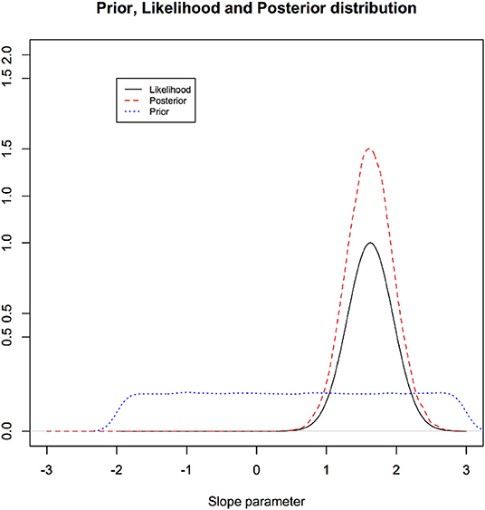
Figure 3. Illustration of a prior distribution, likelihood function, and posterior distribution for the linear regression through origin: notice how much the data can change the prior beliefs. Highly informative data change the prior substantially and vice versa.
Effect of the choice of the prior on the posterior distribution: It is obvious that if one has different prior beliefs, the posterior beliefs will be different even if the observed data are identical. In Figure 4, we illustrate how the posterior distribution changes with two different priors for the same observed data for the linear regression model considered earlier.
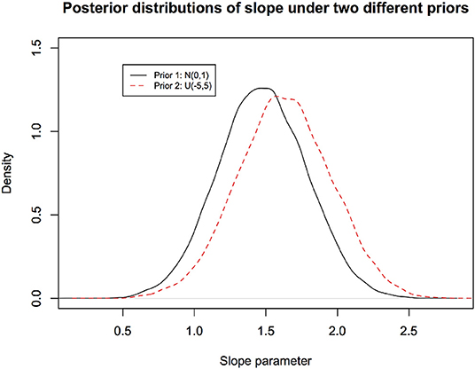
Figure 4. Different prior distributions lead to different posterior distributions. They both cannot possibly have correct frequentist coverage. Their validity is epistemic and is not testable in any practical fashion.
We invite the reader to play with the R code provided in the Supplementary Material to see how choice of the prior affects the posterior distribution.
We emphasize again that the posterior uncertainty does not reflect simply what the data says but reflects a combined effect of the prior beliefs and the information in the data. The probability statement reflected in the credible interval has no aleatory meaning. The uncertainty here is epistemic; it is neither testable nor verifiable in any fashion.
Note: A referee raised the possibility of checking the frequentist validity of the Bayesian credible intervals using the replicate experiments. Various researchers (e.g., Datta and Ghosh, 1995) have tried to study the frequentist validity of the Bayesian credible intervals. There are two problems with this comment.
• First problem is that the Bayesian credible intervals depend on the choice of the prior. This implies that not all priors can lead to credible intervals with good frequentist properties. We do not know if our particular choice of the prior will lead to good frequentist coverage. The research related to constructing priors that lead to correct frequentist coverage, called Probability Matching Priors (e.g., Datta and Ghosh, 1995), shows that it is extremely difficult to construct such priors, even for simple models and single parameter situation.
• Second problem is that if we are using the frequentist validity as a criterion for justifying Bayesian inference, we again face the difficulty of answering the question: which experiment do we repeat, conditional or unconditional? Would we be reporting proper post-data uncertainty? This justification violates the strong likelihood principle (e.g., Berger and Wolpert, 1988), that says that uncertainty should depend only on the data at hand and not on what other data one could have observed had the experiment been repeated, that Bayesian approach considers sacrosanct.
4.1. Bayesian Prediction and Prediction Uncertainty
As we did previously, it seems reasonable to relate the uncertainty statements to observables rather than the parameters facilitating testing and falsification in practice. We will describe the ideas under the assumption that the data are independent and identically distributed but they are easily extended to non-identically distributed or dependent data, such as space-time series of population abundances.
1. Prior predictive density: We can obtain Bayesian predictions even before obtaining any data. This is called a “prior predictive distribution.”
2. Bayesian predictive density: In the light of the data, the prior predictive distribution changes to posterior predictive distribution and is given by
where y(n) denotes the data vector of length n.
4.1.1. Parameterization and Bayesian Predictive Density
According to desiderata 1, uncertainty about prediction of the future observation should not depend on the parameterization used in the modeling. To our surprise, unless we are misunderstanding, Bjornstad (1990) seems to claim that the Bayesian predictive density is not generally parameterization invariant. Suppose the prior distribution is uniform distribution on the parameter space. Then, using Laplace approximation (Tierney and Kadane, 1986), one can write the Bayesian predictive density approximately as (Leonard, 1982):
where y(n) = y1, y2, …, yn, y(n+1) = y1, y2, …, yn, yn+1, is the MLE based on the data y(n) and is the MLE based on y(n+1). The matrix I(.) is the Fisher Information matrix. The non-invariance of the Information matrix to parameterization seems to make the Bayesian predictive density non-invariant to parameterization.
4.1.2. Sensitivity to the Choice of the Prior Distribution
It is obvious that as different priors lead to different posterior distributions, they also lead to different post-predictive densities. In Figure 5, we first depict the prior predictive densities induced by different priors along with the true density of the new observation for the linear regression model. It is clear that prior predictive densities or equivalently, induced priors on the observations (Lele, 2020) can be quite different from each other and the true density,
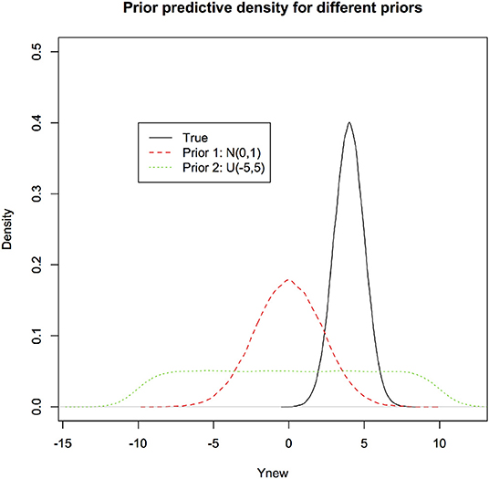
Figure 5. Prior predictive densities for the linear regression through origin example under two different priors. These represent the prior beliefs about the observation to be predicted. The true density (black) is presented for comparison. Prior predictive densities could be close to the true density if the prior distribution on the parameters is “good” and they can be very far if the prior distribution on the parameters is “inappropriate.” These are induced priors on the quantities of interest, namely values of the future data.
In Figure 6, we depict the Bayesian predictive densities corresponding to different prior distributions. The R code to produce these figures (with some Monte Carlo variation because the random numbers for each run are bound to be different) is provided in the Supplementary Material.
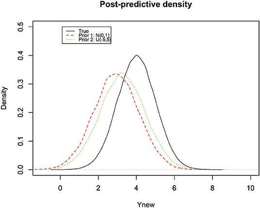
Figure 6. Bayesian predictive densities representing the post-data belief about the observation to be predicted. Notice how the effect of different priors has been reduced by the data. They are much closer to the true density (black curve).
The predictive coverage for these two Bayesian predictive densities corresponds to their overlap with the true density of the new observation. Given that Bayesian predictive distributions are sensitive to the choice of the prior distribution, they all cannot possibly have correct predictive coverage.
Shen et al. (2018) show that this predictive density will lead to good coverage only if the posterior distribution is also a valid frequentist sampling distribution. Given this result, it is obvious that Bayesian predictive density is unlikely to have correct coverage properties except in special circumstances or if the sample size is large enough to use the asymptotic Normal distribution approximation. Lawless and Fredette (2005) pointed out that objective Bayesian methods do not have clear probability interpretations in finite samples, and subjective Bayesian predictions have a clear personal probability interpretation but it is not generally clear how this should be applied to non-personal predictions or decisions. Similar objections were raised by many authors, e.g., Lele and Dennis (2009), Bandyopadhyay et al. (2016), Taper and Ponciano (2016), and Brittan and Bandyopadhyay (2019).
In statistical ecological literature (e.g., Royle and Dorazio, 2008; Kery and Royle, 2016) claims are made that Bayesian procedures are valid for all sample sizes without clear specification of the criterion for validity. It is clear that Bayesian prediction intervals do not have proper coverage as they should, at least in the aleatory sense. Perhaps the validity of the Bayesian procedures is also in the minds of the researchers.
4.1.3. Using Prior Data to Construct Prior Distributions
It may be tempting to think that using past data to construct prior distributions would be a way out of the subjectivity inherent in specifying a prior distribution. There are several problems with this approach. First, using past data implies that the past experiments are identical to the present experiment. If they are not, the estimates from the prior data cannot simply be put together in a histogram and use it to construct a prior distribution. This assumption may be satisfied in a few instances but not always. Suppose it is satisfied. In that case, a question one should ask: Is this the optimal way to utilize the past data? There is an alternative approach to utilizing the past data using the so called (ironically, indeed) “Empirical Bayes approach” or “Hierarchical models” or “Meta analysis” that does not involve constructing prior distributions from the results of the past experiments. We simply combine the likelihood functions of the past data with the likelihood function of the present data, under the assumption that the parameters of these different experiments are identical to each other or somewhat related to each other. This is likely to be statistically more efficient than reducing the past data to a prior distribution.
4.1.4. Model Checking
Model diagnostics is an essential component of any statistical analysis. Bayesian model diagnostics is usually based on the Bayesian predictive density. If the data are consistent with the Bayesian predictive (commonly called, post-predictive) density, it is taken as an indication that the model structure is appropriate. However, if the data are inconsistent with the Bayesian predictive density, a natural question to ask is: What part of the model is possibly incorrect? How should we modify it? Notice that the Bayesian predictive distributions (post- or pre-data) are mixture distributions (Lindsay, 1995). It is well-known (e.g., Teicher, 1961; Lindsay, 1995) that given observations from the predictive (mixture) density, one cannot uniquely determine the data generating (mixture components) distribution and the prior (mixture weights) distribution. Hence bad post-predictive fit does not tell us whether our prior distribution that is incorrect or the data generating mechanism that is incorrect and in what fashion. Even when the Bayesian predictive density fits the observed data well, it could very well be the case that both the prior distribution and the data generating mechanism are wrong but they compensate each other's mistakes to produce the correct Bayesian predictive distribution. Hence these post-predictive checks and model diagnostics are more ambiguous and less useful for scientific analyses than one would like them to be.
4.2. What Should We Do?
As long as one is willing to provide the prior distribution, the Bayesian approach to uncertainty quantification simply follows the laws of probability to obtain posterior beliefs about the parameters and predictive distributions. This appears to be a simple, elegant and logically coherent solution to the problem of uncertainty quantification.
An oft quoted, important result related to the Bayesian paradigm, is called the Complete Class theorem (e.g., Robert, 1994). In statistical decision theory, an admissible decision rule is a rule for making a decision such that there is no other rule that is always “better” than it, where the definition of “better” depends on the loss function. According to the complete class theorems, under mild conditions every admissible rule is a (generalized) Bayes rule (with respect to some prior distribution). Conversely, while Bayes rules with respect to proper priors are virtually always admissible, generalized Bayes rules corresponding to improper priors need not yield admissible procedures. Stein's example is one such famous situation (e.g., Robert, 1994). The main caveat that is, conveniently, not stated in the quantitative ecological literature, is that Complete Class Theorem is only an existence theorem and it does not instruct us which prior leads to the admissible estimator or how to construct such a prior. If your prior happens to be different than this optimal prior distribution, your results are likely to be suboptimal, if not downright misleading.
Let us look at the Bayesian prediction in the light of the desiderata presented in section 2.
1. Bayesian predictive density is not parameterization invariant unless the sample size is sufficiently large to wipe out the effect of the prior distribution. This lack of invariance can be problematic in practice (Lele, 2020). For example, one can (deviously) choose a parameterization such that Bayesian predictive distribution comes close to what one wants. This is the same as someone choosing a prior distribution to support pre-determined conclusions.
2. Bayesian predictive density automatically reflects how informative the observed data are. This is one of the attractive features of the Bayesian approach. It does not average over good and bad samples as the unconditional variance does in the Classical approach. Bayesian approach awards the researcher if the sample is informative and punishes when it is bad.
3. Bayesian predictive density does not lead to correct predictive coverage in general. This is obvious because different prior distributions lead to different post-predictive distributions. All of them cannot have correct predictive coverage. In general, the validity of the confidence intervals or prediction intervals can be rigorously proved only for large samples. What is a large sample and if one has it in practice is never known.
4. Ideas, such as cross validation can be used to test the validity of the predictive density. Thus, these inferential statements are fully testable.
5. If the post-predictive density does not appear to have good coverage properties, we cannot say whether it is due to the incorrect data generating mechanism or due to the prior distribution. Thus, it does not guide us to modify the data generating model. This is another important practical limitation of the Bayesian approach.
To summarize, in order to quantify uncertainty in the Bayesian paradigm one has to answer the question: What is the prior distribution? The Bayesian uncertainty statements reflect personal beliefs and hence are not transferable to anyone else, unless you happen to have the same prior beliefs. Uncertainty reflected in the posterior distribution has no aleatory meaning and hence is not probeable. Furthermore, predictive statements based on the Bayesian predictive densities are not guaranteed to have correct coverage. Another important limitation of the Bayesian approach is the lack of model diagnostics and suggestions for possible model modification. It can diagnose whether the model fits the observed data or not but, when the model does not fit the observed data, it cannot localize the errors in the model specification.
5. Evidential Paradigm and Quantification of Uncertainty
We will now study the Evidential paradigm and uncertainty quantification. For detailed introduction to the Evidential paradigm (see Royall, 1997). For an easily accessible and ecologically oriented version (see Taper and Ponciano, 2016 or Dennis et al., 2019). The Evidential paradigm is still in its infancy in terms of real life applications. However, we can observe certain general properties and study it in the light of the desiderata in section 2.
Royall (1997) claims that statistical inference addresses three different questions:
1. Given these data, what is the strength of evidence for one hypothesis vis-a-vis an alternative?
2. Given these data, how do we change our beliefs?
3. Given these data, what decision should we make?
Royall (1997) uses the likelihood function to quantify the strength of evidence in the data.
5.1. Likelihood Function
Suppose Y1, Y2, …, Yn are independent, identically distributed random variables with Y ~ f(.; θ) where θ ⊂ Θ. The likelihood function is given by: L(θ; y(n)) = ∏f(yi; θ). Recall that likelihood is a function of θ and the data y(n) = (y1, y2, …, yn) are considered fixed.
5.2. The Law of the Likelihood
Let θ1, θ2 denote two specific values of the parameters. Then the strength of evidence for θ2 vs. θ1 is given by the likelihood ratio
with values larger than 1 implying θ2 is better supported than θ1 and vice versa.
Strength of evidence can be seen to be a comparison of the divergence between the true model and the two competing hypotheses (Lele, 2004; Taper and Lele, 2004; Dennis et al., 2019; Ponciano and Taper, 2019). The law of the likelihood corresponds to using the Kullback-Leibler divergence but other measures, such as the Hellinger divergence, Jeffrey's divergence, etc. also lead to appropriate quantification of the strength of evidence with some important robustness properties (Lele, 2004; Markatou and Sofikitou, 2019).
The Evidential paradigm is fundamentally different from the Classical paradigm in that it concentrates not on the control of error probabilities but on the measure of distance of the proposed models (hypotheses) from the true model. See Taper et al. (2019) for further discussion. For example, one fixes a cut-off point K that indicates the strength of evidence (difference in the divergences) that will be considered “strong evidence” a priori. The choice of the value of K is of the experimenter. Given such a cut-off point, if the LR is larger than this cut-off point, we say that we have strong evidence for θ2. If it is < 1/K, then we say that θ1 has strong evidence. Anything in between, we say that we have weak evidence and neither hypothesis is strongly supported. For any fixed cut-off value, one computes probabilities of misleading evidence, weak evidence and study their behavior as sample size changes. In contrast to the Classical approach where probability of type I error remains fixed at the a priori level α, probabilities of both weak and misleading evidence converge to zero as the sample size increases. See the papers by Royall (2000) and Dennis et al. (2019) for more detailed discussion on this point. Evidential approach can be extended to the case of evidence for parameter of interest in the presence of nuisance parameters using the concept of profile likelihood (Royall, 1997; Royall and Tsou, 2003).
Much of the discussion above is in the context of comparing two specified parameter values. But it is easy to construct evidential intervals (e.g., Royall, 1997; Bandyopadhyay et al., 2016; Jerde et al., 2019) that provide a range of values that are “well-supported” by the data. This is, in spirit, similar to confidence intervals and credible intervals. Notice that these intervals reflect the information in the data appropriately: Highly informative data lead to shorter evidential intervals and vice versa in the regression example of section 3.
5.3. Evidential Intervals
Let us consider a single parameter case. An evidence interval for θ at level 1/K is given by:
for a fixed value of K > 0. This can be generalized to evidential sets for multi-parameter situation in a straight forward fashion.
How do we quantify uncertainty in the Evidential paradigm when the inferential statements are made about the parameters of the underlying process? The probabilities of misleading evidence, weak evidence and strong evidence as defined by Royall (1997) are pre-data quantities. He does not provide any explicit suggestions as to how to report the uncertainty of the strength of evidence once the data are obtained. Should one discuss coverage probabilities of evidential intervals? As we have argued throughout this paper, without such quantification of uncertainty, the inferential statements are incomplete. Taper and Lele (2011) attempt to answer this question using bootstrapping to compute the post-data error probabilities. Taper et al. (2019) use bootstrapping to compute the distribution over the range of values strength of evidence could have taken had the experiment been replicated. Such calculations seem to be enormously informative and useful in practice. However, any such calculation requires answering the same question that Classical paradigm faced: which experiment do we replicate? Hence, although Royall's formulation quantifies the strength of evidence that satisfies the likelihood principle (but see Lele, 2004), any computation of the uncertainty in the strength of evidence seems to face the same philosophical problems Classical paradigm faces. Do we gain anything by using the Evidential approach? An affirmative answer is provided in Dennis et al. (2019) in the context of model selection. Can we use prediction to resolve this problem in general?
The evidential paradigm can also be used for prediction using various versions of predictive likelihood (e.g., Bjornstad, 1990). Let us look closely at one such predictive likelihood (Mathiasen, 1979) and our suggestion for its modification. Following Shen et al. (2018), an intuitively appealing version of evidential predictive density may be defined as follows:
5.3.1. Evidential Predictive Density
Where yn+1 is the potential value of the new observation. It is necessary to assume that the integral in the denominator is finite. This may not be the case if the parameter space is infinite.
Evidential predictive density, in this formulation, is a weighted average of the data generating mechanism with weights proportional to the evidence for various parameter values in the observed data. This predictive density, in form, is identical to the predictive density one obtains with a uniform distribution as a prior distribution. However, if the parameter space is not finite, such a prior distribution is not mathematically valid as it does not integrate to 1. Let us look at the evidential predictive density a little more closely. First notice that the numerator is nothing but the likelihood function where data are now augmented by yn+1. Thus, the evidential predictive density can be written as:
Let denote the value of θ that maximizes L(θ; y(n+1)) and denote its Hessian, matrix of second derivatives, evaluated at . Similarly, let denote the value of θ that maximizes L(θ; y(n)) and denote its Hessian evaluated at . The difference in and is the effect of having a future observation equal to yn+1. Now we will use the Laplace approximation described in Tierney and Kadane (1986) to evaluate the evidential predictive density approximately as:
The evidential predictive density as defined above is not parameterization invariant (Bjornstad, 1990). Because Evidential predictive density and Bayesian predictive density are the same when one can impose a uniform prior distribution, this result also implies that Bayesian predictive density is not parameterization invariant in general. From a scientific perspective, it is clear that parameterization invariance is of fundamental importance (e.g., Bjornstad, 1990). See also Lele (2020) for practical consequences of lack of invariance in wildlife management.
Suppose we consider the part of the above approximation that is parameterization invariant as an estimate of the predictive density, namely,
In the following, we will call this as the evidential predictive density. Notice that the evidential predictive density is proportional to the predictive likelihood defined by Mathiasen (1979), namely . Bjornstad (1990) suggests using normalized version of the predictive likelihood, namely for predictive density and shows that it has good coverage properties. In our case, instead of the integral in the denominator, we use as an approximate normalizing constant.
Let us now look at our linear regression problem to see how the evidential predictive density compares with the true density of the new observation. Figure 2 illustrates the comparison between evidential predictive density and the true density for a new observation and for different sample sizes.
In the Supplementary Material, we have provided an R code that can be used to reproduce such a figure for different values of Xnew and other variations. It is clear from this figure that evidential predictive density is a reasonable, but not very accurate, approximation of the true density of the new observation. The area under the approximate Evidential predictive density is generally not equal to 1 and that may be the reason for the discrepancy. But such standardization breaks down the invariance property. The approximation, as expected, improves with sample size. An extensive simulation study of the performance of the Evidential predictive density involving various distributions, dependent data etc. will be needed to see if this approach is better than other approaches in terms of prediction coverage or density approximation. One can, however, study the properties theoretically. The likelihood for the parameter is only interpretable in a comparative fashion as a likelihood ratio. It will be interesting to see if the Evidential predictive density ratios, that correspond to profile predictive likelihood ratios, will approximate the true predictive density ratios.
5.4. Important Properties of the Evidential Predictive Density
1. In the following, we show that this estimator is a consistent estimator of the true density f(yn+1|y(n); θT). This is an essential property that has to be satisfied by all predictive densities. The result follows as long as the MLEs and are consistent estimators of θT, the true parameter value.
as n → ∞. This is a “pointwise convergence in probability” result. It would be useful to obtain a uniform convergence result.
2. The evidential predictive density is parameterization invariant. This follows by the parameterization invariance of the likelihood function.
3. The evidential predictive density, as defined above, does not require integration, numerical or otherwise.
4. The evidential predictive density is easy to use for dependent data, such as the time series or spatial data commonly occurring in ecology and other applied sciences.
5. The evidential predictive density uses neither the sampling distribution nor the posterior distribution of the estimator, thus avoids both the specification of the experiment that is to be repeated under the Classical paradigm or choice of the prior distribution that should be chosen under the Bayesian paradigm. Evidential predictive density depends only on specification of the data generating mechanism.
6. Dealing with random effects, missing data etc. is simply a prediction problem and hence evidential predictive density can be used for analyzing hierarchical models. Thus, this approach is applicable to many ecologically interesting problems.
7. The asymptotic validity of the evidential predictive density does not depend on the asymptotic sampling distribution or asymptotic posterior distribution. It only depends on the consistency of the MLE which is a much more relaxed assumption than existence of the asymptotic distribution.
8. The evidential predictive density is conditionally appropriate. It conditions on the appropriate ancillary statistics automatically by using the likelihood function in its entirety. Highly informative data lead to tighter prediction intervals and vice versa automatically.
9. The main disadvantage of the evidential predictive density, as defined above, is that it is not guaranteed to be a probability density function. That is, it may not integrate to 1 exactly when integrated over the range of Y. Given the consistency result, this is only a small sample problem. Initial simulations suggest that even for small samples, this may not be a major problem. Similar problem arises for some non-parametric density estimators based on orthogonal polynomials (e.g., Prakasa Rao, 1983) without causing many problems in practice. A simple solution is to normalize the predictive likelihood using . This integral exists if the range of Y is finite. Simulation results in Bjornstad (1990) suggest that predictive likelihood has good coverage properties for reasonable sample size.
10. It is not completely clear how to use general evidence functions in lieu of the likelihood function in the above formulation. If such an extension is possible, one may be able to make such inferences robust against outliers.
6. Conclusions
We studied three different ways to quantify uncertainty in inferential statements. We can summarize our findings as follows.
• Classical paradigm uncertainty quantification depends on deciding which experiment to replicate. Unfortunately this leads to problems related to the pre- vs. post-data uncertainty. The Classical uncertainty quantification does not always reflect what the data at hand says about the parameter or future observations. It averages the uncertainty over all possible realizations of the process and hence punishes those who happen to have good data and awards those with bad data. This is scientifically inappropriate.
• Bayesian paradigm eschews aleatory probability and uses epistemic probability to quantify uncertainty. Bayesian approach does not need to answer the question of which experiment to replicate and reflects the information in the data at hand without averaging over what other data might have been, but were not, observed. But it requires specifying a prior distribution. Specifying a prior distribution leads to the problems of subjectivity, aside from the specification of the data generating mechanism, and possibility of untestable mis-specification. The optimality claims about the Bayesian inference are somewhat vacuous because there is no general recipe to find the prior distribution that leads to such optimal decisions.
• The Evidential paradigm addresses the issue of conditioning on the observed data appropriately. It does not require hypothetical replications of the experiment to obtain uncertainty quantification about the observables. Evidential quantification of uncertainty is aleatory, and hence falsifiable in practice, that depends only on the data generating mechanism and the choice of the evidence function. One of the reasonable objections to the classical paradigm is that the idea of replication makes no sense when analyzing time series or spatial-time series data. However, evidential support intervals, error probabilities and evidential predictive density are applicable in a straight forward fashion to dependent data, hierarchical models and other more complex situations.
• The Evidential paradigm, unlike the Classical and Bayesian paradigm, has not been extensively field tested in wide range of practical situations. Its operational feasibility is largely unknown and needs to be explored. For some examples of its applications, see Jerde et al. (2019) for an important ecological application in the study of allometry and Taper et al. (2019) in model selection for linear regression analysis. Ironically, these applications point out that reporting the strength of evidence for different models needs to be bolstered by quantification of the reliability of the estimate of the strength of evidence. If this were to be the case in other situations, it will inevitably lead to the problem of addressing the question: which experiment do we replicate? and the associated conditionality conundrum. May be we have not escaped the shackles of the hypothetical replication of experiments when it comes to making inferential statements about parameters, a statistical construct. On the other hand, evidential predictive approach seems to satisfy most of the desiderata. Although promising, jury is still out for the evidential paradigm.
In conclusion, we show that to quantify uncertainty in statistical inference, one has to choose either a specification of the sampling distribution (conditional or unconditional) or a prior distribution on the parameters or an evidence function. As scientists and statisticians, we must understand and reflect upon the implications of each of these choices.
Data Availability Statement
All datasets generated for this study are included in the article/Supplementary Material.
Author Contributions
SL conceived of the project and conducted the analysis and writing of the paper.
Conflict of Interest
The author declares that the research was conducted in the absence of any commercial or financial relationships that could be construed as a potential conflict of interest.
Acknowledgments
The author thanks the insightful comments and various discussions he had with Mark L. Taper, Brian Dennis, and Jose M. Ponciano on the topic of foundations of statistical inference and ecology.
Supplementary Material
The R code for the simulations and figures are available at https://github.com/jmponciano/LELE_SophiesChoice.
References
Bandyopadhyay, P., Brittan, G., and Taper, M. (2016). Belief, Evidence, and Uncertainty. New York, NY: Springer.
Barndorff-Nielsen, O. (1983). On a formula for the distribution of the maximum likelihood estimator. Biometrika 70, 343–365.
Berger, J., and Wolpert, R. (1988). The Likelihood Principle. Hayward, CA: The Institute of Mathematical Statistics.
Billheimer, D. (2019). Predictive inference and scientific reproducibility. Am. Stat. 73, 291–295. doi: 10.1080/00031305.2018.1518270
Bjornstad, J. F. (1990). Predictive likelihood: a review. Stat. Sci. 5, 242–254. doi: 10.1214/ss/1177012175
Brittan, G. Jr., and Bandyopadhyay, P. S. (2019). Ecology, evidence, and objectivity: in search of a bias-free methodology. Front. Ecol. Evol. 7:399. doi: 10.3389/fevo.2019.00399
Buehler, R. J. (1959). Some validity criteria for statistical inference. Ann. Math. Stat. 30, 845–863.
Casella, G., and Berger, R. L. (2002). Statistical Inference. 2nd Edn. Pacific Grove, CA: Duxbury Press. 337–472.
Clark, J. S. (2005). Why environmental scientists are becoming Bayesians. Ecol. Lett. 8, 2–14. doi: 10.1111/j.1461-0248.2004.00702.x
Cox, D. R. (1958). Some problems connected with statistical inference. Ann. Math. Stat. 29, 357–372.
Cox, D. R. (1975). “Prediction intervals and empirical Bayes confidence intervals,” in Perspectives in Probability and Statistics, ed J. Gani (London: Academic Press), 47–55.
Datta, G. S., and Ghosh, J. K. (1995). On priors providing frequentist validity for Bayesian inference. Biometrika 82, 37–45.
Dennis, B. (2004). “Statistics and the scientific method in ecology (with commentary),” in The Nature of Scientific Evidence, eds M. L. Taper and S. R. Lele (Chicago, IL: University of Chicago Press), 327–378.
Dennis, B., Ponciano, J. M., Taper, M. L., and Lele, S. R. (2019). Errors in statistical inference under model misspecification: evidence, hypothesis testing, and AIC. Front. Ecol. Evol. 7:372. doi: 10.3389/fevo.2019.00372
Efron, B., and Hinkley, D. V. (1978). Assessing the accuracy of the maximum likelihood estimator: observed vs. expected Fisher information. Biometrika 65, 457–482.
Fox, C. R., and Ulkumen, G. (2011). “Distinguishing two dimensions of uncertainty,” in Perspectives on Thinking, Judging, and Decision Making, eds W. Brun, G. Keren, G. Kirkeboen, and H. Montgomery (Oslo: Universitetsforlaget), 21–35.
Hamilton, J. D. (1986). A standard error for the estimated state vector of a state-space model. J. Econometr. 33, 387–397.
Hastie, T., Tibshirani, R., and Friedman, J. (2009). The Elements of Statistical Learning. 2nd Edn. New York, NY: Springer.
Ioannidis, J. P. A. (2012). Why science is not necessarily self-correcting. Perspect. Psychol. Sci. 7, 645–654. doi: 10.1177/1745691612464056
Jerde, C. L., Kraskura, K., Eliason, E. J., Csik, S. R., Stier, A. C., and Taper, M. L. (2019). Strong evidence for an intraspecific metabolic scaling coefficient near 0.89 in fish. Front. Physiol. 10:1166. doi: 10.3389/fphys.2019.01166
Kery, M., and Royle, A. (2016). Applied Hierarchical Modelling in Ecology: Analysis of Distribution, Abundance and Species Richness in R and BUGS. New York, NY: Elsevier.
Lawless, F., and Fredette, M. (2005). Frequentist prediction intervals and predictive distributions. Biometrika 92, 529–542. doi: 10.1093/biomet/92.3.529
Lejeune, M., and Faulkenberry, G. D. (1982). A simple predictive density function. J. Am. Stat. Assoc. 77, 654–657.
Lele, S. R. (2004). “Evidence functions and the optimality of the law of likelihood,” in The Nature of Scientific Evidence, eds M. L. Taper and S. R. Lele (Chicago, IL: University of Chicago Press), 191–216.
Lele, S. R. (2020). Consequences of lack of parameterization invariance of non-informative Bayesian analysis for wildlife management: Survival of San Joaquin kit fox and declines in amphibian populations. Front. Ecol. Evol. 7:501. doi: 10.3389/fevo.2019.00501
Lele, S. R., and Dennis, B. (2009). Bayesian methods for hierarchical models: are ecologists making a Faustian bargain. Ecol. Appl. 19, 581–584. doi: 10.1890/08-0549.1
Leonard, T. (1982). Comment on “A simple predictive density function” by M. Lejeune and G. D. Faulkenberry. J. Am. Stat. Assoc. 77, 657–658.
Lindsay, B. (1995). Mixture models: theory, geometry and applications. NSF-CBMS Regional Conf. Ser. Probabil. Stat. 5, I-163.
Markatou, M., and Sofikitou, E. M. (2019). Statistical distances and the construction of evidence functions for model adequacy. Front. Ecol. Evol. 7:447. doi: 10.3389/fevo.2019.00447
Neyman, J. (1937). Outline of a theory of statistical estimation based on the classical theory of probability. Philos. Trans. R. Soc. Lond. A 236, 333–380.
Ponciano, J. M., and Taper, M. L. (2019). Model projections in model space: a geometric interpretation of the AIC allows estimating the distance between truth and approximating models. Front. Ecol. Evol. 7:413. doi: 10.3389/fevo.2019.00413
Ramsey, F., and Schafer, D. (2002). The Statistical Sleuth: A Course in Methods of Data Analysis. Belmont, CA: Duxburry Press.
Royall, R., and Tsou, T. S. (2003). Interpreting statistical evidence by using imperfect models: robust adjusted likelihood functions. J. R. Stat. Soc. B Stat. Methodol. 65, 391–404. doi: 10.1111/1467-9868.00392
Royall, R. M. (2000). On the probability of observing misleading evidence. J. Am. Stat. Assoc. 95, 760–768. doi: 10.1080/01621459.2000.10474264
Royall, R. M., and Cumberland, W. G. (1985). Conditional coverage properties of finite population confidence interval. J. Am. Stat. Assoc. 80, 355–359.
Royle, J. A., and Dorazio, R. M. (2008). Hierarchical Modeling and Inference in Ecology: The Analysis of Data From Populations, Metapopulations and Communities. London, UK: Elsevier.
Schweder, T., and Hjort, N. (2016). Confidence, Likelihood and Probability. Cambridge: Cambridge University Press.
Shen, J., Liu, R. L., and Xie, M. (2018). Prediction with confidence? A general framework for predictive inference. J. Stat. Plan. Infer. 195, 126–140. doi: 10.1016/j.jspi.2017.09.012
Smith, R. L. (1998). “Bayesian and frequentist approaches to parametric predictive inference,” in Bayesian Statistics, Vol. 6, eds J. M. Bernardo, J. O. Berger, A. P. Dawid, and A. F. M. Smith (Oxford, UK: Oxford University Press), 589–612.
Stone, M. (1977). An asymptotic equivalence of choice of model by cross-validation and Akaike's criterion. J. R. Stat. Soc. B Methodol. 39, 44–47.
Taper, M. L., Brittan, G. Jr., and Bandyopadhyay, P. S. (2019). Statistical Inference and the Plethora of Probability Paradigms: A Principled Pluralism. PhilArchive copy v2. Available online at: https://philarchive.org/archive/TAPSIAv2
Taper, M. L., and Lele, S. R. (2004). “The nature of scientific evidence: a forward looking synthesis,” in The Nature of Scientific Evidence, eds M. L. Taper and S. R. Lele (Chicago, IL: University of Chicago Press), 525–551.
Taper, M. L., and Lele, S. R. (2011). “Evidence, evidence functions and error probabilities,” in Handbook for Philosophy of Statistics, Vol. 7, eds M. R. Forster and P. S. Bandopadhyay (Amsterdam: Elsevier Press), 513–532.
Taper, M. L., and Ponciano, J. M. (2016). Evidential statistics as a statistical modern synthesis to support 21st century science. Popul. Ecol. 58, 9–29. doi: 10.1007/s10144-015-0533-y
Tierney, L., and Kadane, J. (1986). Accurate approximations for posterior moments and marginal densities. J. Am. Stat. Assoc. 81, 82–86.
Keywords: aleatory probability, conditional inference, empirical validation, epistemic probability, parameterization invariance, prediction, predictive densities, statistical paradigms
Citation: Lele SR (2020) How Should We Quantify Uncertainty in Statistical Inference? Front. Ecol. Evol. 8:35. doi: 10.3389/fevo.2020.00035
Received: 12 March 2019; Accepted: 06 February 2020;
Published: 13 March 2020.
Edited by:
Yukihiko Toquenaga, University of Tsukuba, JapanReviewed by:
Nathan Lemoine, Colorado State University, United StatesTore Schweder, University of Oslo, Norway
Copyright © 2020 Lele. This is an open-access article distributed under the terms of the Creative Commons Attribution License (CC BY). The use, distribution or reproduction in other forums is permitted, provided the original author(s) and the copyright owner(s) are credited and that the original publication in this journal is cited, in accordance with accepted academic practice. No use, distribution or reproduction is permitted which does not comply with these terms.
*Correspondence: Subhash R. Lele, c2xlbGVAdWFsYmVydGEuY2E=