Regression-based machine learning models for nitrate and chloride prediction in surface water in a small agricultural sand plain sub-watershed in southwestern Ontario, Canada

Machine learning (ML) models have proven to be an efficient technique for better understanding and quantification of surface water quality, especially in agricultural watersheds where considerable anthropogenic activities occur. However, there is a lack of systematic investigations that can examine the application of different ML regression models in agricultural settings to predict the surface water quality using a group of input variables, including hydrological (e.g., surface flow), meteorological (e.g., precipitation), and field (e.g., crop cover) conditions. In this study, multiple ML regression models, including support vector machine (SVM) and regression trees (RT), were employed on a 2-year dataset collected from a sand plain agricultural sub-watershed in southwestern Ontario, Canada (i.e., Lower Whitemans Creek) to predict the nitrate and chloride concentrations in surface water at nine sampling sites within the sub-watershed. The prediction capabilities of these ML models were determined using a group of evaluation metrics including the coefficient of determination (R²) and root-mean squared error (RMSE). In general, the Gaussian Process Regression (GPR) model was the optimal algorithm to predict the nitrate and chloride concentrations in surface water (R² was 0.99 and 0.98 respectively for training and testing). According to the results of a feature importance analysis, it was found that the field conditions (specifically the location of sampling site (main channel or tributary site) and crop cover) were the most crucial model input variables for accurate predictions of the output variables. This study underscores that ML regression models can be implemented to effectively quantify the water quality properties of surface water in agricultural watersheds using easily measurable parameters. These models can assist decision makers in advancing successful actions and steps towards protecting the available surface water resources.

1 Introduction

Surface water bodies (e.g., rivers, lakes, and streams) act as primary water resources for many communities, ecosystems, and activities including agriculture, fishing, and recreation (Gorgoglione et al., 2021). However, these systems are highly vulnerable to contamination from multiple natural contributors, including soil erosion, rock weathering, and decomposition of organic matter, and anthropogenic sources such as industrial discharge, urban stormwater, agricultural activities, and untreated wastewater (Akhtar et al., 2021; Marshall et al., 2022; Rixon et al., 2024). In addition, surface runoff from agricultural fields can elevate the concentration of nutrients (i.e., nitrogen and phosphorus species) in surface water due to the application of synthetic and manure-based fertilizers (Ha et al., 2020; Liang et al., 2020). These nutrients can degrade the surface water quality, leading to serious environmental problems such as algal blooms, oxygen depletion and eutrophication (Ahmed and Lin, 2021; Elsayed et al., 2021; Elsayed et al., 2022a). Such degradation of surface water quality has raised global concerns, leading to the establishment of national and international agreements and policies that aim to safeguard the available water resources. For example, the Canadian-U.S. Great Lakes Water Quality Agreement and Canada-Ontario Agreement on Great Lakes Water Quality and Ecosystem Health were issued to highlight the importance of considering the role of nutrient transport and dynamics on the water quality of the Great Lakes (Environment and Climate Change Canada, 2017; Environment and Climate Change Canada, 2021; Ministry of the EnvironmentConservation and Parks, 2021). In general, the obligations from different frameworks and policies are a crucial component of sustainable water resources management and environmental protection, emphasizing the importance of continuous water quality monitoring in watersheds.

Nitrate (${\text{NO}}_3^{-}$) is frequently reported to be exported from agricultural watersheds to surface water because it is highly soluble and mobile in water (Gardner et al., 2020; Elsayed et al., 2023a). Also, it can be easily leached from the soil matrix because it is highly stable and cannot be combined with other pollutants in water (Arabgol et al., 2016; Bedi et al., 2020). In addition, there are multiple contributors of chloride (${\text{Cl}}^{-}$) in agricultural watersheds including both natural (e.g., salts in rocks and soils, and atmospheric deposition) and anthropogenic (e.g., road de-icing salts, and soil fertilizers) sources. High ${\text{Cl}}^{-}$ levels in agricultural watersheds can adversely affect plant health and soil quality, negatively impacting agricultural yield and long-term soil productivity (Mackie et al., 2022; Syeed et al., 2023). Moreover, elevated ${\text{Cl}}^{-}$ concentrations in surface water can cause ecological imbalances in aquatic systems such as osmotic stress, acute and chronic toxicity for aquatic organisms (Castiblanco et al., 2023). Thus, ${\text{NO}}_3^{-}$ and ${\text{Cl}}^{-}$ concentrations serve as critical indicators for assessing the health of surface water in agricultural watersheds, magnifying the necessity of effective and continuous water quality monitoring of surface water bodies.

Continuous monitoring of these surface water quality parameters is crucial to effectively manage pollution sources and prevent the disruption of biodiversity and surface water quality. By collecting and maintaining advanced datasets on water quality parameters (e.g., ${\text{NO}}_3^{-}$ and ${\text{Cl}}^{-}$), decision makers can implement evidence-based policies and facilitate timely interventions to safeguard water resources (Chow et al., 2020; Persaud et al., 2023). However, conventional monitoring methods, especially in agricultural watersheds, are often limited by multiple challenges associated with sampling and logistical constraints (Bhattarai et al., 2021). For example, regular sampling across large and diverse regions is costly, time-consuming, and labor-intensive. In addition, logistical constraints often limit access to certain areas, especially during winter, heavy rainfall, and snowfall events, resulting in spatial and temporal gaps in water quality datasets. Most water quality parameters (e.g., nutrient and solid concentrations) also require standard laboratory measurement procedures to obtain the final concentrations which are costly, resource-intensive, and time-consuming for obtaining continuous time-series in agricultural watersheds. Such challenges and the need for vigilant water quality management has led to increased attention to innovative monitoring and predictive approaches aided by data-driven techniques using machine learning (ML) models.

Recently, ML models have emerged as a powerful tool to tackle the limitations of traditional surface water sampling and monitoring methods (Pandey et al., 2023). ML regression models can offer a scalable solution to predict water quality parameters using a variety of environmental predictors, such as climatological and hydrological conditions (Kim et al., 2021; Varadharajan et al., 2022). ML models can also effectively compensate for the lack of comprehensive sampling data and offer predictions that support realistic decision-making by imitating complex patterns from historical observations (Imani et al., 2021; Portuguez-Maurtua et al., 2022; Wang X. et al., 2022). Unlike typical mechanistic models, ML models can process extensive and complex datasets with diverse parameters, allowing for high-resolution predictions across both time and space (Elsayed et al., 2022b; Elsayed et al., 2023b). ML models are particularly well adapted to agricultural watersheds where contaminant concentrations are highly variable and influenced by multiple environmental factors.

Previous studies applied different ML regression models (e.g., support vector machine and ensemble models) to predict general surface water quality parameters such as ammoniacal nitrogen and suspended solids concentration (Ahmed et al., 2019), total dissolved solids (Shah et al., 2021), and Carlson’s Trophic State Index (i.e., a reservoir water quality index) (Chou et al., 2018). However, few studies reported ML investigations that focused on specific surface water quality parameters, such as ${\text{NO}}_3^{-}$ and ${\text{Cl}}^{-}$, within the unique context of agricultural watersheds under different meteorological, hydrological, and field conditions. Limited studies have focused on engaging ML regression models to describe and predict the water quality conditions in different agricultural watersheds (Jung et al., 2021; Wang S. et al., 2022). Other studies employed multiple ML classification and regression models to quantify nutrient concentrations in surface water in clay agricultural settings (Elsayed et al., 2023b; Elsayed et al., 2024a). Few studies have compared the ability of different individual ML regression models to reproduce field datasets of ${\text{NO}}_3^{-}$ and ${\text{Cl}}^{-}$ concentrations from sand plain agricultural watersheds using a range of environmental predictors (e.g., meteorological and field conditions).

Furthermore, many of the previous studies predicted or simulated only a single surface water quality parameter. For example, multiple ML regression models were employed to only predict the water quality index (WQI) (Asadollah et al., 2021; Kouadri et al., 2021; Khoi et al., 2022), concentration of chlorophyll a (Chang et al., 2021), and total phosphorus (Qiao et al., 2021). Other previous studies used only 1 ML algorithm to predict water quality datasets without considering other potential candidates of ML models for higher prediction accuracy. For example, some previous employed the multiple linear regression (MLR) (Ha et al., 2020; Qun’ou et al., 2021), artificial neural network (ANN) (Imani et al., 2021; Gorgoglione et al., 2021; Balson and Ward, 2022), self-organizing map (Yu et al., 2021), random forest (Wang et al., 2021; Behrouz et al., 2022), and ensemble models (Melesse et al., 2020; Zhang et al., 2022) to predict nutrient concentrations in surface water. This reflects a major knowledge gap about the applicability of different ML regression models and further the selection of optimal models to predict multiple water quality parameters based on systematic comparisons about the performance of these models. Ultimately, limited studies have explored the adaptability of ML models to seasonal and spatial variability in contaminant levels, which is particularly pronounced in agricultural landscapes.

The main objectives of this study are to: (1) examine the interdependence and correlations between different process parameters (e.g., meteorological conditions) and surface water quality (i.e., nitrate-nitrogen (${\text{NO}}_3^{-}$-N) and ${\text{Cl}}^{-}$ concentrations); (2) compare the ability of different ML regression models to predict ${\text{NO}}_3^{-}$-N and ${\text{Cl}}^{-}$ concentrations in surface water given a group of input variables (e.g., field conditions); and (3) perform a feature importance analysis on the model input variables to assess their significance on the prediction accuracy of the optimal ML models.

2 Study area and data collection

2.1 Site description

The available dataset was obtained from the Lower Whitemans Creek study area (LWC) which is an agricultural sub-watershed in southwestern Ontario, Canada (Figure 1). The sub-watershed is located near Burford, Ontario in the lower portion of the Whitemans Creek watershed (404 km² with a stream order of 6.0). The Whitemans Creek watershed is a tributary of the Grand River watershed (6,700 km²) in southwestern Ontario. The LWC sub-watershed has an approximate area of 63.5 km², and it is dominated by agricultural activities (73% of the total watershed area) including pasture and forages. The main crops in the sub-watershed include corn (36%), soybeans (17%), pasture/forages (15%), and winter wheat (6%) (AAFC, 2023). It should be noted that these percentages of crop cover are determined based on the total watershed area. Elevations in LWC range between 254 and 360 m with an average slope of 3.4% over the entire sub-watershed. The sub-watershed is considered the most water-stressed region with the highest agricultural irrigation demand in the entire Grand River watershed (Wong, 2011; Larocque et al., 2019). The surficial geology is mainly comprised of gravel and sand with limited silt to sandy silt areas in the southwest region. Further details about the site description can be found in previous investigations that intensively studied the sub-watershed (Osman, 2017; Larocque et al., 2019; Arce-Rodriguez, 2024; Zeuner et al., 2025).

Figure 1

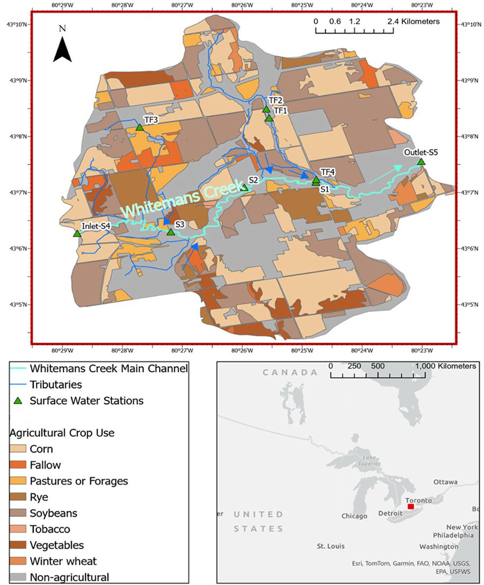
Figure 1. The Lower Whitemans Creek (LWC) sub-watershed in southwestern Ontario (Canada) with the five main observation sites on the main water course within the sub-watershed (i.e., S1 to S5) and four tributary observation sites (i.e., TF1 to TF4). The map shows the main river within the sub-catchment (i.e., Whitemans Creek). The background map, spatial data, and crop use were adopted from OpenStreetMap and Agriculture and Agri-Food Canada (AAFC) - Annual Crop Inventory (AAFC, 2023).

2.2 Dataset collection and description

In the current study, the available dataset was collected from five main observation sites that are located along the main channel (S1 to S5, S4 and S5 represents the sub-watershed inlet and outlet) (Figure 1). Also, the dataset was gathered from four observation sites (i.e., TF1 to TF4) that are located on tributaries (Figure 1). More details about the sampling sites, such as distance to the watershed outlet and geographic coordinates, are tabulated in Supplementary Table S1. The sampling campaign extended from October 2021 until the end of December 2023 for the main channel observation sites while the observation period of the tributary sampling sites ranged from August 2022 until the end of December 2023. Surface water was monitored monthly and sampled for water physico-chemical and quality parameters at these nine observation sites. These water physico-chemical parameters included the water temperature, dissolved oxygen (DO), pH, electrical conductivity (EC), and oxidation-reduction potential (ORP). The major surface water quality parameters were also monitored including the ${\text{NO}}_3^{-}$-N and ${\text{Cl}}^{-}$. Daily precipitation was monitored at the Brantford Airport Station that is close to the watershed outlet (approximately 5 km) (ECCC, 2021). The land use and crop cover were obtained from the actual agricultural activities during the observation period within the sub-watershed (AAFC, 2023).

The physico-chemical water parameters (e.g., water temperature and pH) were measured using a handheld multi-parameter instrument (i.e., YSI ProPlus). The surface water samples were collected from the center of the stream at a depth of approximately 0.40 m below the water surface for quantifying the water quality parameters. These water samples were gathered using clean high density polyethylene bottles which were stored on ice and then sent for analysis within a day of sampling. During the analysis of water quality parameters, the samples were filtered using 0.45 µm Fisherbrand Basix Syringe Filters then they were analyzed using a Metrohm Eco IC Ion Chromatograph at the Morwick G360 Groundwater Research Institute laboratory in the University of Guelph. The detection range of ${\text{NO}}_3^{-}$-N was 0.01–100 mg ${\text{NO}}_3^{-}$-N/L while the measurement error/detection accuracy was ±0.1 mg ${\text{NO}}_3^{-}$-N/L. For the ${\text{Cl}}^{-}$ measurements, the detection range and accuracy were 1–500 mg/L and ±1.0 mg/L, respectively. Precipitation was monitored in the Brantford Airport Station, that is operated by the Environment and Climate Change Canada - Meteorological Service of Canada, using an OTT-Pluvio² rain gauge that can measure both the rain- and snow-fall depth and intensity with a detection range of 0.1–200 mm/day and detection accuracy of ±0.2 mm (ECCC, 2021). The air temperature and water levels were measured using FTS THS-3 and Sutron Accubar Bubbler pressure sensors, respectively. The detection range varied between −50°C and 50°C for the air temperature and 0–5 m for the water level. The detection accuracy was ±0.1°C for the air temperature and ±0.5 cm for the water level. More details about the data collection can be obtained from other studies that investigated this sub-watershed (Arce-Rodriguez, 2024; Zeuner et al., 2025).

2.3 Hydrological and meteorological conditions

During the observation period (i.e., 1 October 2021 to 31 December 2023), the average daily stream flow ranged from 0.35 to 39.5 m³/s where the average daily stream flow over the observation period was 4.15 m³/s. The peaks of the stream flow were corresponding to snow-melt events in the winter and/or early spring over the entire observation period (Figure 2). For example, the highest stream flow (i.e., 39.5 m³/s) was recorded in early spring of 2023 (i.e., the first week of April). Other peak stream flows were observed in March 2022 and 2023, corresponding to snow-melt events. In addition, the daily average stream flow was high during the winter of 2022 and 2023 where it reached to approximately 16.3 m³/s in February 2023 (Figure 2). Over the observation period, the total precipitation was 1763 mm while the average of the total annual precipitation amount was approximately 785 mm. In general, the total rainfall depth was the highest in the fall of 2021 with a total depth of 311.3 mm while the fall of 2022 was the driest season over the observation period with a total rainfall depth of 108.3 mm (Figure 2). The highest daily total rainfall depth was recorded in the Summer of 2023 (i.e., July 2023) with a total depth of 43.5 mm. Following to this rainfall event, the second highest rainfall depths were 39.2 and 38.5 mm that were measured in February 2022 and April 2023, respectively, resulting in the highest stream flow records during the observation period. The average daily air temperature ranged between −17.6°C and 26.7°C over the observation period where the minimum and maximum air temperatures were observed in January and June 2022, respectively. In addition, there was no major variability in the annual pattern of the air temperature (similar to the sinusoidal wave) where the maximal and minimal air temperatures were approximately 24 and -14°C during the summer and winter, respectively (Figure 2).

Figure 2

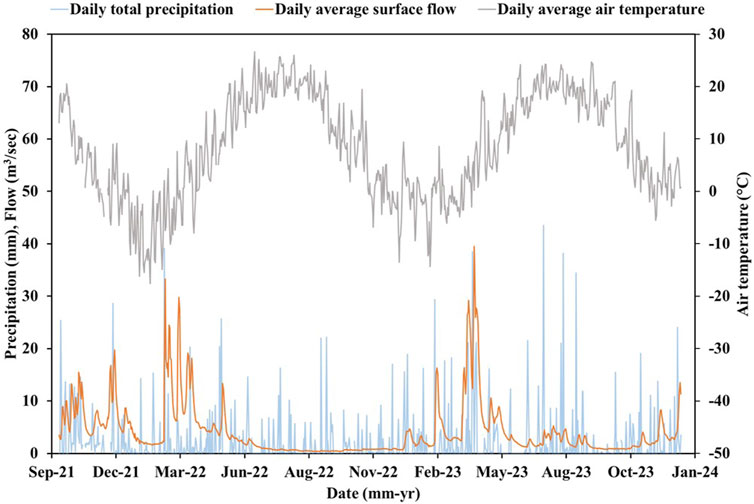
Figure 2. Daily average stream flow, total precipitation, and average air temperature during the observation period (1 October 2021 – 31 December 2023).

2.4 Surface water quality parameters

In the current study, the selection and classification of the measured water quality parameters followed established environmental standards and guidelines such as those outlined by the Canadian Water Quality Guidelines, the U.S. Environmental Protection Agency, and the World Health Organization. For example, the standard reference/acceptable limit of ${\text{NO}}_3^{-}$-N concentration in surface water was marked at 2.95 mg ${\text{NO}}_3^{-}$-N/L according to the Canadian Water Quality Guideline for the Protection of Aquatic Life (CWQGPAL) (Steele and Veliz, 2007; Canadian Council of Ministers of the Environment, 2011; Canadian Council of Ministers of the Environment, 2012). For the ${\text{Cl}}^{-}$ concentration in surface water, the standard reference was selected based on the guidelines determined by the Canadian Council of Ministers of the Environment (CCME) (CCME, 2011). According to the CCME, the aesthetic guidelines for drinking water was chosen to be 250 mg/L which was determined based on numerous considerations towards human health, ${\text{Cl}}^{-}$ taste thresholds, and the corrosion possibilities of the drinking water distribution networks and systems (Health Canada, 1987). The guidelines for the ${\text{Cl}}^{-}$ concentration in surface water were then revised to consider the protection of freshwater aquatic life, setting guidelines of 120 mg/L and 640 mg/L for chronic (short-term) and acute (long-term) toxicological effects, respectively (Health Canada, 1999; CCME, 2011). In general, these environmental standards and guidelines define the acceptable limits for water quality parameters in surface water and groundwater systems.

${\text{NO}}_3^{-}$-N concentration in surface water at the five main observation locations along the main water course (i.e., S1 to S5) ranged from 1.10 to 6.05 mg ${\text{NO}}_3^{-}$-N/L with an average of 3.78 mg ${\text{NO}}_3^{-}$-N/L (Figure 3a). These observations are consistent with the ${\text{NO}}_3^{-}$-N concentrations reported in other sand and silt plain agricultural watersheds (Tian et al., 2016; Sigler et al., 2018; Stelzer and Scott, 2018; Richards et al., 2021; Wang X. et al., 2022). However, they are relatively lower than the reported ${\text{NO}}_3^{-}$-N concentrations in surface water in a clay agricultural watershed in southern Ontario (Rixon et al., 2020; Mackie et al., 2021; May et al., 2023). This is mainly because clay soils have lower soil permeability, leading to slow water infiltration rate into the soil which increases the surface runoff that carry ${\text{NO}}_3^{-}$-N from fertilizers directly into surface water, leading to higher ${\text{NO}}_3^{-}$-N concentrations in surface water. In addition, tile drains, that are common in clay agricultural watersheds, represent a major source of ${\text{NO}}_3^{-}$-N transport into surface water (Rixon et al., 2020; May et al., 2023).

Figure 3

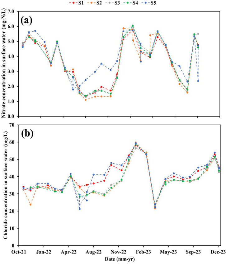
Figure 3. Surface water quality parameters at the five main observation sites (i.e., from S1 to S5) over the observation period (1 October 2021–31 December 2023): (a) ${\text{NO}}_3^{-}$-N, and (b) ${\text{Cl}}^{-}$ concentrations. Water quality datasets were collected by Arce-Rodriguez, 2024; Zeuner et al., 2025.

Moreover, the average ${\text{NO}}_3^{-}$-N concentration in surface water in the sub-watershed (i.e., 3.78 mg ${\text{NO}}_3^{-}$-N/L) is greater than the CWQGPAL limit (i.e., 2.95 mg ${\text{NO}}_3^{-}$-N/L) (Canadian Council of Ministers of the Environment, 2011; Canadian Council of Ministers of the Environment, 2012), emphasizing a considerable level of contamination in the surface water within LWC (Figure 3a). The ${\text{NO}}_3^{-}$-N concentrations in surface water at the five observation sites were consistent where the peak concentrations took place in November and December 2021 March 2022 as well as January, March, and December 2023, following snow-melt events during winter and early spring. Also, one ${\text{NO}}_3^{-}$-N concentration peak was observed in June 2023 following a rainfall and runoff event during the summer (Figure 3a). Such snow-melt and rainfall events are governing controllers on ${\text{NO}}_3^{-}$-N transport because it is highly mobile and dissolvable in water where it can be rapidly transported from the soil matrix to the main water course with high surface runoff conditions. These observations are comparable with the main outcomes of previous ${\text{NO}}_3^{-}$-N transport investigations in agricultural watersheds (Miller et al., 2015; Singh and Craswell, 2021; D’Haene et al., 2022; Yang et al., 2024).

${\text{Cl}}^{-}$ concentration in the surface water at the five observation sites on the main channel varied from 21.25 to 59.76 mg/L with an average of 38.40 mg/L (Figure 3b). These ${\text{Cl}}^{-}$ concentrations are comparable with those concentrations reported specifically in Ontario, Canada, and generally across North America (Steele and Aitkenhead-Peterson, 2011; Stets et al., 2018; Sorichetti et al., 2022; Castiblanco et al., 2023). In addition, the range of the ${\text{Cl}}^{-}$ concentration in the LWC sub-watershed is below the limits of the aesthetic guidelines for drinking water (i.e., 250 mg/L) and both the short- and long-term guidelines for aquatic life (i.e., 120 and 640 mg/L, respectively). For the five observation locations along the main channel, the ${\text{Cl}}^{-}$ concentrations were consistent where the peak concentrations were observed in January, March, and December 2023 when snow-melt events during winter and early spring took place (Figure 3b). These high concentrations of ${\text{Cl}}^{-}$ are probably linked to the winter since the application of road salt is commonly used in the sub-watershed during the snowfall events. In addition, salts from applying synthetic and manure-based fertilizers can contribute to the high ${\text{Cl}}^{-}$ concentrations in surface water in the sub-watershed (David et al., 2016; Merchán et al., 2018; Park et al., 2018). These observations are generally consistent with the main observations of previous studies pertaining to ${\text{Cl}}^{-}$ transport in stream water in different watersheds (Mullaney et al., 2009; Perera et al., 2013; Granato et al., 2015). This is also compatible with the fact that road salt is considered the main source of ${\text{Cl}}^{-}$ transport in different watersheds in north America especially the Great Lakes Basin (Chapra et al., 2009; Oswald et al., 2019; Mackie et al., 2022). Further observations about the ${\text{NO}}_3^{-}$-N and ${\text{Cl}}^{-}$ concentrations in surface water at the tributary observation sites be found in the Supplementary Material Section (Supplementary Figure S1).

3 Methods

3.1 Machine learning (ML) regression models

In the current study, 8 ML regression algorithms were trained and tested to predict the ${\text{NO}}_3^{-}$-N and ${\text{Cl}}^{-}$ concentrations in surface water in the sub-watershed using a group of input variables including meteorological, hydrological, field, and water physico-chemical parameters. These ML algorithms were the linear regression (LR) (Chou et al., 2018; El Bilali and Taleb, 2020), regression trees (RT) (Kuzmanovski et al., 2015; Qun’ou et al., 2021), support vector machine (SVM) (Cervantes et al., 2020; Xu et al., 2020), artificial neural network (ANN) (Hafeez et al., 2019; Kim et al., 2021), Gaussian process regression (GPR) (Richardson et al., 2017; Daemi et al., 2019), ensemble bagged trees (Zhang et al., 2022), ensemble boosted trees (Melesse et al., 2020), and random forest (Zhou et al., 2019) models. These models were selected because they are commonly used in the literature with a demonstrated history of accurate prediction capabilities and robust performance especially for small-sized datasets (Ashari et al., 2013; Aggarwal, 2016; Gondia et al., 2022). Each model relies on specific methodologies to predict the output variables where the suitability of each model depends mainly on the nature of the dataset and the possible detection of the interplay relationships between the model input and output variables. The main methodologies, applicability, advantages, and limitations of the employed ML regression models are briefly explained in the Supplementary Material Section.

3.2 Evaluation metrics of ML regression models

Five different evaluation metrics were applied to assess the performance of the 8 ML regression models in predicting the ${\text{NO}}_3^{-}$-N and ${\text{Cl}}^{-}$ concentration in surface water within the LWC sub-watershed. These evaluation metrics are the coefficient of determination (R²) (Equation 1), root mean squared error (RMSE) (Equation 2), mean absolute error (MAE) (Equation 3), mean absolute percentage error (MAPE) (Equation 4), and variance of errors (${\sigma }^2$) (Equation 5). These evaluation metrics were chosen for measuring the performance of the predictive models as they are commonly employed in previous ML regression studies (Kovacs et al., 2022; Sajib et al., 2023; Sajib et al., 2024). Further details about the definition and rational behind these evaluation metrics can be found in the Supplementary Material Section.

$R^2={\left[\frac{{\sum }_{i=1}^n\left(Y_i-\overline{Y}\right)\left({\widehat{Y}}_i-\stackrel{\sim }{Y}\right)}{\sqrt{{{\sum }_{i=1}^n\left(Y_i-\overline{Y}\right)}^2}\sqrt{{{\sum }_{i=1}^n\left({\widehat{Y}}_i-\stackrel{\sim }{Y}\right)}^2}}\right]}^2(1)$

$RMSE=\sqrt{\frac{{\sum }_{i=1}^n{\left(Y_i-\widehat{Y_i}\right)}^2}{n}}(2)$

$MAE=\frac{{\sum }_{i=1}^n\left|Y_i-\widehat{Y_i}\right|}{n}(3)$

$MAPE=\frac{1}{n}{\sum }_{i=1}^n\left|\frac{Y_i-\widehat{Y_i}}{Y_i}\right|(4)$

${\sigma }^2=\frac{1}{n}{\sum }_{i=1}^n{\left(e_i-\overline{e}\right)}^2(5)$

Where: $Y_i$ = observed (actual) output variable, $\widehat{Y_i}$ = predicted (modelled) output variable, $\overline{Y}$ = mean of the observed values of the output variable, $\stackrel{\sim }{Y}$ = mean of the predicted values of the output variable, $e_i$ = error (difference between observed and predicted output variable), $\overline{e}$ = average error between observed and predicted output, and $n$ = total number of observations.

3.3 Data analysis and pre-processing

In the current study, 200 observations were obtained from the main channel and tributary observation sites. Some of these observations were eliminated from the dataset because some parameters, such as water physico-chemical parameters, were not measured within these observations. Additional data pre-processing was applied on the observations to statistically remove the outliers of the model variables by employing the box and whiskers method through developing a box plot for each of the ML regression model input and output variables at the main channel (Figure 4a) and tributary (Figure 4b) observation sites. There were 121 remaining observations from the main channel and 40 remaining observations for the tributary sites. The total number of observations (161 observations) is of the same order of magnitude with those reported in other studies, ranging from 40 to 300 data points (Najah Ahmed et al., 2019; Bedi et al., 2020; Elsayed et al., 2023b; Sakizadeh et al., 2024; Subbarayan et al., 2024).

Figure 4

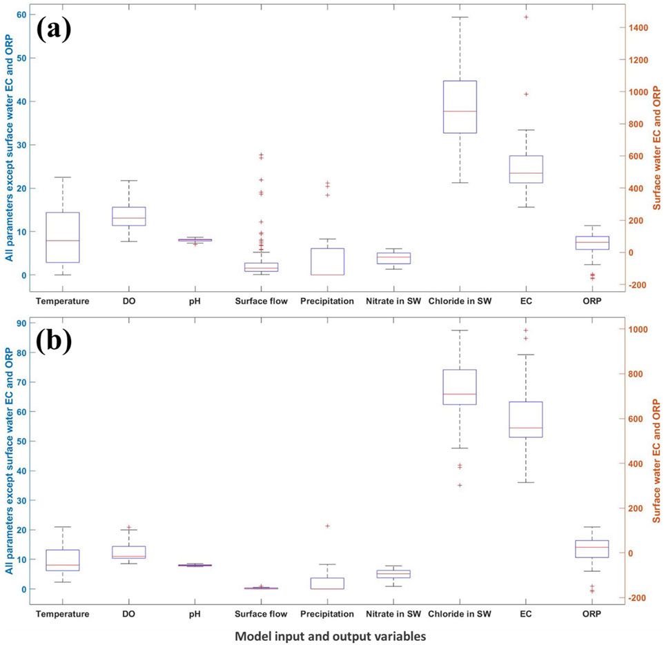
Figure 4. Box plot diagram for the surface water parameters using box and whisker approach for the: (a) main channel and (b) tributary sampling sites. * The units of surface water parameters are °C for temperature, mg/L for DO, m³/s for daily surface flow, mm for 24-h precipitation, mg ${\text{NO}}_3^{-}$-N/L for ${\text{NO}}_3^{-}$-N concentration, mg/L for ${\text{Cl}}^{-}$ concentration, μS/cm for EC, and mV for ORP.

The parameters of the available dataset were divided into four categories based on their relevancy and application in the ML regression models (Table 1). The first category includes the hydrological and meteorological conditions such as the daily flow rate and the daily precipitation on the day prior to the sampling. The second category contains field conditions such as the location of sampling sites (main channel or tributary) and the crop cover with a percentage of the three primary crops (i.e., corn, soybeans, and pasture) in the sub-watershed. The third category consists of field measured physico-chemical parameters including the water temperature, pH, DO, EC, and ORP. These three categories represented the input variables (i.e., features) of the ML regression models. These categories can enhance the ML model performance and predictive accuracy by accounting for hydrological, meteorological, and physico-chemical interactions influencing surface water quality. The fourth category involves the surface water quality parameters including ${\text{NO}}_3^{-}$-N and ${\text{Cl}}^{-}$ concentrations. In the current study, nitrate concentration represents nitrate-nitrogen (${\text{NO}}_3^{-}$-N) concentration in mg ${\text{NO}}_3^{-}$-N/L. The fourth category was chosen to be the model output variables to describe the most important and prevalent parameters that can reflect the surface water quality in the sub-watershed. ${\text{NO}}_3^{-}$-N and ${\text{Cl}}^{-}$ are key indicators of agricultural and anthropogenic influences on surface water quality. ${\text{NO}}_3^{-}$-N is a major contaminant associated with agricultural runoff and groundwater contamination while ${\text{Cl}}^{-}$ serves as a conservative tracer to reflect the natural sources (e.g., atmospheric deposition and salts in rocks and soils) and anthropogenic activities such as application of soil fertilizers and road salts.

Table 1

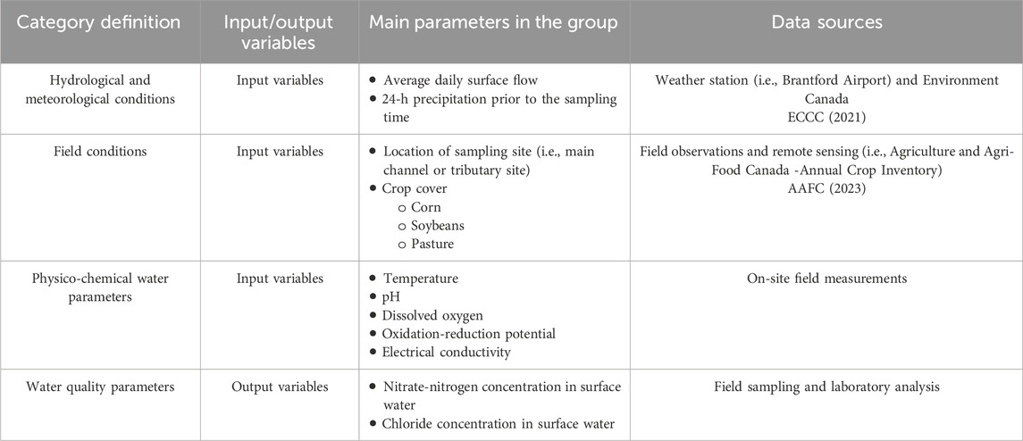
Table 1. Description of the main categories and parameters within the available dataset.

The total number of model variables used for the application of ML regression algorithms was 13 variables which is comparable with those reported in previous ML regression studies (between10 and 20 variables) (Knoll et al., 2019; Chang et al., 2021; Mosavi et al., 2021; Wang et al., 2021; Wells et al., 2021; Elsayed et al., 2022b). Here, the selected features are those listed in Table 1, including meteorological and hydrological, field, physico-chemical parameters as input variables, and water quality parameters as output variables. The observation period covered more than 2 years of monthly and event-based sampling where the temporal and spatial variations in the model features were measured. The sampling campaigns covered three successive non-growing and two successive growing seasons (from October 2021 to December 2023). This observation period is comparable with those reported in other ML investigations (Wagh et al., 2018; Islam et al., 2021; Perović et al., 2021; Yang et al., 2021).

The minimum ($X_{\mathit{Min}.}$), maximum($X_{\mathit{Max}.}$), average (mean) ($\overline{X}$), standard deviation ($\sigma$), coefficient of variation ($C_V$) and coefficient of skewness ($C_S$) were estimated for the model input and output variables (Table 2). Based on the statistical analysis, the highest coefficients of variation and skewness were corresponding to the daily average stream flow (188.1 and 3.63) and 24-h precipitation before sampling time (163.8 and 1.94), respectively. This is mainly due to the high variability in the meteorological and hydrological conditions in the LWC sub-watershed. Such variability was observed in other previous studies that investigated the hydrological response of watersheds in the Great Lakes Basin (Elsayed et al., 2023a; Elsayed et al., 2024a).

Table 2

Table 2. Main statistical parameters of the model input and output variables.

3.4 Modeling approach

Additional analysis was performed on some of the model input variables to prepare these features for the ML modeling. For example, the 24-h total precipitation prior to the sampling time was assumed to be uniform across the sampling locations (i.e., S1 to S5 and TF1 to TF4) within the sub-watershed for each observation. This assumption is based on the observations and local knowledge of the sub-watershed, which indicated no reported variations in snowfall or rainfall events that could disrupt the uniformity of precipitation across the nine observation locations. In addition, LWC is considered a small-sized catchment with minimal spatial variability in the meteorological conditions including the total precipitation. The stream flow rate at the observation sites was estimated using the watershed area ratio method (Gianfagna et al., 2015) since there was a lack of stage data at these observations locations which hindered the determination of surface flow rate by standard stage and rating curve techniques.

One of the key concerns in hydrological and water quality modeling is the potential collinearity between input variables which can lead to redundancy and affect the model performance. In particular, precipitation and stream flow are often correlated as precipitation serves since a primary driver of stream flow. However, in the current study, both variables were retained in the application of ML models because they capture distinct hydrological processes that contribute to water quality variability. Precipitation represents direct meteorological inputs while stream flow integrates multiple watershed responses, including antecedent soil moisture conditions, groundwater contributions, land use impacts, snow-melt events, and flow routing processes. Excluding stream flow from candidate model input variables can disregard its role as an aggregated hydrological response to various environmental drivers. In addition, most ML models (e.g., tree- and kernel-based models) are inherently more robust against multi-collinearity compared to simple ML models. By keeping both precipitation and stream flow in the analysis, it is ensured that ML models can learn from the full spectrum of hydrological variability, improving their predictive accuracy for the output variables.

For the crop cover, it was assumed to be uniform at all the sampling sites for each growing season, since the agricultural fields dominate the sub-watershed (approximately 73%) with similar crop patterns and distributions. For example, all sampling sites had a crop cover of 38, 37, and 11% for the soybeans, corn, and pasture, respectively, during the growing season of 2022 (i.e., from May to September 2022). For the growing season of 2023, the crop cover changed for all sampling locations to be 36, 17, and 15% for corn, soybeans, and pasture, respectively. During the non-growing seasons, the crop cover and percentage of each crop within the sub-watershed was considered to be zero where there were no agricultural activities in LWC during this period.

The previously mentioned model input variables, in Table 1, were employed to train the ML regression models to predict the output variables. The available dataset was divided into two sets where 70% and 30% of the dataset were used for the training and testing processes, respectively. Training process is used to familiarize the ML regression models with the input and output variables while considering the interplay between these model variables which assists in increasing the robustness of the ML regression models. Testing process is applied to determine the prediction accuracy of the ML model to estimate the output variables given new set of input variables.

Each ML regression model was used to predict a single output variable at a time (i.e., separate models for predicting ${\text{NO}}_3^{-}$-N and ${\text{Cl}}^{-}$ concentrations), considering the previously mentioned inputs variables in Table 1. For each ML regression model, the effect of the model hyper parameters was assessed to obtain the highest model prediction accuracy for each output variable. For example, the learner parameters, number of neurons, hidden layers, ensemble parameters were changed for the models to achieve the maximum model prediction capabilities expressed by the optimal evaluation metrics including R² and error indicators (e.g., RMSE and MAPE).

The main criteria of selecting the major research points relied on including a variety of input variables related to hydrological, meteorological, field conditions beside the physico-chemical water parameters to predict the ${\text{NO}}_3^{-}$-N and ${\text{Cl}}^{-}$ concentrations in surface water. The model input variables were chosen to be easily measured and quantified with minimal effort and time. In addition, the sampling locations were selected to capture the hydrological responses and nutrient dynamics in both the main and tributary sites, evaluating the spatial variability of nitrate and ${\text{Cl}}^{-}$ concentrations in surface water. These sampling locations were also chosen to examine the changes in ${\text{NO}}_3^{-}$-N and ${\text{Cl}}^{-}$ concentrations along the flow path in surface water, considering potential pollutant accumulation or dilution effects. Moreover, the observation period was more than 2 years with monthly sampling to identify the temporal variation of water quality parameters during the growing and non-growing seasons within the sub-watershed. For the model output variables, ${\text{NO}}_3^{-}$-N and ${\text{Cl}}^{-}$ were chosen due to their strong correlations with hydrological and field parameters while other water quality parameters (e.g., organic matter and microbial contamination) may not exhibit similar relationships with the selected input variables such as crop cover and management practices. Non-linear interactions and complex biogeochemical processes may require alternative modeling strategies beyond regression-based ML such as deep learning techniques and/or hybrid models (i.e., combination of process-based and data-driven models). In general, the selection of the model inputs and outputs was determined based on a combination of hydrological, geographical, and physico-chemical factors to ensure a comprehensive assessment of ${\text{NO}}_3^{-}$-N and ${\text{Cl}}^{-}$ concentrations across the sub-watershed.

3.5 Interdependence analysis

An interdependence analysis was performed by developing a correlation matrix between the model input and output variables to examine the degree of linearity and strength in relationships between the model variables. The correlation matrix, or correlation plot, serves as a key tool for identifying the relationships between different pairs of the model variables. Interdependence analysis is essential in complex processes, such as ${\text{NO}}_3^{-}$-N and ${\text{Cl}}^{-}$ transport to surface water, because the behaviour of each process parameter might be influenced by other parameters. In general, interdependence and correlation analyses aid in understanding the underlying mechanisms and relationships within the contaminant transport process and determining the crucial factors of the process which can enhance the prediction accuracy of ML models by eliminating the redundant variables. In these analyses, a high positive correlation between two model variables indicates a strong direct relationship, meaning that as one variable increases, the other also increases, and the reverse is correct when they decrease. On the other hand, a negative correlation reflects an inverse relationship, where a decrease in one variable is associated with an increase in the other. The interpretation of the correlation strength was determined based on commonly accepted limits and ranges in previous studies (Evans, 1996; Mukaka, 2012). Weak correlation can be defined when the correlation coefficient between a pair of model variables is less than 0.39. For moderate correlation, the correlation coefficient is ranged between 0.40 and 0.59 while strong correlation can be found when the correlation coefficient is greater than 0.60.

In the current study, the interdependence analysis was separately carried out on the main channel and tributary observation sites. In other words, the interdependence between the model variables was determined for each group of sites to examine the possible correlations between the process variables at different sampling locations. Thus, the process variables from the five main observation sites along the main water course (i.e., S1 to S5) were investigated to determine the potential correlation among these variables within the LWC sub-watershed. In another interdependence analysis, the process variables from the four tributary sites (i.e., TF1 to TF4) were examined and used for quantifying their possible correlations. For the interdependence and correlation analyses, the Pearson correlation coefficient was used to evaluate the strength and direction of the relationships between the model input and output variables. Pearson correlation is suitable for dealing with the water quality datasets that often exhibit linear relationships with other parameters such as hydrological and meteorological conditions. In addition, it was successfully adopted in multiple nutrient transport studies in the literature (Wagh et al., 2018; Elsayed et al., 2023b; Sajib et al., 2024). It is also commonly used for decision-making and water resources management because of its straightforward interpretation and practical applications (Sajib et al., 2023; Elsayed et al., 2024b; Uddin et al., 2024). In comparison to other correlation approaches (e.g., Spearman correlation), Pearson correlation can provide valuable insights about the magnitude of linear dependence between the model variables.

3.6 Feature importance analysis

In the current study, all candidate model input variables were initially included in the ML models, followed by a feature importance analysis (i.e., interpretability analysis) for these variables to assess their significance on the prediction accuracy of ${\text{NO}}_3^{-}$-N and ${\text{Cl}}^{-}$ in surface water using the optimal ML regression model. This approach can provide a more objective and comprehensive assessment of input variable contributions rather than relying solely on feature pre-selection based on prior assumptions (Knoll et al., 2019; Islam et al., 2021). Although some regression-based studies employ manual or stepwise selection methods before developing models, these methods can be sometimes subjective and biased. Also, such methods lack the consideration of the hidden patterns and nonlinear interactions among the environmental variables that can be unique to each dataset and watershed system. By first including a broad set of hydrological, meteorological, and field parameters, the ML models were exposed to all potential explanatory factors. Then, the subsequent feature importance analysis can aid in systematically ranking the input variables based on their predictive power, refining the model’s input selection (Wheeler et al., 2015; Harrison et al., 2021). This method enhances the interpretability of ML models and provides valuable insights into key drivers of water quality, which can be utilized in future monitoring and management strategies by stakeholders and decision makers (Messier et al., 2019).

This analysis was initially performed by omitting one input variable at a time to measure the influence of each input variable on the prediction accuracy of the optimal ML regression model (Table 3). These analyses were represented by scenarios from #1 to #9 in Table 3. Then, each group of input variables (i.e., hydrological and meteorological conditions, water physico-chemical parameters, field conditions) was removed to assess the impact of this group on the performance of the optimal ML regression models in predicting the output variables (Tables 1, 3). This group of simulations were referred as scenarios from #10 to #12 (Table 3). The feature importance analysis can generally assist in determining the governing factors on the accuracy of model predictions, recommending the superiority of specific input variables within the ${\text{NO}}_3^{-}$-N and ${\text{Cl}}^{-}$ transport processes.

Table 3

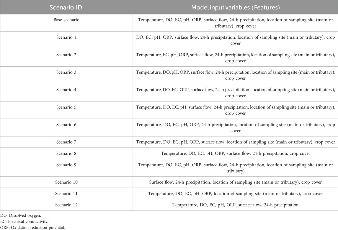
Table 3. The proposed feature importance scenarios using the optimal regression model and their corresponding model input variables.

Ultimately, the individual methodological steps of developing and validating the applied ML models for predicting ${\text{NO}}_3^{-}$-N and ${\text{Cl}}^{-}$ concentrations in surface water were described in a Figure 5. These steps included the dataset collection and pre-processing, identification of model parameters, correlation analysis, model selection, training, validation, and interpretation as well as the feature importance analysis. The details associated with each methodological step are highlighted in Figure 5.

Figure 5

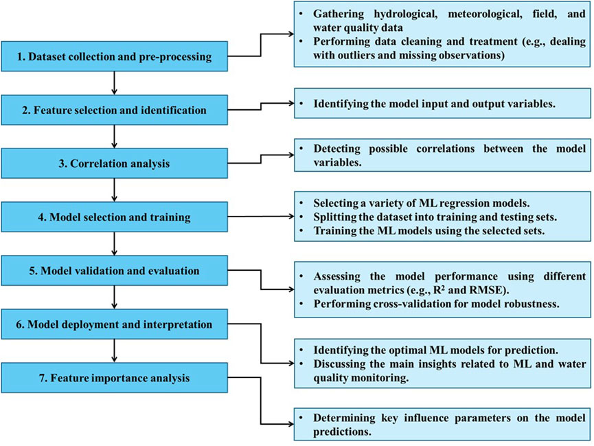
Figure 5. A flowchart for the individual methodological steps of applying the ML models.

4 Results and discussion

4.1 Interdependence analysis

For the five main observation sites along the main channel, there was no strong correlation between the ${\text{Cl}}^{-}$ concentration in surface water and the model input variables including the meteorological, hydrological, water physico-chemical, and field conditions (Figure 6). The range of correlation coefficients between measured ${\text{Cl}}^{-}$ concentration and model input variables was −0.42 to 0.22, indicating low interdependence between the ${\text{Cl}}^{-}$ concentration and the meteorological, hydrological, and field conditions in the LWC sub-watershed. This finding is comparable to the main outcomes of previous ${\text{Cl}}^{-}$ studies where it was found that the pathways of ${\text{Cl}}^{-}$ transport was controlled by anthropogenic drivers (e.g., road salt application) rather than meteorological variables and field conditions (Kaushal et al., 2005; Perera et al., 2013; Overbo et al., 2021). For example, some previous studies demonstrated that the degree of urbanization, ubiquity of septic systems in the watershed, presence of wastewater treatment facilities and land use type are the governing factors on the ${\text{Cl}}^{-}$ concentration in surface water (Betts et al., 2015; Lax et al., 2017; Overbo et al., 2021).

Figure 6

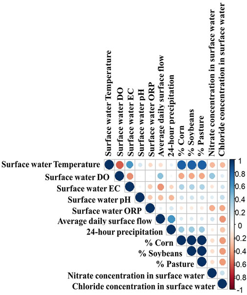
Figure 6. Correlation plot for the model input and output variables for the five main channel observation sites (i.e., S1 to S5).

Similarly to ${\text{Cl}}^{-}$ concentrations, ${\text{NO}}_3^{-}$-N concentrations at the five main channel observation sites were also not strongly correlated with the model input variables (Figure 6). The correlation coefficient between the ${\text{NO}}_3^{-}$-N concentration in surface water and other model input variables ranged from −0.32 to 0.38, indicating weak interdependence between ${\text{NO}}_3^{-}$-N concentration and these features. This observation is consistent with the outcomes of previous ${\text{NO}}_3^{-}$-N transport investigations where it was demonstrated that there were no clear relationships between ${\text{NO}}_3^{-}$-N concentrations in surface water and meteorological conditions, hydrological conditions, and field parameters (Wagh et al., 2018; Gorgoglione et al., 2021; Perović et al., 2021; Elsayed et al., 2023b; Elsayed et al., 2024a). However, some previous studies emphasized that the ${\text{NO}}_3^{-}$-N concentration in surface water is highly affected by the timing and amount of fertilizer application in agricultural fields (Rixon et al., 2020; Mackie et al., 2021; Singh and Craswell, 2021; D’Haene et al., 2022; Yang et al., 2024). In addition, the interplay between the different model variables and ${\text{NO}}_3^{-}$-N concentration in surface water might not be easily captured by the correlation matrix because these relationships are not strictly linear nor involve high interactions between the model variables. In other words, the relationships between the model variables are highly non-linear with multi-variable interactions.

For the model input variables, there was a strong positive correlation between the crop cover (i.e., percentage of the three primary crops in the sub-watershed) and surface water temperature with a correlation coefficient of approximately 0.82 (Figure 6). This is because the growing season in the LWC sub-watershed takes place mainly during the summer (i.e., starting from May to September) where the water temperature is relatively high. This observation is consistent with the outcomes from other studies that analyzed the interdependence between process variables in agricultural watersheds (Elsayed et al., 2023a; Elsayed et al., 2024a). Also, the 24-h precipitation prior to sampling time had a strong positive correlation (0.61) with the average surface flow because of the influence of rainfall and snowfall events on increasing the stream flow rate (Figure 2). In addition, the surface water temperature was inversely correlated with the surface water DO (−0.60) and directly correlated with EC (0.58). Ultimately, there were no strong correlations between the rest of the model input variables for which the correlation coefficients ranged from −0.44 to 0.46.

In general, there were no strong correlations between the model output variables, especially the ${\text{NO}}_3^{-}$-N concentration in surface water, and the model inputs as well as between the model inputs themselves, including the hydrological and meteorological conditions, and the field conditions. These unclear relationships between the model variables magnifies the importance of introducing ML regression models to describe the multi-dimensional interdependence between the process variables which enhance the understanding of the ${\text{NO}}_3^{-}$-N and ${\text{Cl}}^{-}$ transport processes.

4.2 ML regression models and the optimal models

Gaussian process regression (GPR) was found to be the optimal ML regression model to predict the ${\text{NO}}_3^{-}$-N concentration in surface water (Table 4; Figures 7a, b). The evaluation metrics of the GPR model were 0.99 for R², 0.30 mg ${\text{NO}}_3^{-}$-N/L for RMSE, 0.08 mg ${\text{NO}}_3^{-}$-N/L for σ², 0.21 mg ${\text{NO}}_3^{-}$-N/L for MAE, and 7.8% for MAPE during the training process. As for typical ML regression models, the model performance slightly decreased during the testing process where the evaluation metrics became 0.96 for R², 0.83 mg ${\text{NO}}_3^{-}$-N/L for RMSE, 0.68 mg ${\text{NO}}_3^{-}$-N/L for σ², 0.60 mg ${\text{NO}}_3^{-}$-N/L for MAE, and 17.1% for MAPE, albeit with an acceptable model prediction accuracy. The performance of the GPR model is comparable with the findings of other previous ML studies where R² $\ge$ 0.9 and MAPE $\le$ 20% reflected high prediction accuracy and robustness in the model performance (Bedi et al., 2020; Yang et al., 2021; Kovacs et al., 2022; Elsayed et al., 2024b).

Table 4

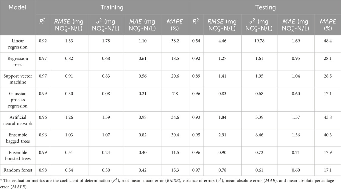
Table 4. Evaluation metrics of ${\mathrm{N}\mathrm{O}}_3^{-}$-N concentration in surface water using different ML regression models.

Figure 7

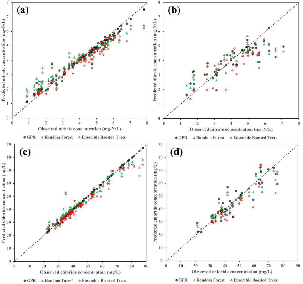
Figure 7. Regression plots for the optimal three algorithms for predicting the output variables: (a) training for ${\text{NO}}_3^{-}$-N concentration, (b) testing for ${\text{NO}}_3^{-}$-N concentration, (c) training for ${\text{Cl}}^{-}$ concentration, and (d) testing for ${\text{Cl}}^{-}$ concentration in surface water.

The ensemble boosted trees and random forest models yielded high prediction accuracy for the ${\text{NO}}_3^{-}$-N concentration in surface water (Table 4; Figures 7a, b). The evaluation metrics of the ensemble boosted trees were 0.99 for R², 0.51 mg ${\text{NO}}_3^{-}$-N/L for RMSE, 0.24 mg ${\text{NO}}_3^{-}$-N/L for σ², 0.40 mg ${\text{NO}}_3^{-}$-N/L for MAE, and 11.5% for MAPE for the training purposes while they decreased to 0.96 for R², 0.90 mg ${\text{NO}}_3^{-}$-N/L for RMSE, 0.72 mg ${\text{NO}}_3^{-}$-N/L for σ², 0.71 mg ${\text{NO}}_3^{-}$-N/L for MAE, and 17.9% for MAPE during the model testing. For the random forest model, the training and testing evaluation metrics were 0.98 and 0.97 for R², 0.54 and 0.78 mg ${\text{NO}}_3^{-}$-N/L for RMSE, 0.30 and 0.61 mg ${\text{NO}}_3^{-}$-N/L for σ², 0.42 and 0.60 mg ${\text{NO}}_3^{-}$-N/L for MAE, and 15.3% and 17.1% for MAPE, respectively. In multiple previous studies, the ensemble boosted tree and random forest models showed strong prediction capabilities in predicting the water quality parameters such as ${\text{NO}}_3^{-}$-N and phosphorus concentrations (Harrison et al., 2021; Aldrees et al., 2022; Farazan et al., 2024; Zheng et al., 2024), confirming their robustness in predicting the output variables in the current study. The ensemble boosted trees and random forest models generally gave close descriptive accuracy to the one of the GPR model for predicting the output variables. However, the GPR model showed higher superiority and a more robust performance especially in the training process.

The rest of adopted ML regression models showed high prediction capabilities of ${\text{NO}}_3^{-}$-N concentrations during the training process where the range of evaluation metrics was 0.92–0.97 for R², 0.82–1.33 mg ${\text{NO}}_3^{-}$-N/L for RMSE, 0.68–1.78 mg ${\text{NO}}_3^{-}$-N/L for σ², 0.56–1.10 mg ${\text{NO}}_3^{-}$-N/L for MAE, and 18.5%–38.2% for MAPE (Table 4). During testing, the performance of these models declined in predicting the ${\text{NO}}_3^{-}$-N concentrations where the evaluation metrics ranged from 0.54 to 0.96 for R², 1.27–4.46 mg ${\text{NO}}_3^{-}$-N/L for RMSE, 1.61–19.78 mg ${\text{NO}}_3^{-}$-N/L for σ², 0.95–1.69 mg ${\text{NO}}_3^{-}$-N/L for MAE, and 28.1%–48.4% for MAPE (Table 4). The linear regression model had the least good performance among the applied ML regression models. This is mainly because the linear regression model was not completely compatible with the nature of dataset where the model did not have the capabilities to capture the complex relationships between the model variables. Also, the linear regression model is a simple regression approach which is not suitable for the LWC dataset that has many parameters with high non-linearity and uncertainty.

The GPR, ensemble boosted trees, and random forest also gave the best performance in predicting the ${\text{Cl}}^{-}$ concentrations (Table 5; Figures 7c, d). The optimal ML regression algorithm was the GPR model where the evaluation metrics were 0.99 for R², 0.44 mg/L for RMSE, 0.19 mg/L for σ², 0.26 mg/L for MAE, and 0.7% for MAPE during the model training while they were reduced to 0.98 for R², 5.51 mg/L for RMSE, 31.08 mg/L for σ², 3.73 mg/L for MAE, and 8.4% for MAPE for the testing process. During the model training, the evaluation metrics of the random forest and ensemble boosted tree models were 0.99 for R², 3.12 and 4.14 mg ${\text{NO}}_3^{-}$-N/L for RMSE, 9.84 and 13.62 mg/L for σ², 2.01 and 2.83 mg ${\text{NO}}_3^{-}$-N/L for MAE, and 4.8% and 6.1% for MAPE, respectively. These values decreased during the model testing for the random forest and ensemble boosted trees to be 0.99 and 0.98 for R², 4.51 and 6.72 mg ${\text{NO}}_3^{-}$-N/L for RMSE, 20.8 and 38.96 mg/L for σ², 3.61 and 4.96 mg ${\text{NO}}_3^{-}$-N/L for MAE, and 8.4% and 10.3% for MAPE, respectively. The three models were common for yielding the best prediction accuracy of ${\text{NO}}_3^{-}$-N and ${\text{Cl}}^{-}$ concentrations because they were trained using the same input variables which were compatible with the nature of the dataset and the involved process variables.

Table 5

Table 5. Evaluation metrics of ${\mathrm{C}\mathrm{l}}^{-}$ concentration in surface water using different ML regression models.

Similar to the prediction of ${\text{NO}}_3^{-}$-N concentration in surface water, the linear regression was the least good model for predicting the ${\text{Cl}}^{-}$ concentrations especially during the model testing where the evaluation metrics were 0.66 for R², 38.47 mg/L for RMSE, 1,473 mg/L for σ², 11.95 mg/L for MAE, and 28.7% for MAPE. The remaining ML regression model gave good prediction accuracy during the training process where the range of evaluation metrics was 0.99 for R², 5.10–6.02 mg/L for RMSE, 26.04–36.5 mg/L for σ², 3.02–4.71 mg/L for MAE, and 7.2%–9.3% for MAPE (Table 5). For the model testing, the performance of these models slightly decreased where the evaluation metrics ranged from 0.96 to 0.98 for R², 5.51–9.67 mg/L for RMSE, 31.08–95.66 mg/L for σ², 3.73–5.95 mg/L for MAE, and 10.9%–12.8% for MAPE.

The selected 3 ML regression models (i.e., GPR, ensemble boosted trees, and random forest) showed a high prediction accuracy of the output variables where the predicted ${\text{NO}}_3^{-}$-N and ${\text{Cl}}^{-}$ concentration were well-scattered around the 45°-line in the regression plot especially for the training process (Figure 7). It should be mentioned that the GPR model was the most accurate model in predicting the output variables especially during the model training which was reflected on the evaluation metrics and the regression between the observed and predicted ${\text{NO}}_3^{-}$-N and ${\text{Cl}}^{-}$ concentrations. The GPR model also showed the least deviation of the 45°-line regression line compared to the rest of potential models (Figure 7). However, for the model training using ${\text{NO}}_3^{-}$-N concentrations as the model output, the ensemble boosted tree and random forest models tended to underestimate the ${\text{NO}}_3^{-}$-N concentration up to 4.0 mg ${\text{NO}}_3^{-}$-N/L while they overestimated the ${\text{NO}}_3^{-}$-N concentrations higher than 4.0 mg ${\text{NO}}_3^{-}$-N/L (Figure 7). A similar trend was observed during the model training using ${\text{Cl}}^{-}$ concentrations where the ensemble booted tree and random forest models overestimated the ${\text{Cl}}^{-}$ concentrations larger than 70 mg/L. Such underestimations and overestimations decreased the R² values and increased the error metrics of the two models compared to GPR during the training processes, confirming that the GPR algorithm was the optimal ML regression model for predicting the two output variables.

Such underestimations and overestimations are clear at either extremely low or high ${\text{NO}}_3^{-}$-N and ${\text{Cl}}^{-}$ concentrations where these values represented the two ends of the normal distribution of the dataset (i.e., 5% end of the distribution). These extreme data points were relatively limited and less present in the model training process compared to the concentrations near the median of the normal distribution. Moreover, most of the ML regression techniques inclined towards predicting the output variables closer to the mean of the target distribution which lowers the model prediction accuracy at the extremely high values. In addition, these models can sacrifice the variance to achieve high prediction accuracy as well as low RMSE value (Li et al., 2020). Moreover, the relationships between model inputs and outputs are different at the extremes compared to those near the mean values in many cases, deteriorating the model prediction accuracy at the extremes. To overcome these challenges associated with the extremes, more observations of these values can be collected and included in the training datasets which can improve the training capabilities of the ML models at the extremes.

Although the evaluation metrics of the ensemble boosted tree and random forest models were comparable with those obtained by the GPR model, they were not able to completely capture the actual variabilities in the ${\text{NO}}_3^{-}$-N and ${\text{Cl}}^{-}$ concentrations especially during the training process (Figure 7). The GPR model was able to perfectly capture the variability in ${\text{NO}}_3^{-}$-N and ${\text{Cl}}^{-}$ concentrations with the input variables over the observation period at the five main and four tributary observation locations where the predicted and observed concentrations were aligned on the 45°-line of the regression plot (Figure 7). This indicates the robustness of the GPR model in tracing the variations in the output variables under different conditions of the input variables.

4.3 Feature importance analysis

The GPR model was selected for the feature importance analysis since it was the optimal model for predicting the ${\text{NO}}_3^{-}$-N and ${\text{Cl}}^{-}$ concentrations in surface water. Accordingly, it was found that the R² value was not changed across the proposed scenarios during the testing process except for Scenario #8, 11, and 12 when the location of the sampling site (i.e., main channel or tributary), hydrological and meteorological conditions (i.e., average flow rate and 24-h precipitation), and field conditions (i.e., location of the sampling site and crop cover) were omitted from the input variables, respectively (Table 6). The R² value slightly decreased from 0.96 for the base scenario (i.e., including all the input variables) to 0.94 for Scenario #8 and 12 and 0.95 for Scenario #11 (Table 6). In addition, the error metrics (e.g., RMSE and MAPE) corresponding to these scenarios were relatively larger than those of the base scenario. For example, the MAPE value increased to 20.9% for Scenario #8, 20.1% for Scenario # 11, and 21.3% for Scenario #12 compared to the base scenario that had a MAPE value of 17.1% (Table 6). This highlights the importance of including the location of sampling site as one of the input variables for training and validating the ML models. In the main channel, the flow rate is relatively higher than that in tributary sites with a significant in-stream processes and hydrological dynamics such as mixing and dispersion. In addition, the contributing areas to the main channel and tributary sites are different and this can change the nitrogen and ${\text{Cl}}^{-}$ loading rate. It should also be noted that omitting the surface water EC (in Scenario #3) and pH (in Scenario #4) relatively decreased the MAPE value to 15.7% and 16.5% compared to the base scenario while the R² values did not change with removing these input variables (R² = 0.96) (Table 6).

Table 6

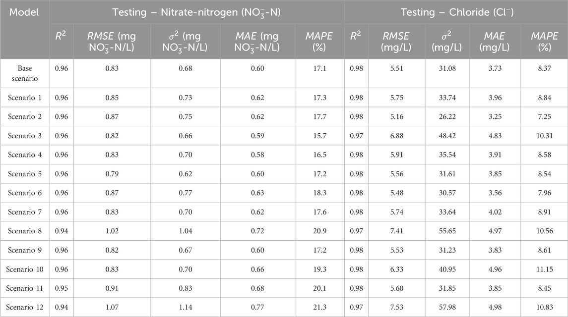
Table 6. Feature importance analysis of the evaluation metrics for the prediction of ${\mathrm{N}\mathrm{O}}_3^{-}$-N and ${\mathrm{C}\mathrm{l}}^{-}$ in surface water for the testing dataset according to the proposed simulation scenarios (Table 3).

Similar results were observed in the training scenarios where the sensitivity of model predictions to the location of sampling sites, hydrological, and field conditions in Scenario #8, 11, and 12 was higher than that of the testing dataset. Although there was no significant change in R² values, that ranged from 0.98 to 0.99, the MAPE values significantly decreased when the previously mentioned input variables were eliminated. The MAPE values were 10.9% for Scenario #8, 13.6% for Scenario #11, and 17.5% for Scenario #12 compared to the base scenario with an MAPE value of 7.8% (Supplementary Table S2). Similarly, the other error metrics of these scenarios were relatively higher than those of the base scenario.

For the prediction of ${\text{Cl}}^{-}$ concentration in surface water, the R² value of the proposed scenarios was not significantly changed compared to the base scenario (R² = 0.98) during the model testing where it ranged from 0.97 to 0.98 (Table 6). However, the MAPE value of Scenarios #3, 8,10, and 12 were slightly increased to be 10.31, 10.56, 11.15, and 10.83%, respectively, compared to the base scenario that had MAPE value of 8.37%. This reflects that the surface water EC, location of the sampling site, water physico-chemical parameters (e.g., surface water temperature), and the field conditions can affect the prediction accuracy of the GPR model in predicting the ${\text{Cl}}^{-}$ concentration in surface water. On the other hand, the MAPE value decreased in Scenarios #2 (7.25%) and 6 (7.96%) when the surface water DO, and average flow rate were excluded from the input variables during the model testing (Table 6).

In the training dataset, the R² was determined to be 0.99 for all the proposed scenarios, including the base scenario, except for Scenario #10 where the R² became 0.98 when the water chemistry and physics parameters were eliminated from the training dataset (Supplementary Table S2). This decrease in R² value was reflected on the error metrics where the MAPE significantly increased from 0.70% for the base scenario to 9.32% for Scenario #10, highlighting the importance of including the physico-chemical water parameters.

4.4 Overall insights about the ML models

4.4.1 Selection of ML regression models

Based on the results of the ML regression model, it was emphasized that the GPR algorithm was the optimal model for predicting the ${\text{NO}}_3^{-}$-N and ${\text{Cl}}^{-}$ concentrations in surface water in the LWC sub-watershed over the observation period. This model resulted in the highest R² value and the least error metrics among the 8 ML regression models employed in the current study. The R² value was 0.99 for predicting the output variables during the model training while it slightly decreased to 0.98 and 0.96 during the model testing of the ${\text{Cl}}^{-}$ and ${\text{NO}}_3^{-}$-N concentrations, respectively. Such high prediction accuracy reflects the robustness of the GPR model in capturing the variations in the output variables over more than 2 years of observations.

In general, the GPR model was the optimal model for predicting the output variables because it is extremely suitable for small and medium-sized datasets (i.e., total number of observations = 161) (Richardson et al., 2017). In addition, GPR is an effective technique for dealing with the model input and output variables with high non-linearity and uncertainty which is common in the nutrient and ${\text{Cl}}^{-}$ transport processes (Elsayed et al., 2024a). GPR techniques also consider the distributions over function instead of a single function, presenting a distribution of likely outcomes rather than predicting a single point estimate (the approach that followed in simple regression models) which can reduce the uncertainty of output variables (Daemi et al., 2019).

Ensemble boosted tree and random forest were the next best models after the GPR model. They yielded relatively high prediction accuracy where the range of R² was 0.98–0.99 for the training dataset and 0.96–0.98 for the testing dataset during the prediction of ${\text{Cl}}^{-}$ and ${\text{NO}}_3^{-}$-N concentrations in surface water. This is mainly because these models can enhance the prediction accuracy by reducing the mis-prediction rates in model variables with the minimal number of iterations (Zhou et al., 2019). They also can develop robust models by avoiding the weak models involved in the ensemble models and increase the contribution of potential candidates for better prediction of the output variables. Moreover, they can capture the complex relationships between the model variables which is common in the nutrient transport applications in surface water. Ultimately, they can effectively deal with noisy datasets with multiple non-linear and uncertain parameters which is appropriate and compatible with the dataset of the LWC sub-watershed (Melesse et al., 2020).

On the other hand, some ML regression models, such as linear regression, were not optimal choices for predicting the output variables using the given input variables. This is mainly because the linear regression model is a simple algorithm to detect the complicated correlations and interdependences between the model variables (Chou et al., 2018). The linear regression model is not suitable for high-dimensional datasets with high uncertainty and non-linearity (Qun’ou et al., 2021). Thus, it is highly recommended to implement more complex models, such as the GPR, ensemble boosted trees, and random forest algorithms, over the linear regression for accurate prediction of ${\text{NO}}_3^{-}$-N and ${\text{Cl}}^{-}$ concentrations in surface water in the LWC sub-watershed. These outcomes are consistent with the major findings of previous ML investigations in a clay agricultural watershed (Elsayed et al., 2023b; Elsayed et al., 2024a), highlighting the complexity of contaminant transport processes in different agricultural settings which requires complex ML algorithms (e.g., ensemble models) than simple models (e.g., linear regression) for better prediction of surface water quality parameters. These models can be employed by stakeholders and decision makers for better quantification of ${\text{Cl}}^{-}$ and ${\text{NO}}_3^{-}$-N levels in the main watercourse within the sub-watershed. Furthermore, additional investigations on different agricultural settings are required to generalize and confirm the applicability of such complex ML models in predicting numerous water quality parameters not only in surface water but also in groundwater and tile drains.

4.4.2 Applicability and transferability of ML models

ML regression models can be used to predict water quality parameters in both surface and groundwater across any agricultural watershed. These output variables may include nitrogen, phosphorus, and ${\text{Cl}}^{-}$ concentrations while incorporating various input variables specific to each watershed, such as hydrological, meteorological, and field conditions. However, the effectiveness and reliability of different ML regression models can vary depending on the environmental characteristics of the watershed. For example, the optimal ML regression models could have strong predictive abilities in other agricultural watersheds with features similar to those of the LWC sub-watershed, such as meteorological conditions (e.g., precipitation), geology (e.g., sandy soils), and geography (e.g., within the Great Lakes Basin). The quality, resolution, and frequency of available datasets also significantly impact the development of reliable and practical models.

Also, diverse monitoring datasets are needed to develop, train, validate, and analyze the ML regression models. These models can potentially be employed by decision makers and stakeholders to assess the risk of nutrient and ${\text{Cl}}^{-}$ transport from agricultural fields to surface water. In addition, these ML models can be used to predict the water quality at unmonitored locations, fill the missing observations of water quality parameters, and identify the governing parameters of the water quality. By monitoring and using the easily observable input variables, such as field conditions, ML models can quantify the contamination levels in surface water. For example, well-trained ML models coupled with continuous monitoring of the physico-chemical water parameters (e.g., temperature and pH) using real-time sensors can assist in obtaining continuous time-series of water quality parameters at the location of these sensors. Accordingly, these models can overcome the challenges of quantifying water quality concentrations using the standard sampling methods, reducing the time, effort, and cost associated with these typical sampling methods.

In this study, a comprehensive dataset with a wide range of variables, including meteorological, hydrological, and field conditions, was used to evaluate the potential of ML regression models in predicting ${\text{NO}}_3^{-}$-N and ${\text{Cl}}^{-}$ concentrations in surface water. Such high-quality, diverse datasets may not be available in other agricultural watersheds. For example, in some watersheds, the number of relevant features may be insufficient for accurate predictions, and the frequency or resolution of data collection may limit the effectiveness of the ML models. These challenges are key limitations in applying ML models as predictive tools for estimating water quality parameters in surface water. Therefore, it is essential to apply these optimal models across various agricultural watersheds, using comprehensive datasets that cover hydrological, meteorological, and field conditions, in order to extend their applicability and overcome the limitations of ML models.

The application of the optimal ML regression models employed in the current study can be extended to include additional datasets from other agricultural watersheds with distinct input and output variables. Moreover, the scope of ML models can be expanded to cover the prediction of groundwater quality parameters. Also, the importance and interpretability analyses can be extended to other datasets that were collected from different agricultural catchments. The proposed ML regression models can be re-trained using new datasets to predict the ${\text{Cl}}^{-}$ and ${\text{NO}}_3^{-}$-N concentrations in surface water, assisting in better understanding of the mechanisms of contaminant transport in surface water. Also, the applicability of these models can be extended to consider additional output variables if these models got exposed to larger dataset with multiple water quality parameters. This should enhance the generalization of the adopted ML regression models to different datasets pertaining to water quality monitoring in surface water.

4.4.3 Major contributions, limitations, and future research steps

In the current study, unlike previous ML studies that focused on a single water quality parameter or a single monitoring site, an integrated multi-site and multi-variable approach was adopted to predict both ${\text{NO}}_3^{-}$-N and ${\text{Cl}}^{-}$ concentrations in surface water across nine distinct observation sites within an agricultural watershed. Such approach enhanced the robustness of the ML models and the corresponding outcomes which can provide a more comprehensive description of the spatial variability of water quality parameters in agricultural watersheds. In addition, our study was capable of bridging the data-driven modeling and water quality interpretation. In other words, while most of regression-based ML studies focus mainly on model performance, our study included conducting a feature importance analysis to identify the most influential factors that can contribute to water quality predictions in surface water. This allowed better understanding of the underlying hydrological and land-use processes driving water quality changes, demonstrating meaningful insights in both ML advancements and practical watershed management. The scope of the current study also covered addressing some challenges associated with agricultural watersheds which are highly dynamic systems influenced by seasonal variability, fertilizer applications, and hydrometeorological conditions. By incorporating a diverse set of input variables (e.g., hydrological and meteorological conditions), the outcomes of this study were more oriented towards investigating the prediction capabilities of regression-based ML models in agricultural watersheds. This can aid in more precise forecasting of water quality parameters in agricultural watersheds, providing critical insights for pollution mitigation and sustainable land management practices.

Although the optimal ML models demonstrated high predictive performance in the Lower Whitemans Creek sub-watershed, their generalization to other watersheds with different hydrological and meteorological conditions remains one of the most critical challenges associated with employing these models in water quality prediction. This is mainly because these ML models are highly dependent on the quality of the training datasets, and their performance may decline when applied to other regions with limited, biased, or inconsistent datasets. Moreover, watersheds with different pollutant transport mechanisms (e.g., wetlands) may require additional and/or different input variables as well as model re-validation and adjustment.

Such limitations create remarkable room for multiple research directions and attempts for further investigation into water quality prediction. For example, future studies can explore the applicability of ML models on a broader range of water quality parameters such as phosphorus concentration in surface water. In addition, the scope of these ML models can be expanded to monitor the water quality parameters in groundwater. Moreover, larger datasets covering multiple hydrological cycles, spatial and seasonal variations should be incorporated to assess model effectiveness over longer observation periods. Also, hybrid modeling approaches that combine ML with process-based hydrological models can offer more interpretable and physically meaningful predictions, bridging the gap between data-driven models and well-established water quality modeling frameworks. Such future research directions formulate more comprehensive assessment of the robustness of ML models in different water quality contexts.

5 Conclusion

In the current study, different groups of ML regression models were systematically employed on a 2-year dataset obtained from a sand plain agricultural sub-watershed in southwestern Ontario, Canada to predict the ${\text{NO}}_3^{-}$-N and ${\text{Cl}}^{-}$ concentrations in surface water in five main channel and four tributary sampling sites using a group of input variables such as hydrological, meteorological, and field conditions. Based on various evaluation metrics, it was demonstrated that the GPR algorithm was the optimal model for predicting the two output variables. The R² value of the GPR model for the ${\text{NO}}_3^{-}$-N concentration in surface water was 0.99 (for training) and 0.96 (for testing) while it was 0.99 (for training) and 0.98 (for testing) for ${\text{Cl}}^{-}$ concentration. In addition, the ensemble bagged tree and random forest models gave high prediction accuracy that was comparable to that obtained by the GPR model especially for the testing datasets. Moreover, a feature importance analysis was conducted to determine the significance of model input variables on the prediction accuracy of the two output variables. Accordingly, it was found that the field conditions, especially the location of sampling sites (main channel and tributary sites), are the governing input variables of accurate prediction of the ${\text{NO}}_3^{-}$-N and ${\text{Cl}}^{-}$ concentrations in surface water. This study provides meaningful insights into the practical benefits of using ML models to complement traditional field monitoring in agricultural watersheds, offering more efficient and precise predictions of water quality parameters in surface water. The major findings of this study underscore that ML regression models can significantly enhance the accuracy and responsiveness of environmental decision-making processes to avoid the deterioration of surface water quality.

Data availability statement

The original contributions presented in the study are included in the article/Supplementary Material, further inquiries can be directed to the corresponding author.

Author contributions

AE: Conceptualization, Data curation, Formal Analysis, Investigation, Methodology, Software, Visualization, Writing–original draft. JL: Conceptualization, Funding acquisition, Project administration, Resources, Supervision, Validation, Writing–review and editing. AB: Conceptualization, Funding acquisition, Project administration, Resources, Supervision, Validation, Writing–review and editing. ML: Funding acquisition, Project administration, Resources, Supervision, Validation, Writing–review and editing, Conceptualization. PG: Funding acquisition, Project administration, Resources, Supervision, Validation, Writing–review and editing, Conceptualization.

Funding

The author(s) declare that financial support was received for the research and/or publication of this article. This work was supported by the Ontario Ministry of the Environment, Conservation and Parks (MECP) and Natural Sciences and Engineering Research Council of Canada (NSERC–Alliance; Grant # 401934).

Acknowledgments

The authors would like to acknowledge Grand River Conservation Authority (GRCA) for access to data and land. The authors would like to thank Floyd Davis for access to the land and support during the field sampling.

Conflict of interest

The authors declare that the research was conducted in the absence of any commercial or financial relationships that could be construed as a potential conflict of interest.

Generative AI statement

The author(s) declare that no Generative AI was used in the creation of this manuscript.

Publisher’s note

All claims expressed in this article are solely those of the authors and do not necessarily represent those of their affiliated organizations, or those of the publisher, the editors and the reviewers. Any product that may be evaluated in this article, or claim that may be made by its manufacturer, is not guaranteed or endorsed by the publisher.

Supplementary material

The Supplementary Material for this article can be found online at: https://www.frontiersin.org/articles/10.3389/fenvs.2025.1543852/full#supplementary-material

References

Aggarwal, C. C. (2016). Data mining: the textbook. Berlin: Springer, 285–426.

Google Scholar

Agriculture and Agri-Food Canada (AAFC) (2023). Annual crop inventory 2022. Available online at: https://open.canada.ca/data/en/dataset/199e4ab6-832b-4434-ac39-e4887d7cc4e5.

Google Scholar

Ahmed, A. N., Othman, F. B., Afan, H. A., Elsha, A., Ming Fai, C., Shabbir Hossain, M., et al. (2019). Machine learning methods for better water quality prediction. J. Hydrology 578, 124084. doi:10.1016/j.jhydrol.2019.124084

CrossRef Full Text | Google Scholar

Ahmed, M. H., and Lin, L. S. (2021). Dissolved oxygen concentration predictions for running waters with different land use land cover using a quantile regression forest machine learning technique. J. Hydrology 597, 126213. doi:10.1016/j.jhydrol.2021.126213

CrossRef Full Text | Google Scholar

Akhtar, N., Izzuddin, M., Ishak, S., Bhawani, S. A., and Umar, K. (2021). Various natural and anthropogenic factors responsible for water quality degradation: a review. Water 13 (19), 2660. doi:10.3390/w13192660

CrossRef Full Text | Google Scholar

Aldrees, A., Hassan, H., Faisal, M., and Mohamed, A. M. (2022). Prediction of water quality indexes with ensemble learners: bagging and boosting. Process Saf. Environ. Prot. 168 (August), 344–361. doi:10.1016/j.psep.2022.10.005

CrossRef Full Text | Google Scholar

Arabgol, R., Sartaj, M., and Asghari, K. (2016). Predicting nitrate concentration and its spatial distribution in groundwater resources using support vector machines (SVMs) model. Environ. Model. Assess. 21 (1), 71–82. doi:10.1007/s10666-015-9468-0

CrossRef Full Text | Google Scholar

Arce-Rodriguez, J. (2024). Nitrate transport in a sand plain aquifer in the Lake Erie Basin. MASc thesis. University of Guelph, 190. Available online at: https://hdl.handle.net/10214/28354.

Google Scholar

Asadollah, S. B. H. S. H., Sharafati, A., Motta, D., and Yaseen, Z. M. (2021). River water quality index prediction and uncertainty analysis: a comparative study of machine learning models. J. Environ. Chem. Eng. 9 (1), 104599. doi:10.1016/j.jece.2020.104599

CrossRef Full Text | Google Scholar

Ashari, A., Paryudi, I., and Tjoa, A. M. (2013). Performance comparison between naïve bayes, decision tree and k-nearest neighbor in searching alternative design in an energy simulation tool. Int. J. Adv. Comput. Sci. Appl. 4 (11), 33–39. doi:10.14569/ijacsa.2013.041105

CrossRef Full Text | Google Scholar

Balson, T., and Ward, A. S. (2022). A machine learning approach to water quality forecasts and sensor network expansion: case study in the Wabash River Basin, United States. Hydrol. Process. 36 (6), 1–15. doi:10.1002/hyp.14619

CrossRef Full Text | Google Scholar

Bedi, S., Samal, A., Ray, C., and Snow, D. (2020). Comparative evaluation of machine learning models for groundwater quality assessment. Environ. Monit. Assess. 192 (12), 776. doi:10.1007/s10661-020-08695-3

PubMed Abstract | CrossRef Full Text | Google Scholar

Behrouz, M. S., Yazdi, M. N., and Sample, D. J. (2022). Using Random Forest, a machine learning approach to predict nitrogen, phosphorus, and sediment event mean concentrations in urban runoff. J. Environ. Manag. 317, 115412. doi:10.1016/j.jenvman.2022.115412

PubMed Abstract | CrossRef Full Text | Google Scholar

Betts, A., Gharabaghi, B., McBean, E. d., Levison, J., and Parker, B. (2015). Salt vulnerability assessment methodology for municipal supply wells. J. Hydrol. 531, 523–533. doi:10.1016/j.jhydrol.2015.11.004

CrossRef Full Text | Google Scholar

Bhattarai, A., Dhakal, S., Gautam, Y., and Bhattarai, R. (2021). Prediction of nitrate and phosphorus concentrations using machine learning algorithms in watersheds with different land use. Water 13 (21), 3096. doi:10.3390/w13213096

CrossRef Full Text | Google Scholar

Canadian Council of Ministers of the Environment (2011). Selected tools to evaluate water monitoring networks for climate change adaptation.

Google Scholar

Canadian Council of Ministers of the Environment (2012). Canadian water quality guidelines for the protection of aquatic life: nitrate. Can. Counc. Minist. Environ. Available online at: http://ceqg-rcqe.ccme.ca/download/en/197.

Google Scholar

Castiblanco, E. S., Groffman, P. M., Duncan, J., Band, L. E., Doheny, E., Emma, T. F., et al. (2023). Long-term trends in nitrate and chloride in streams in an exurban watershed. Urban Ecosyst. 26, 831–844. doi:10.1007/s11252-023-01340-0

CrossRef Full Text | Google Scholar

Cervantes, J., Garcia-Lamont, F., Rodríguez-Mazahua, L., and Lopez, A. (2020). A comprehensive survey on support vector machine classification: applications, challenges and trends. Neurocomputing 408, 189–215. doi:10.1016/j.neucom.2019.10.118

CrossRef Full Text | Google Scholar

Chang, C. F., Garcia, V., Tang, C., Vlahos, P., Wanik, D., Yan, J., et al. (2021). Linking multi-media modeling with machine learning to assess and predict lake chlorophyll a concentrations. J. Gt. Lakes. Res. 47 (6), 1656–1670. doi:10.1016/j.jglr.2021.09.011

PubMed Abstract | CrossRef Full Text | Google Scholar

Chapra, S. C., Dove, A., and Rockwell, D. C. (2009). Great Lakes chloride trends: long-term mass balance and loading analysis. J. Gt. Lakes. Res. 35 (2), 272–284. doi:10.1016/j.jglr.2008.11.013

CrossRef Full Text | Google Scholar

Chou, J., Ho, C., and Hoang, H. (2018). Determining quality of water in reservoir using machine learning. Ecol. Inf. 44, 57–75. doi:10.1016/j.ecoinf.2018.01.005

CrossRef Full Text | Google Scholar

Chow, R., Scheidegger, R., Doppler, T., Dietzel, A., Fenicia, F., and Stamm, C. (2020). A review of long-term pesticide monitoring studies to assess surface water quality trends. Water Res. X 9, 100064. doi:10.1016/j.wroa.2020.100064

PubMed Abstract | CrossRef Full Text | Google Scholar

Daemi, A., Kodamana, H., and Huang, B. (2019). Gaussian process modelling with Gaussian mixture likelihood. J. Process Control 81, 209–220. doi:10.1016/j.jprocont.2019.06.007

CrossRef Full Text | Google Scholar

David, M. B., Mitchell, C. A., Gentry, L. E., and Salemme, R. K. (2016). Chloride sources and losses in two tile-drained agricultural watersheds. J. Environ. Qual. 45, 341–348. doi:10.2134/jeq2015.06.0302

PubMed Abstract | CrossRef Full Text | Google Scholar

D’Haene, K., Waele, J. D., Neve, S. D., and Hofman, G. (2022). Agriculture, Ecosystems and Environment Spatial distribution of the relationship between nitrate residues in soil and surface water quality revealed through attenuation factors. Agric. Ecosyst. Environ. 330 (January), 107889. doi:10.1016/j.agee.2022.107889

CrossRef Full Text | Google Scholar

El Bilali, A., and Taleb, A. (2020). Prediction of irrigation water quality parameters using machine learning models in a semi-arid environment. J. Saudi Soc. Agric. Sci. 19 (7), 439–451. doi:10.1016/j.jssas.2020.08.001

CrossRef Full Text | Google Scholar

Elsayed, A., Ghaith, M., Yosri, A., Li, Z., and El-Dakhakhni, W. (2024b). Genetic programming expressions for effluent quality prediction: towards AI-driven monitoring and management of wastewater treatment plants. J. Environ. Manag. 356 (October 2023), 120510. doi:10.1016/j.jenvman.2024.120510

PubMed Abstract | CrossRef Full Text | Google Scholar

Elsayed, A., Hurdle, M., and Kim, Y. (2021). Comprehensive model applications for better understanding of pilot-scale membrane-aerated biofilm reactor performance. J. Water Process Eng. 40, 101894. doi:10.1016/j.jwpe.2020.101894

CrossRef Full Text | Google Scholar

Elsayed, A., Rixon, S., Levison, J., Binns, A., and Goel, P. (2023b). Application of classification machine learning algorithms for characterizing nutrient transport in a clay plain agricultural watershed. J. Environ. Manage. 345, 118924. doi:10.1016/j.jenvman.2023.118924

PubMed Abstract | CrossRef Full Text | Google Scholar

Elsayed, A., Rixon, S., Levison, J., Binns, A., and Goel, P. (2024a). Machine learning models for prediction of nutrient concentrations in surface water in an agricultural watershed. J. Environ. Manag. 372, 123305. doi:10.1016/j.jenvman.2024.123305

PubMed Abstract | CrossRef Full Text | Google Scholar

Elsayed, A., Rixon, S., Zeuner, C., Levison, J., Binns, A., and Goel, P. (2023a). Text mining-aided meta-research on nutrient dynamics in surface water and groundwater: popular topics and perceived gaps. J. Hydrology 626 (PB), 130338. doi:10.1016/j.jhydrol.2023.130338

CrossRef Full Text | Google Scholar

Elsayed, A., Siam, A., and El-Dakhakhni, W. (2022b). Machine learning classification algorithms for inadequate wastewater treatment risk mitigation. Process Saf. Environ. Prot. 159, 1224–1235. doi:10.1016/j.psep.2022.01.065

CrossRef Full Text | Google Scholar

Elsayed, A., Yu, J., Lee, T., and Kim, Y. (2022a). Model study on real-time aeration based on nitrite for effective operation of single-stage anammox. Environ. Res. 212, 113554. doi:10.1016/j.envres.2022.113554

PubMed Abstract | CrossRef Full Text | Google Scholar

Environment and Climate Change Canada (2021). Canada-US Great Lakes water quality agreement. Government of Canada. Available online at: https://www.canada.ca/en/environment-climate-change/services/great-lakes-protection/canada-united-states-water-quality-agreement.html.

Google Scholar

Environment and Climate Change Canada (ECCC) (2017). Phosphorus and excess algal growth.

Google Scholar

Evans, J. D. (1996). Straightforward statistics for the behavioral sciences. Pacific Grove: Thomson Brooks/Cole Publishing Co.

Google Scholar

Farazan, S. Z., Paudyal, D., Chadalavada, S., and Alam, M. J. (2024). Temporal dynamics and predictive modelling of streamflow and water quality using advanced statistical and ensemble machine learning techniques. Water 16 (15), 2107. doi:10.3390/w16152107

CrossRef Full Text | Google Scholar

Gardner, S. G., Levison, J., Parker, B. L., and Martin, R. C. (2020). Groundwater nitrate in three distinct hydrogeologic and land-use settings in southwestern Ontario, Canada. Hydrogeology J. 28, 1891–1908. doi:10.1007/s10040-020-02156-4

CrossRef Full Text | Google Scholar

Gianfagna, C. C., Johnson, C. E., Chandler, D. G., and Hofmann, C. (2015). Watershed area ratio accurately predicts daily streamflow in nested catchments in the Catskills, New York. J. Hydrology Regional Stud. 4, 583–594. doi:10.1016/j.ejrh.2015.09.002

CrossRef Full Text | Google Scholar

Gondia, A., Ezzeldin, M., and El-dakhakhni, W. (2022). Machine learning – based decision support framework for construction injury severity prediction and risk mitigation. ASCE-ASME J. Risk Uncertain. Eng. Syst. Part A Civ. Eng. 8 (3), 1–17. doi:10.1061/AJRUA6.0001239

CrossRef Full Text | Google Scholar

Gorgoglione, A., Castro, A., Iacobellis, V., and Gioia, A. (2021). A comparison of linear and non-linear machine learning techniques (PCA and SOM) for characterizing urban nutrient runoff. Sustainability 13 (4), 2054–2119. doi:10.3390/su13042054

CrossRef Full Text | Google Scholar

Granato, G. E., DeSimone, L. A., Barbaro, J. R., and Jeznach, L. C. (2015). Methods for evaluating potential sources of chloride in surface waters and groundwaters of the conterminous United States. US Geological Survey.

CrossRef Full Text | Google Scholar

Ha, N. T., Nguyen, H. Q., Truong, N. C. Q., Le, T. L., Thai, V. N., and Pham, T. L. (2020). Estimation of nitrogen and phosphorus concentrations from water quality surrogates using machine learning in the Tri an Reservoir, Vietnam. Environ. Monit. Assess. 192 (12), 789. doi:10.1007/s10661-020-08731-2

PubMed Abstract | CrossRef Full Text | Google Scholar

Hafeez, S., Wong, M. S., Ho, H. C., Nazeer, M., Nichol, J., Abbas, S., et al. (2019). Comparison of machine learning algorithms for retrieval of water quality indicators in case-II waters: a case study of Hong Kong. Remote Sens. 11, 617. doi:10.3390/rs11060617

CrossRef Full Text | Google Scholar

Harrison, J. W., Lucius, M. A., Farrell, J. L., Eichler, L. W., and Relyea, R. A. (2021). Prediction of stream nitrogen and phosphorus concentrations from high-frequency sensors using Random Forests Regression. Sci. Total Environ. 763, 143005. doi:10.1016/j.scitotenv.2020.143005

PubMed Abstract | CrossRef Full Text | Google Scholar

Health Canada (1987). Guidelines for Canadian drinking water quality: guideline technical document. Chloride.

Google Scholar

Health Canada (1999). Guidelines for Canadian drinking water quality: guideline technical document. Chloride.

Google Scholar

Imani, M., Hasan, M. M., Bittencourt, L. F., McClymont, K., and Kapelan, Z. (2021). A novel machine learning application: water quality resilience prediction Model. Sci. Total Environ. 768, 144459. doi:10.1016/j.scitotenv.2020.144459

PubMed Abstract | CrossRef Full Text | Google Scholar

Islam, A. R. M. T., Chandra, S., Chowdhuri, I., Salam, R., Islam, S., Zahid, A., et al. (2021). Application of novel framework approach for prediction of nitrate concentration susceptibility in coastal multi-aquifers, Bangladesh. Sci. Total Environ. 801, 149811. doi:10.1016/j.scitotenv.2021.149811

PubMed Abstract | CrossRef Full Text | Google Scholar

Jung, C., Ahn, S., Sheng, Z., Ayana, E. K., Srinivasan, R., and Yeganantham, D. (2021). Evaluate river water salinity in a semi-arid agricultural watershed by coupling ensemble machine learning technique with SWAT model. J. Am. Water Resour. Assoc. 58, 1175–1188. doi:10.1111/1752-1688.12958

CrossRef Full Text | Google Scholar

Kaushal, S. S., Groffman, P. M., Likens, G. E., Belt, K. T., Stack, W. P., Kelly, V. R., et al. (2005). Increased salinization of fresh water in the northeastern United States. Proc. Natl. Acad. Sci. U.S.A. 102, 13517–13520. doi:10.1073/pnas.0506414102

PubMed Abstract | CrossRef Full Text | Google Scholar

Khoi, D. N., Quan, N. T., Linh, D. Q., Nhi, P. T. T., and Thuy, N. T. D. (2022). Using machine learning models for predicting the water quality index in the La buong river, vietnam. Water 14, 1552–1612. doi:10.3390/w14101552

CrossRef Full Text | Google Scholar

Kim, T., Yang, T., Gao, S., Zhang, L., Ding, Z., Wen, X., et al. (2021). Can artificial intelligence and data-driven machine learning models match or even replace process-driven hydrologic models for streamflow simulation?a case study of four watersheds with different hydro-climatic regions across the CONUS. J. Hydrology 598, 126423. doi:10.1016/j.jhydrol.2021.126423

CrossRef Full Text | Google Scholar

Knoll, L., Breuer, L., and Bach, M. (2019). Large scale prediction of groundwater nitrate concentrations from spatial data using machine learning. Sci. Total Environ. 668, 1317–1327. doi:10.1016/j.scitotenv.2019.03.045

PubMed Abstract | CrossRef Full Text | Google Scholar

Kouadri, S., Elbeltagi, A., Reza, A., Islam, T., and Kateb, S. (2021). Performance of machine learning methods in predicting water quality index based on irregular data set: application on Illizi region (Algerian southeast). Appl. Water Sci. 11 (12), 190–220. doi:10.1007/s13201-021-01528-9

CrossRef Full Text | Google Scholar

Kovacs, D. J., Li, Z., Baetz, B. W., Hong, Y., Donnaz, S., Zhao, X., et al. (2022). Membrane fouling prediction and uncertainty analysis using machine learning: a wastewater treatment plant case study. J. Membr. Sci. 660, 120817. doi:10.1016/j.memsci.2022.120817

CrossRef Full Text | Google Scholar

Kuzmanovski, V., Trajanov, A., Leprince, F., Džeroski, S., and Debeljak, M. (2015). Modeling water outflow from tile-drained agricultural fields. Sci. Total Environ. 505, 390–401. doi:10.1016/j.scitotenv.2014.10.009

PubMed Abstract | CrossRef Full Text | Google Scholar

Larocque, M., Levison, J., Gagné, S., and Saleem, S. (2019). “Groundwater use for agricultural production – current water budget and expected trends under climate change,” in Final report submitted to MAPAQ and OMAFRA. Université du Québec à Montréal and University of Guelph. Montréal (Québec) and Guelph (Ontario), 67.

Google Scholar

Lax, S., Peterson, E., and Van der Hoven, S. (2017). Stream chloride concentrations as a function of land use: a comparison of an agricultural watershed to an urban agricultural watershed. Environ. Earth Sci. 76 (20), 708–712. doi:10.1007/s12665-017-7059-x

CrossRef Full Text | Google Scholar

Li, X., Li, Z., Huang, W., and Zhou, P. (2020). Performance of statistical and machine learning ensembles for daily temperature downscaling. Theor. Appl. Climatol. 140, 571–588. doi:10.1007/s00704-020-03098-3

CrossRef Full Text | Google Scholar

Liang, K., Jiang, Y., Qi, J., Fuller, K., Nyiraneza, J., and Meng, F. R. (2020). Characterizing the impacts of land use on nitrate load and water yield in an agricultural watershed in Atlantic Canada. Sci. Total Environ. 729, 138793. doi:10.1016/j.scitotenv.2020.138793

PubMed Abstract | CrossRef Full Text | Google Scholar

Mackie, C., Lackey, R., Levison, J., and Rodrigues, L. (2022). Groundwater as a source and pathway for road salt contamination of surface water in the Lake Ontario Basin: a review. J. Gt. Lakes. Res. 48 (1), 24–36. doi:10.1016/j.jglr.2021.11.015

CrossRef Full Text | Google Scholar

Mackie, C., Levison, J., Binns, A., and O’Halloran, I. (2021). Groundwater-surface water interactions and agricultural nutrient transport in a Great Lakes clay plain system. J. Gt. Lakes. Res. 47 (1), 145–159. doi:10.1016/j.jglr.2020.11.008

CrossRef Full Text | Google Scholar

Marshall, R., Levison, J., Parker, B., and Mcbean, E. (2022). Septic system impacts on source water: two novel field tracer experiments in fractured sedimentary bedrock. Sustainability 14, 1959. doi:10.3390/su14041959

CrossRef Full Text | Google Scholar

May, H., Rixon, S., Gardner, S., Goel, P., Levison, J., and Binns, A. (2023). Investigating relationships between climate controls and nutrient flux in surface waters, sediments, and subsurface pathways in an agricultural clay catchment of the Great Lakes Basin. Sci. Total Environ. 864, 160979. doi:10.1016/j.scitotenv.2022.160979

PubMed Abstract | CrossRef Full Text | Google Scholar

Melesse, A. M., Khosravi, K., Tiefenbacher, J. P., Heddam, S., Kim, S., Mosavi, A., et al. (2020). River water salinity prediction using hybrid machine learning models. Water 12 (10), 2951–3021. doi:10.3390/w12102951

CrossRef Full Text | Google Scholar

Merchán, D., Casalí, J., Valle, J. D., Lersundi, D., Campo-bescós, M. A., Giménez, R., et al. (2018). Runoff, nutrients, sediment and salt yields in an irrigated watershed in southern Navarre (Spain). Agric. Water Manag. 195, 120–132. doi:10.1016/j.agwat.2017.10.004

CrossRef Full Text | Google Scholar

Messier, K. P., Wheeler, D. C., Flory, A. R., Jones, R. R., Patel, D., Nolan, B. T., et al. (2019). Modeling groundwater nitrate exposure in private wells of North Carolina for the Agricultural Health Study. Sci. Total Environ. 655, 512–519. doi:10.1016/j.scitotenv.2018.11.022

PubMed Abstract | CrossRef Full Text | Google Scholar

Miller, M. P., Tesoriero, A. J., Capel, P. D., Pellerin, B. A., Hyer, K. E., Burns, D. A., et al. (2015). Quantifying watershed-scale groundwater loading and in-stream fate of nitrate using high-frequency water quality data. Water Resour. Res. 52, 330–347. doi:10.1002/2015WR017753

CrossRef Full Text | Google Scholar

Ministry of the Environment, Conservation and Parks (2021). Canada-ontario Great lakes agreement. Government of Ontario. Available online at: https://www.ontario.ca/document/canada-ontario-great-lakes-agreement.

Google Scholar

Mosavi, A., Hosseini, F. S., Choubin, B., Goodarzi, M., Dineva, A. A., and Sardooi, E. R. (2021). Ensemble boosting and bagging based machine learning models for groundwater potential prediction. Water Resour. Manag. 35 (1), 23–37. doi:10.1007/s11269-020-02704-3

CrossRef Full Text | Google Scholar

Mukaka, M. M. (2012). A guide to appropriate use of correlation coefficient in medical research. Malawi Med. J. 24 (3), 69e71.

Google Scholar

Mullaney, J. R., Lorenz, D. L., and Arnston, A. D. (2009). Chloride in groundwater and surface water in areas underlain by the glacial aquifer system, northern United States. Reston, VA: US Geological Survey.

Google Scholar

Najah Ahmed, A., Binti Othman, F., Abdulmohsin Afan, H., Khaleel Ibrahim, R., Ming Fai, C., Shabbir Hossain, M., et al. (2019). Machine learning methods for better water quality prediction. J. Hydrology 578, 124084. doi:10.1016/j.jhydrol.2019.124084

CrossRef Full Text | Google Scholar

Osman, A. R. M. (2017). Water use conflict: a characterization and water quantity study in an agriculturally stressed sub-catchment in Southern Ontario. MASc thesis, Univ. Guelph, 190. Available online at: http://hdl.handle.net/10214/12134.

Google Scholar

Oswald, C. J., Giberson, G., Nicholls, E., Wellen, C., and Oni, S. (2019). Spatial distribution and extent of urban land cover control watershed-scale chloride retention. Sci. Total Environ. 652, 278–288. doi:10.1016/j.scitotenv.2018.10.242

PubMed Abstract | CrossRef Full Text | Google Scholar

Overbo, A., Heger, S., and Gulliver, J. (2021). Evaluation of chloride contributions from major point and nonpoint sources in a northern U.S. state. Sci. Total Environ. 764, 144179–179. doi:10.1016/j.scitotenv.2020.144179

PubMed Abstract | CrossRef Full Text | Google Scholar

Pandey, P., Gupta, A. P., Dutta, J., and Thakur, T. K. (2023). “Role of artificial intelligence in water conservation with special reference to India,” in Emerging technologies for water supply, conservation and management. Editors E. Balaji, G. Veeraswamy, P. Mannala, and S. Madhav (Cham, Switzerland: Springer). doi:10.1007/978-3-031-35279-9_4

CrossRef Full Text | Google Scholar

Park, Y., Kim, Y., Park, S., Shin, W., and Lee, K. (2018). Water quality impacts of irrigation return flow on stream and groundwater in an intensive agricultural watershed. Sci. Total Environ. 630, 859–868. doi:10.1016/j.scitotenv.2018.02.113

PubMed Abstract | CrossRef Full Text | Google Scholar

Perera, N., Gharabaghi, B., and Howard, K. (2013). Groundwater chloride response in the Highland Creek watershed due to road salt application: a re-assessment after 20 years. J. Hydrol. 479, 159–168. doi:10.1016/j.jhydrol.2012.11.057

CrossRef Full Text | Google Scholar

Perović, M., Šenk, I., Tarjan, L., Obradović, V., and Dimkić, M. (2021). Machine learning models for predicting the ammonium concentration in alluvial groundwaters. Environ. Model. Assess. 1, 1–17. doi:10.1007/s10666-020-09731-9

CrossRef Full Text | Google Scholar

Persaud, E., Levison, J., Ali, G., and Robinson, C. (2023). Using isotopic tracers to enhance routine watershed monitoring – insights from an intensively managed agricultural catchment. J. Environ. Manag. 344, 118364. doi:10.1016/j.jenvman.2023.118364

PubMed Abstract | CrossRef Full Text | Google Scholar

Portuguez-maurtua, M., Arumi, J. L., Lagos, O., Stehr, A., and Arquiñigo, N. M. (2022). Filling gaps in daily precipitation series using regression and machine learning in inter-andean watersheds. Water 14 (11), 1799. doi:10.3390/w14111799

CrossRef Full Text | Google Scholar

Qiao, Z., Sun, S., Jiang, Q., Xiao, L., Wang, Y., and Yan, H. (2021). Retrieval of total phosphorus concentration in the surface water of miyun reservoir based on remote sensing data and machine learning algorithms. Remote Sens. 13 (22), 4662. doi:10.3390/rs13224662

CrossRef Full Text | Google Scholar

Qun’ou, J., Lidan, X., Siyang, S., Meilin, W., and Huijie, X. (2021). Retrieval model for total nitrogen concentration based on UAV hyper spectral remote sensing data and machine learning algorithms – a case study in the Miyun Reservoir, China. Ecol. Indic. 124, 107356. doi:10.1016/j.ecolind.2021.107356

CrossRef Full Text | Google Scholar

Richards, G., Gilmore, T. E., Mittelstet, A. R., Messer, T. L., and Snow, D. D. (2021). Baseflow nitrate dynamics within nested watersheds of an agricultural stream in Nebraska, USA. Agric. Ecosyst. Environ. 308 (June 2020), 107223. doi:10.1016/j.agee.2020.107223

CrossRef Full Text | Google Scholar

Richardson, R. R., Osborne, M. A., and Howey, D. A. (2017). Gaussian process regression for forecasting battery state of health. J. Power Sources 357, 209–219. doi:10.1016/j.jpowsour.2017.05.004

CrossRef Full Text | Google Scholar

Rixon, S., Levison, J., Binns, A., and Persaud, E. (2020). Spatiotemporal variations of nitrogen and phosphorus in a clay plain hydrological system in the Great Lakes Basin. Sci. Total Environ. 714, 136328. doi:10.1016/j.scitotenv.2019.136328

PubMed Abstract | CrossRef Full Text | Google Scholar

Rixon, S., May, H., Persaud, E., Elsayed, A., Levison, J., Binns, A., et al. (2024). Subsurface influences on watershed nutrient concentrations and loading in a clay dominated agricultural system. J. Hydrology 645, 132140. doi:10.1016/j.jhydrol.2024.132140

CrossRef Full Text | Google Scholar

Sajib, A. M., Diganta, M. T. M., Moniruzzaman, M., Rahman, A., Dabrowski, A. I., Uddin, M. G., et al. (2024). Assessing water quality of an ecologically critical urban canal incorporating machine learning approaches. Ecol. Inf. 80, 102514. doi:10.1016/j.ecoinf.2024.102514

CrossRef Full Text | Google Scholar

Sajib, A. M., Diganta, M. T. M., Rahman, A., Dabrowski, T., Olbert, A. I., and Uddin, M. G. (2023). Developing a novel tool for assessing the groundwater incorporating water quality index and machine learning approach. Groundw. Sustain. Dev. 23, 101049. doi:10.1016/j.gsd.2023.101049

CrossRef Full Text | Google Scholar

Sakizadeh, M., Zhang, C., and Milewski, A. (2024). Spatial distribution pattern and health risk of groundwater contamination by cadmium, manganese, lead and nitrate in groundwater of an arid area. Environ. Geochem. Health 46 (3), 80–25. doi:10.1007/s10653-023-01845-9

PubMed Abstract | CrossRef Full Text | Google Scholar

Shah, M. I., Alaloul, W. S., Alqahtani, A., Aldrees, A., Musarat, M. A., and Javed, M. F. (2021). Predictive modeling approach for surface water quality: development and comparison of machine learning models. Sustainability 13, 7515. doi:10.3390/su13147515

CrossRef Full Text | Google Scholar

Sigler, W. A., Ewing, S. A., Jones, C. A., Payn, R. A., Brookshire, E. N. J., Klassen, J. K., et al. (2018). Connections among soil, ground, and surface water chemistries characterize nitrogen loss from an agricultural landscape in the upper Missouri River Basin. J. Hydrology 556, 247–261. doi:10.1016/j.jhydrol.2017.10.018

CrossRef Full Text | Google Scholar

Singh, B., and Craswell, E. (2021). Fertilizers and nitrate pollution of surface and ground water: an increasingly pervasive global problem. SN Appl. Sci. 3 (4), 1–24. doi:10.1007/s42452-021-04521-8

CrossRef Full Text | Google Scholar

Sorichetti, R. J., Raby, M., Holeton, C., Benoit, N., Carson, L., Desellas, A., et al. (2022). Chloride trends in Ontario ’ s surface and groundwaters. J. Gt. Lakes. 48, 512–525. doi:10.1016/j.jglr.2022.01.015

CrossRef Full Text | Google Scholar

Steele, M. K., and Aitkenhead-Peteerson, R. (2011). Long-term sodium and chloride surface water exports from the Dallas/Fort Worth region. Sci. Total Environ. 409 (16), 3021–3032. doi:10.1016/j.scitotenv.2011.04.015

PubMed Abstract | CrossRef Full Text | Google Scholar

Steele, R., and Veliz, M. (2007). Water quality in the ausable bayfield maitland valley. Retrievedfrom. Available online at: http://www.sourcewaterinfo.on.ca/images/uploaded/uploadedDownloads/WC_Chap2_Mar_08.pdf.

Google Scholar

Stelzer, R. S., and Scott, J. T. (2018). Predicting nitrate retention at the groundwater-surface water interface in sandplain streams. J. Geophys. Res. Biogeosciences 123 (9), 2824–2838. doi:10.1029/2018JG004423

CrossRef Full Text | Google Scholar

Stets, E. G., Lee, C. J., Lytle, D. A., and Schock, M. R. (2018). Increasing chloride in rivers of the conterminous U . S. and linkages to potential corrosivity and lead action level exceedances in drinking water. Sci. Total Environ. 613–614, 1498–1509. doi:10.1016/j.scitotenv.2017.07.119

PubMed Abstract | CrossRef Full Text | Google Scholar

Subbarayan, S., Thiyagarajan, S., Karuppannan, S., and Panneerselvam, B. (2024). Enhancing groundwater vulnerability assessment: comparative study of three machine learning models and five classification schemes for Cuddalore district. Environ. Res. 242 (July 2023), 117769. doi:10.1016/j.envres.2023.117769

PubMed Abstract | CrossRef Full Text | Google Scholar

Syeed, M. M. M., Hossain, S., Karim, R., Faisal, M., Hasan, M., and Hayat, R. (2023). Surface water quality profiling using the water quality index, pollution index and statistical methods: a critical review. Environ. Sustain. Indic. 18 (January), 100247. doi:10.1016/j.indic.2023.100247

CrossRef Full Text | Google Scholar

Tian, S., Youssef, M. A., Richards, R. P., Liu, J., Baker, D. B., and Liu, Y. (2016). Different seasonality of nitrate export from an agricultural watershed and an urbanized watershed in Midwestern USA. J. Hydrology 541, 1375–1384. doi:10.1016/j.jhydrol.2016.08.042

CrossRef Full Text | Google Scholar

Uddin, G., Nash, S., Rahman, A., Dabrowski, T., and Olbert, A. I. (2024). Data-driven modelling for assessing trophic status in marine ecosystems using machine learning approaches. Environ. Res. 242 (July 2023), 117755. doi:10.1016/j.envres.2023.117755

PubMed Abstract | CrossRef Full Text | Google Scholar

Varadharajan, C., Appling, A. P., Arora, B., Christianson, D. S., Hendrix, V. C., Kumar, V., et al. (2022). Can machine learning accelerate process understanding and decision relevant predictions of river water quality? Hydrol. Process. 36 (4), 1–22. doi:10.1002/hyp.14565

CrossRef Full Text | Google Scholar

Wagh, V., Panaskar, D., Muley, A., Mukate, S., and Gaikwad, S. (2018). Neural network modelling for nitrate concentration in groundwater of Kadava River basin, Nashik, Maharashtra, India. Groundw. Sustain. Dev. 7, 436–445. doi:10.1016/j.gsd.2017.12.012

CrossRef Full Text | Google Scholar

Wang, R., Kim, J. H., and Li, M. H. (2021). Predicting stream water quality under different urban development pattern scenarios with an interpretable machine learning approach. Sci. Total Environ. 761, 144057. doi:10.1016/j.scitotenv.2020.144057

PubMed Abstract | CrossRef Full Text | Google Scholar

Wang, S., Wang, Y., Wang, Y., and Wang, Z. (2022a). Assessment of influencing factors on non-point source pollution critical source areas in an agricultural watershed. Ecol. Indic. 141 (35), 109084. doi:10.1016/j.ecolind.2022.109084

CrossRef Full Text | Google Scholar

Wang, X., Xu, Y. J., and Zhang, L. (2022b). Watershed scale spatiotemporal nitrogen transport and source tracing using dual isotopes among surface water, sediments and groundwater in the Yiluo River Watershed, Middle of China. Sci. Total Environ. 833 (March), 155180. doi:10.1016/j.scitotenv.2022.155180

PubMed Abstract | CrossRef Full Text | Google Scholar

Wells, M. J., Gilmore, T. E., Nelson, N., Mittelstet, A., and Böhlke, J. K. (2021). Determination of vadose zone and saturated zone nitrate lag times using long-Term groundwater monitoring data and statistical machine learning. Hydrology Earth Syst. Sci. 25 (2), 811–829. doi:10.5194/hess-25-811-2021

CrossRef Full Text | Google Scholar

Wheeler, D. C., Nolan, B. T., Flory, A. R., Dellavalle, C. T., and Ward, M. H. (2015). Modeling groundwater nitrate concentrations in private wells in Iowa. Sci. Total Environ. 536, 481–488. doi:10.1016/j.scitotenv.2015.07.080

PubMed Abstract | CrossRef Full Text | Google Scholar

Wong, A. (2011). Water use inventory report for the Grand River watershed. GRCA.

Google Scholar

Xu, T., Coco, G., and Neale, M. (2020). A predictive model of recreational water quality based on adaptive synthetic sampling algorithms and machine learning. Water Res. 177, 115788. doi:10.1016/j.watres.2020.115788

PubMed Abstract | CrossRef Full Text | Google Scholar

Yang, Y., Shang, X., Chen, Z., Mei, K., Wang, Z., Dahlgren, R. A., et al. (2021). A support vector regression model to predict nitrate-nitrogen isotopic composition using hydro-chemical variables. J. Environ. Manag. 290 (November 2020), 112674. doi:10.1016/j.jenvman.2021.112674

PubMed Abstract | CrossRef Full Text | Google Scholar

Yang, Y., Yuan, Y., Xiong, G., Yin, Z., Guo, Y., Song, J., et al. (2024). Patterns of nitrate load variability under surface water-groundwater interactions in agriculturally intensive valley watersheds. Water Res. 267 (August), 122474. doi:10.1016/j.watres.2024.122474

PubMed Abstract | CrossRef Full Text | Google Scholar

Yu, J., Tian, Y., Wang, X., and Zheng, C. (2021). Using machine learning to reveal spatiotemporal complexity and driving forces of water quality changes in Hong Kong marine water. J. Hydrology 603, 126841. doi:10.1016/j.jhydrol.2021.126841

CrossRef Full Text | Google Scholar

Zeuner, C., Levison, J., and Larocque, M. (2025). Insights on nitrate transport in a shallow, sandy aquifer at various temporal and spatial scales. Front. Environ. Sci.

Google Scholar

Zhang, Z., Huang, J., Duan, S., Huang, Y., Cai, J., and Bian, J. (2022). Use of interpretable machine learning to identify the factors influencing the nonlinear linkage between land use and river water quality in the Chesapeake Bay watershed. Ecol. Indic. 140, 108977. doi:10.1016/j.ecolind.2022.108977

CrossRef Full Text | Google Scholar

Zheng, Y., Wei, J., Zhang, W., Zhang, Y., Zhang, T., and Zhou, Y. (2024). An ensemble model for accurate prediction of key water quality parameters in river based on deep learning methods. J. Environ. Manag. 366 (July), 121932. doi:10.1016/j.jenvman.2024.121932

PubMed Abstract | CrossRef Full Text | Google Scholar

Zhou, P., Li, Z., Snowling, S., Baetz, B. W., Na, D., and Boyd, G. (2019). A random forest model for inflow prediction at wastewater treatment plants. Stoch. Environ. Res. Risk Assess. 33 (10), 1781–1792. doi:10.1007/s00477-019-01732-9

CrossRef Full Text | Google Scholar