- 1Department of Geographic Science and Tourism, Jilin Normal University, Siping, China
- 2Department of Geo-Exploration Science and Technology, Jilin University, Changchun, China
Introduction: Forest fires, grassland fires, heap coking, straw burning, and volcanic eruptions are thermal anomalies. They attract attention and are designated as high-temperature targets. They can be retrieved macroscopically and quickly by remote sensing technology.
Methods: In temperature inversion, the mid-infrared (MIR, 3∼5 μm) and thermal infrared (TIR, 8∼14 μm) band data are most commonly used for temperature inversion. However, it is difficult to effectively retrieve the temperature of small-area high-temperature targets with them; the SWIR band data can perform this task more effectively. Additionally, inversion methods for short-wave infrared (SWIR, 1.3∼2.5 μm) and TIR band data are different. These differences lie in the mechanisms and models. Therefore, we use SWIR and TIR band data to retrieve heap coking temperature with Landsat 7 and Landsat 8 data.
Results: SWIR data obtained the results 496∼651 K and 912 K, and TIR data obtained the results 313∼334 K and 320 K.
Conclusion: The SWIR inversion results have higher accuracy than the TIR inversion results. The inversion results are closer to the actual temperature of local coking. For this reason, SWIR is more suitable for temperature inversion of small-area high-temperature targets.
1 Introduction
On Earth, the temperatures of high-temperature targets [forest fires (Adab et al., 2013; Di Biase and Laneve, 2018; Lim et al., 2019; Hashimoto et al., 2021), grassland fires, heap coking (Kong et al., 2005; Biswal and Gorai, 2020), straw burning, volcanic eruptions (Wright et al., 1999), etc.] are significantly higher than those of other normal-temperature objects. Using remote sensing technology to perform temperature inversion (Ermida et al., 2020) has the advantages of low cost and high efficiency. Land surface temperature inversion primarily utilizes TIR or MIR band data (Giglio et al., 2000). Existing methods generally assume that the components and temperatures within the pixels are uniform (Schroeder et al., 2014a; Schroeder et al., 2014b). In addition, emitted radiation is the only aspect that needs to be considered. These algorithms include single window and split window. They are applied in land surface temperature inversion (Yu, 2014; Yu, 2017; Stefanidou et al., 2019; Laneve et al., 2020; Santana et al., 2020; Ehsani et al., 2020), resource investigation (Laneve et al., 2019; Shan et al., 2020; Xu et al., 2021), and environmental monitoring (Veraverbeke et al., 2014; Xu and Zhong, 2017; Szpakowski and Jensen, 2019; Yin et al., 2020). MIR and TIR remote sensing data are heavily affected by atmospheric background radiation. The limitation in spatial resolution is another important effect. These factors make it difficult to effectively retrieve the temperature of small-area high-temperature targets. It is difficult to differentiate high-temperature targets from the background of the normal-temperature objects (Pan et al., 2009; Yu et al., 2016).
According to the law of black-body radiation, in the SWIR band, the radiation from normal-temperature objects (temperature 300 K±) is primarily the reflected energy of solar radiation (Yu et al., 2014a; Yu et al., 2014b). For high-temperature targets, the energy contains not only reflected radiation but also its own emitted radiation. When the temperature reaches a certain level (temperature 500 K ± or higher), the emitted radiation energy will be close to or even exceed the reflected radiation energy of normal-temperature objects. In the instantaneous field of view (IFOV) of remote sensor detection, there are both normal-temperature objects and high-temperature targets. The energy corresponding to the DN value of the mixed pixel is composed of the reflected energy of normal-temperature objects and the emitted energy of high-temperature targets. This spectral feature is significantly different from that of a pure pixel of a normal-temperature object. In the mixed pixel, if the emission energy of the high-temperature target can be separated from the mixed energy, the temperature and area (sub-pixel area) of the high-temperature target can be determined using the black-body radiation law (Planck function) (Pan et al., 2009; Yu et al., 2016). TIR temperature inversion only considers emitted energy (Guo et al., 2020; Maithani et al., 2022; Sekertekin and Bonafoni, 2020a; Sekertekin and Bonafoni, 2020b; Yu, 2014). Moreover, the temperature inversion mechanisms of SWIR and TIR bands are very different. We can derive a physical model from the law mentioned above. Through the physical model, we understand that SWIR is more sensitive for research on high-temperature targets than TIR. Therefore, this paper will use SWIR and TIR data (Barducci et al., 2004; Dennison and Matheson, 2011) to compare the temperature inversion of high-temperature targets. The study areas are in Shanxi Province and Liaoning Province, where we have conducted field verification (Yu et al., 2016; Yu, 2017).
2 Methodology
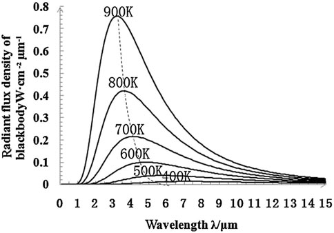
Any object, as long as its temperature is above absolute zero, will emit radiation to its surroundings. According to Planck’s formula, the radiant flux density of an object is a function of temperature and wavelength. The higher the temperature is, the greater the black-body radiant flux density is (Figure 1). Under normal temperature conditions (temperature 300 K±), the peak wavelength is approximately 10 μm, and it is in the TIR range. As a result, TIR is more suitable for temperature inversion of the normal-temperature objects (Yu, 2017). As the temperature rises, the peak wavelength of radiant energy shifts toward the shortwave direction. When the object’s temperature reaches approximately 500 K or higher, its SWIR emission radiation energy approaches or even exceeds the reflected radiation energy of normal temperature. Thus, it can be detected by the remote sensor unit. When both normal-temperature and high-temperature objects are present in the IFOV on the ground, the mixed pixel’s energy in the remote sensing image represents a combination of the radiation energy from both types of objects. The mixed pixel exhibits unique spectral characteristics. The emission energy information on high-temperature targets can be extracted through data processing, and temperature inversion of these targets can be achieved using Planck’s formula (Pan et al., 2009; Yu et al., 2016). Although the peak wavelength of high-temperature target radiation does not fall within the SWIR range (it is approximately 1,500 K when the peak wavelength is in the SWIR), the radiation energy of the high-temperature mixed pixel exceeds that of the normal-temperature object. A high-temperature target can be effectively separated from the mixed pixel. Therefore, TIR temperature inversion for high-temperature pixels relies on emission energy, while SWIR temperature inversion relies on the combined energy of emission and reflection from high-temperature pixels. In the preliminary work, we selected Landsat 8 TIR remote sensing data from April 2013 to November 2015. Furthermore, we conducted a preliminary statistical analysis of temperature for typical normal-temperature objects on the surface using the radiation transfer equation method (Table 1). At the same time, we performed TIR temperature statistics for forest fires with an average value of 334.90 K. The result is so low that it does not match the actual value. The SWIR temperature statistics for forest fires have also been conducted, with average values of 515.5 K. It is evident that the SWIR method can effectively identify high-temperature pixels from mixed pixels, whereas the TIR method fails to accurately reflect the true temperature of high-temperature targets (Yu, 2017).
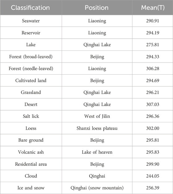
Table 1. Statistical analysis of temperature for typical normal-temperature objects on the surface with TIR data.
The SWIR temperature inversion method is based on physical models, whereas the TIR temperature inversion method employs the radiative transfer equation method in this article (Qin et al., 2001a; Qin et al., 2001b).
In practical applications, the DN value of the pixels in the SWIR remote sensing image, after radiation correction, represents the integrated electromagnetic radiation energy of the objects within the IFOV on the surface. For normal-temperature objects, the pixel DN value reflects reflected energy of the objects in the IFOV (in this condition, emission energy is neglected). For a mixed pixel composed of normal-temperature objects and high-temperature targets, the pixel DN value reflects the combined energy of the normal-temperature objects’ reflected energy and the high-temperature targets’ emitted energy. The equivalent reflectivity of the pixel caused by this integrated energy can be called visual reflectivity (Zhu et al., 2011).
The visual reflectivity of the mixed pixel represents the integrated electromagnetic radiation energy from the ground objects within the IFOV. According to the principle of energy conservation, it includes the reflected and emitted energy of the normal-temperature ground objects and the emitted and reflected energy of the high-temperature targets.
To simplify the model for practical application (Yu, 2017), the model assumes the following conditions:
All types of surface features are Lambertian. The normal-temperature ground features and high-temperature targets each have a uniform composition and temperature. The radiant energy from normal-temperature objects and high-temperature targets is linearly superimposed.
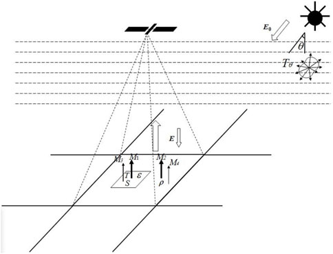
As a result, a physical model (Yu et al., 2016; Yu, 2017) for the SWIR temperature inversion of mixed pixels on the surface can be established (Figure 2).
Its mathematical expression is as follows (Equation 1):
In the formula, M is the radiation flux density of the mixed pixel, M1 is the emitted radiation flux density of the high-temperature target in the mixed pixel, M2 is the reflected radiation flux density of the normal-temperature objects in the mixed pixel, M3 is the reflected radiation flux density in the mixed pixel of the high-temperature target inside, M4 is the emitted radiation flux density of the normal-temperature ground object in the mixed pixel, and S is the area ratio of the high-temperature target in the mixed pixel.
In the SWIR spectrum, the radiation energy is primarily reflected by the sun, with a radiant brightness in the order of 10−1∼101 Wm−2 μm−1 ster−1. The background emission energy is very small, with a radiance in the order of 10−4∼10−3 Wm−2 μm−1 ster−1. The ratio of the reflected and emitted energy of the normal-temperature background in the SWIR is approximately 103:1. Therefore, the emitted energy of the normal-temperature background in the SWIR can be neglected (Pan et al., 2009; Zhu et al., 2011).
In summary, the SWIR radiation energy of mixed pixels consists of three components (Zhu et al., 2011): high-temperature target emission radiation, reflected radiation from the normal-temperature background, and reflected radiation from the high-temperature target. Thus, the mathematical expression of the physical model can be simplified (Equation 2).
For TIR temperature inversion of high-temperature targets, this paper adopts the radiation transfer equation method, also known as the atmospheric correction method (Qin et al., 2001a; Kafer et al., 2020). The basic idea is to use satellite-synchronized atmospheric data to estimate the degree of influence that surface thermal radiation has on the atmosphere. This influence is then subtracted from the total thermal radiation measured at the satellite’s entrance. Consequently, the thermal radiation intensity at the surface can be obtained. This intensity is then converted to the corresponding surface temperature.
The TIR radiance Lλ obtained by the satellite sensor consists of three parts. The first part is the upward atmospheric radiance L↑. The second part is the actual radiance of the Earth’s surface that reaches the satellite sensor after atmosphere’s effect. The third part is the downward atmospheric radiation L↓ whose reflected energy reaches the surface. The expression for the TIR radiance received by the satellite sensor is given by the following equation (Equation 3):
Among them, TS is the true temperature of the ground, B(TS) is the thermal radiance of a black body in TS derived from Planck’s law, and ε is the specific emissivity of the ground. The TIR radiance B(TS) of the black body at temperature T is as follows (Equation 4):
By entering the image acquisition time and positioning coordinates on the NASA website, the required parameters mentioned above can be obtained. These include the atmospheric transmittance Tθ, the upward atmospheric radiation L↑, and the downward atmospheric radiation L↓.
The energy of each component in the SWIR temperature inversion method is as follows:
1. The emitted radiation flux density M1 of the high-temperature target in the mixed pixel
According to the law of black-body radiation, the emission energy of the high-temperature target is the product of the emissivity ε of the high-temperature target and the Planck function B, that is (Equation 5),
In the formula, ε is the emissivity of the object; λ is the wavelength;
2. The reflected radiation flux density M2 of the ground objects at normal temperature in the mixed pixel
In the formula (Equation 6), ρ is the reflectivity of the ground objects at normal temperature, Tθ is the atmospheric transmittance, E is the solar irradiance at the surface, E0 is the upper boundary solar irradiance of the atmosphere, θ is the solar zenith angle, and ds is the solar-terrestrial astronomy unit distance.
3. The reflected radiation flux density of the high-temperature target in the mixed pixel M3 (Equation 7)
4. The total radiant flux density of mixed pixels M (Equation 8)
Combining these energy components into the formula yields the temperature inversion formula as follows (Equation 9):
Based on experience, remote sensing data are classified into three types of coverage. They are water, town, and natural surface. The following methods are used to obtain the surface specific emissivity of the study area. In these methods, the emissivity of water bodies is assigned a value of 0.995. The estimated emissivity values for natural surfaces and towns are calculated using Formulas 10, 11, respectively.
In the formula, εsurface and εbuilding represent the emissivity of natural surfaces and towns, respectively, and Fv is the vegetation coverage.
The vegetation coverage Fv is obtained using the mixed pixel decomposition method. The coverage types of the entire study area are roughly divided into water bodies, vegetation, and buildings. The specific calculation formula is as follows (Equation 12):
Among them, NDVI is the normalized difference vegetation index (Huete et al., 2002). NDVIv = 0.70; NDVIS = 0.00. When the NDVI of a pixel is greater than 0.70, the Fv value is 1. When the NDVI is lower than 0.00, Fv is 0.
After obtaining the radiance of the black body with a temperature of TS in the TIR band, using the inverse function of the Planck formula, the true ground temperature TS (Equation 13) is determined.
For the ETM + data TIR band, K1=666.09 W/(m2·sr·μm) and K2 = 1,282.71 K. For the Landsat 8 data TIR band, K1 = 774.89 W/(m2·sr·μm) and K2 = 1,321.08 K.
3 Study area and data
To make a strong statement in a comparative analysis study, two study areas are selected here. One is located at the junction of Baode County and Fugu County, and the other is in Xingcheng city.
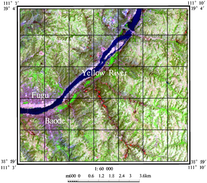
The first study area is located at the junction of Baode County in Shanxi Province and Fugu County in Shaanxi Province. They are on both sides of the Yellow River (Figure 3) (110°3′∼111°10′E, 38°59′∼39°4′N). The area contains coal seams in all layers, and it includes relatively abundant coal resources. Around 2002, the area was generally populated with various high-temperature targets, such as coke ovens and metal smelters (Yu et al., 2013). Most of the local coking plants were located at the bottom of loess gullies, while a few were situated on the loess beams, ridges, idle fields, and wastelands. In general, they are close to the coking coal-producing area and the water source. Therefore, the ETM + image (Goodwin and Collett, 2014) from Landsat 7 on 14 July 2002 was selected as the basic data for this research. The data were processed through radiometric calibration, atmospheric correction, projection transformation, and image cropping. The nominal wavelength λ of the ETM+7 band is 2.208 μm; the upper boundary solar irradiance of the E0 atmosphere is 82.1 Wm−2 μm−1 in the ETM + SWIR band; the sun zenith angle θ can be obtained from the image header file, and it is 27.24°. The temperature of the upper layer of the focal point can reach 500∼1,470 K. Moreover, during some special periods in the production process, the temperature exceeds 1,400 K.
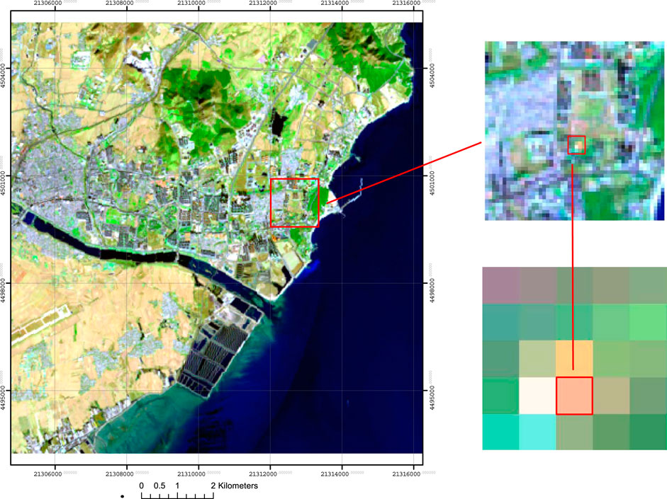
The second study area is located in the Xingcheng city of Liaoning Province (Figure 4) (120°06′∼120°50′E, 40°16′∼40°50′N). A synchronization satellite observation experiment was conducted there (Yu et al., 2016; Yu, 2017). The Landsat 8 OLI data from 9 November 2014 were selected as the basic data for this research. The nominal wavelength λ of the OLI seventh band is 2.201 μm. The area of high temperature is 4 m2. It consists of 20 stoves, each measuring 1 m × 0.2 m. The high-temperature stoves are placed in a large outdoor area (Figure 5), which is approximately 60 m × 90 m in size.
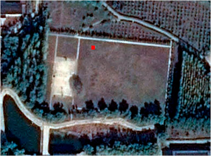
Figure 5. Remote sensing image of the experiment area from Google (the red rectangle on the image is the location of high-temperature targets).
In the physical model of the SWIR high-temperature mixed pixel, several parameters are considered, including atmospheric transmittance Tθ, normal-temperature ground object reflectivity ρ, and high-temperature target emissivity ε. The accuracy of these parameters is directly related to the accuracy of temperature inversion. The primary function of atmospheric transmittance Tθ is to calculate the total energy of the mixed pixels. The primary function of the reflectivity ρ of the normal-temperature object is to subtract the reflected energy from the total energy. High-temperature target emissivity ε is used to calculate the emitted energy. Inverting the performance temperature relies on the accurate determination of all parameters, which play a crucial role in SWIR temperature inversion. The parameters for TIR temperature inversion can be calculated using data from the NASA website and image pixel values.
3.1 Calculation of atmospheric transmittance
The atmospheric transmittance can be obtained through MODTRAN (Ni et al., 2022; Yang G. et al., 2023; Yang M. et al., 2023). MODTRAN is an atmospheric radiation transmission simulation model developed by the U.S. Air Force Geophysics Laboratory. It can be used to simulate radiance and atmospheric transmittance in the range of 50,000 cm−1 with a spectral resolution of 2 cm−1. By setting surface parameters, atmospheric parameters, sensor parameters, observation geometry parameters, control operating parameters, and output parameters, MODTRAN can accurately simulate the radiance at the top of the atmosphere.
The main parameter settings are as follows (Yu, 2014):
Based on the data, the mid-latitude summer atmospheric model is selected for the study area. The surface Kelvin temperature is 294.82 K. The ground object reflectivity at normal temperature is 0.45. The CO2 volume mixing ratio is 395.000. The rural aerosol mode is selected. The average ground elevation of the study area is 0.5 km. The height of the ETM + sensor is higher than 705 km. The altitude of the upper boundary of the MODTRAN atmosphere is 100 km. The average surface altitude is 0.5 km. ETM+ is a vertical observation with an observation angle of 180.000. The imaging time is July 14, and the calculated ‘day of the year’ is 195. The radiation source is the sun. The sub-satellite latitude is 38.91°. The longitude of the sub-satellite point is converted to a western longitude of 248.43°. Greenwich Mean Time for imaging is 3:00. The initial wavelength is 1,300 nm. The final wavelength is 2,500 nm. The wavelength increment is 10 nm. FWHM is 20. Radiance must be output. The output wavelength unit is nanometer (nm).
3.2 Background reflectivity estimation
Based on the principle of geographic correlation, we can calculate the reflectivity of the normal-temperature ground object within the high-temperature mixed pixel (Kitichotkul et al., 2024). The reflectance of normal-temperature objects within the mixed pixel should have the greatest possible spectral consistency and similarity with the nearest normal-temperature object pixel. This method is called the reflectivity estimation method of background pixels (Yu, 2017).
The reflectivity estimation method for background pixels employs two schemes for comparative analysis. One scheme involves remote-sensing image pixel sampling and statistical analysis. This method is based on the identification of high-temperature target (Fan et al., 2004) mixed pixels. The reflectivity of the surrounding neighboring pixels in the SWIR band needs to be measured and analyzed. The calculated value for the normal-temperature ground object is then used as the reflectivity. The other scheme is the object spectroscopy measurement method. In the satellite synchronous observation experiment, the normal-temperature background object’s spectrum is measured. Using the spectral response function of the satellite’s remote sensor, reflectance data are obtained, which serves as the calculated value for the normal-temperature ground object’s reflectivity (when there are more than two types of objects, a linear spectrum superposition model is applied). In this study, we use the former method to estimate the background reflectance.
3.3 Emissivity estimation of the high-temperature target
The emissivity of high-temperature targets is calculated by the measured spectral reflectance of the samples (Barducci and Pippi, 1996; Bastiaanssen et al., 1998; Aires et al., 2002; Atitar and Sobrino, 2009; Li et al., 2013; Zhang et al., 2023). The inverse of this is emissivity. Various high-temperature targets, such as coal, charcoal, coke, wood, vegetation leaves, grass, straw, steel, and volcanic rock, are used in field and laboratory experiments. The spectrum was measured, and the emissivity was determined (emissivity = 1-reflectivity). Various measured data serve as the empirical spectrum library for SWIR emissivity of high-temperature targets. The emissivity of non-metallic materials does not change with temperature under Earth’s environmental temperature conditions. A consensus has been reached. The emissivity spectrum data obtained under the normal-temperature conditions can be used as a reference for the emissivity of high-temperature ground objects. (Chen et al., 2000).
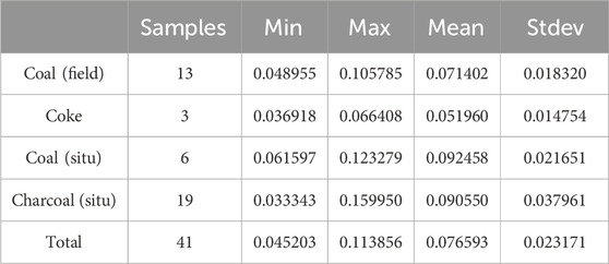
In this study, the emissivity of coal, char, and coke at normal temperatures is used in place of high-temperature emissivity. A near-infrared mineral analyzer is used to perform spectral testing on field-collected samples of coal, charcoal, and coke. The obtained spectral data are regarded as the reflectance of high-temperature targets. The spectrometer measures a spectral range of 1,300–2,500 nm, with a scanning interval of 2 nm. Forty-one field-collected samples were selected and converted into on-board data, according to the spectral response function (Table 2). The substitute value for emissivity was calculated using an inverse calculation method.
The imaging time of the Landsat 7 ETM + image in the study area was 3:00 on 14 July 2002. The latitude and longitude of the image center were 39.04°N and 111.11°E. For the atmospheric profile, we selected the mid-latitude summer model and Landsat 7 band 6 as the spectral response curve. On entering the data above into the NASA official website, the atmospheric transmittance Tθ of the TIR band is 0.83. The upward atmospheric radiance L↑ is 1.20 W/(m2·sr·μm), and the downward atmospheric radiance L↓ is 2.04 W/(m2·sr·μm).
According to the parameter above, the atmospheric transmittance Tθ, the normal-temperature ground object reflectivity ρ, and the high-temperature target emissivity ε are obtained. For the local coking method, the area of high-temperature targets is uncertain. For this reason, the proportion of the high-temperature target area is assumed to be 0.1, 0.5, and 1. These proportions are used as the critical area ratios for temperature inversion (Table 3). Using this parameter for temperature inversion of 200 high-temperature target pixels in the study area image, the temperature inversion statistics results in different areas can be found in Tables 4–6.
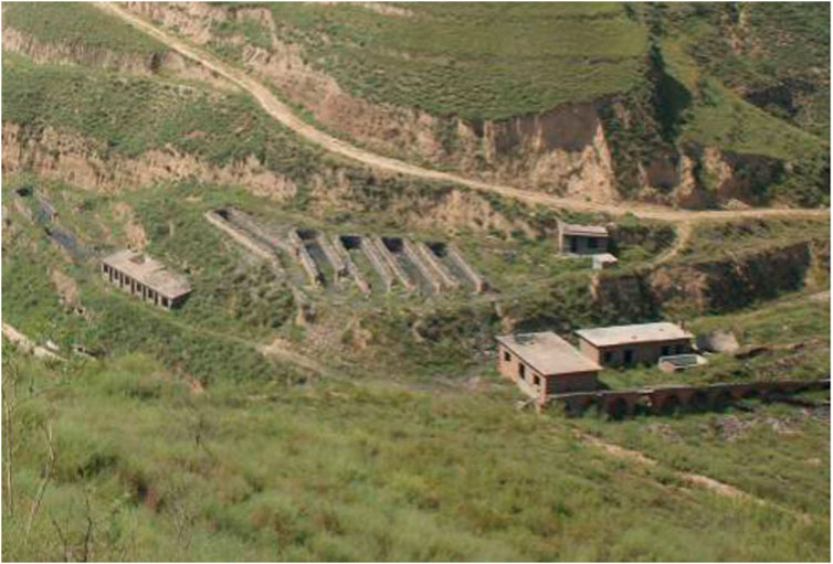
Field verification shows that the size of the indigenous coke oven is 10 m × 3 m, and most coking plants have approximately 5–7 coke ovens (Figure 6). The ratio of the high-temperature target area to the area of each pixel in the Landsat 7 image for the local coking method is approximately 0.1∼0.2. The SWIR temperature inversion result is closer to the actual value when the area ratio reaches a critical value of 0.1 (Table 4).
Parameters for the second study area are listed below. According to the satellite transit time of Landsat 8 at 10:41:07 Beijing time on 9 November 2014, the parameters for Xingcheng city, Liaoning Province, are shown below. The atmospheric transmittance, retrieved using the MODTRAN model, is 0.943. The reflectance of charcoal samples is measured using an ASD FieldSpec thermodetector. The average value is used to compute an integral on the basis of Landsat 8’s spectral response function and to convert the value to satellite reflectance of Landsat 8. After obtaining the emissivity of high-temperature targets (charcoal) in the SWIR band, ε is obtained as 0.9311 based on the formula ε = 1−ρ. The reflectance of grass and soil samples is measured using an ASD FieldSpec thermodetector. The fractional areas of grass and soil are computed based on outdoor photographs. According to the linear superposition model of spectra, spectral reflectance data for grassland are obtained. The integral is computed based on Landsat 8’s spectral response function, and the value is converted to Landsat 8 satellite reflectance. Finally, the reflectivity (ρ) is determined to be 0.0799.
4 Results and discussion
4.1 The first study area
The pixels that match the Landsat 7 TIR data for the aforementioned 200-pixel points are used to define the TIR temperature anomaly area. The other pixels serve as the normal-temperature background area for temperature inversion. The statistics for high-temperature targets and the background are as follows (Tables 7, 8).
Low-temperature distillation temperature for local coking is approximately 773.15 K (Yu et al., 2014c). In the local coking method, the TIR high-temperature target temperature inversion result ranges from 313 K to 334 K (mean value 319.00 K from Table 7). The relative error is 58.8%. The corresponding normal temperature background temperature inversion result ranges from 290 K to 331 K. The normal temperature background is relatively close to the temperature of the high-temperature target. These two results are easy to confuse. The SWIR temperature inversion result, ranging from 496 K to 651 K (mean value is 622.16 K from Table 4), is closer to the actual temperature of the high-temperature targets. The relative error is 19.5%. Furthermore, SWIR data can more accurately invert the temperature of high-temperature targets than TIR data. By examining the parameter settings of the two temperature inversion methods and the statistical data on the results, it is evident that the SWIR temperature inversion method inverts the temperature of high-temperature targets under various area ratios. In contrast, the TIR temperature inversion method directly calculates the overall high temperature. This represents the temperature inversion for mixed pixels. The emissivity used in temperature inversion has a specific range of applicability and is suitable only for normal-temperature ground objects. However, it introduces certain errors when used to invert the temperatures of high-temperature targets. Apparently, the TIR inversion method struggles to accurately reflect the temperature of high-temperature targets.
4.2 The second study area
We can see one high-temperature pixel in Figure 4, which is marked with a red square. It is the pixel where we have placed high-temperature stoves. Pixels adjacent to it are also affected, and these pixels display a different color compared to other normal-temperature pixels in the vicinity. The satellite Landsat 8 passed over the study area at 10:41:07 Beijing time on 9 November 2014. We found the transit time of Landsat 8 for the study area on the NASA website 2 days prior to the experiment. Twenty stoves were measured one by one using a portable thermodetector, and we measured the temperature many times. The two measurements (the last time before satellite transit and the first time after satellite transit, as shown in Table 9) are used as the actual temperatures for high-temperature targets. Finally, high-temperature targets and normal-temperature surface features are sampled, respectively. The spectral samples are measured indoor. High-temperature targets were the spare charcoal pieces that we selected randomly, and the normal-temperature surface features are grasslands. We sampled grass and soil, took photographs of them, and recorded descriptions. Temperature of the high-temperature target is calculated by Formula 9, and the value is 912 K. The relative error is 3.3% compared to the mean value 882 K (which is the mean of 860 K and 904 K, and these values were measured with a portable thermodetector). The TIR high-temperature target temperature inversion result is 320 K. The corresponding normal-temperature background temperature inversion result ranges from 290 K to 331 K. The normal-temperature background is relatively close to the temperature of the high-temperature target. These two results are easy to confuse. SWIR data can more accurately invert the temperature of high-temperature targets than TIR data.
5 Conclusion
There is no obvious temperature anomaly in the TIR remote sensing image for the high-temperature targets of the native coking method. The analysis from the perspective of spatial resolution shows that TIR remote sensing has a resolution of 60 m × 60 m, while the SWIR remote sensing image has a resolution of 30 m × 30 m. High-temperature targets with the same temperature and area are easily obscured by normal-temperature backgrounds in TIR remote sensing images. In particular, small-area high-temperature targets are more likely to be obscured by the background, making it difficult to distinguish them from the background. From the perspective of radiant energy and based on the black-body radiation law, the peak wavelength of normal-temperature objects is in the TIR range. Furthermore, the TIR band is more suitable for temperature inversion of normal-temperature objects. Additionally, TIR temperature inversion relies solely on the emitted energy of ground objects, while SWIR temperature inversion is based on the combined energy of emission and reflection of objects. Therefore, for the temperature inversion of high-temperature targets, the SWIR method is more advantageous. In particular, for small-area high-temperature targets, the SWIR method has more obvious advantages in temperature inversion.
TIR temperature inversion is the process of inverting the temperature of the entire pixel that contains the high-temperature target. However, it is inevitable that emissions from large areas of ambient-temperature background objects mix in, causing the energy of the high-temperature target to be evenly distributed across the mixed pixel, thereby reducing the temperature inversion value of the entire high-temperature pixel. On the other hand, SWIR temperature inversion is the process of inverting the temperature of the high-temperature target within the mixed pixels. The SWIR temperature inversion method is more conducive to high-temperature target analysis, such as resource investigation, environmental monitoring, and fire warning. At the same time, the study of SWIR temperature inversion methods also lays the foundation for further simultaneous inversion of temperature and area for high-temperature targets.
In the SWIR inversion of high-temperature targets, there is a certain error between the inversion result and the true temperature due to the approximate estimation of a key parameter: the area of the high-temperature target, as observed in the field. In future research, two shortwave infrared bands will be further utilized to simultaneously determine both the temperature and area. This approach aims to avoid the error caused by the key parameter, the area of the high-temperature target, in the inversion process and improve the accuracy of the inversion method.
Data availability statement
The raw data supporting the conclusions of this article will be made available by the authors, without undue reservation.
Author contributions
YY: data curation, formal analysis, investigation, resources, software, validation, visualization, writing–original draft, and writing–review and editing. JP: conceptualization, methodology, and writing–review and editing. HD: funding acquisition, project administration, supervision, and writing–review and editing.
Funding
The author(s) declare that financial support was received for the research, authorship, and/or publication of this article. This research was funded by the National Natural Science Foundation of China (No. 41871022), the Scientific Research Foundation for the doctor (No. 2018021), the young teachers’ scientific research ability cultivation promotion plan, and the Siping City Science and Technology Development Plan Project.
Conflict of interest
The authors declare that the research was conducted in the absence of any commercial or financial relationships that could be construed as a potential conflict of interest.
Publisher’s note
All claims expressed in this article are solely those of the authors and do not necessarily represent those of their affiliated organizations, or those of the publisher, the editors, and the reviewers. Any product that may be evaluated in this article, or claim that may be made by its manufacturer, is not guaranteed or endorsed by the publisher.
References
Adab, H., Kanniah, K. D., and Solaimani, K. (2013). Modeling forest fire risk in the northeast of Iran using remote sensing and GIS techniques. Nat. Hazards 65, 1723–1743. doi:10.1007/s11069-012-0450-8
Aires, F., Chédin, A., Scott, N. A., and Rossow, W. B. (2002). A regularized neural net approach for retrieval of atmospheric and surface temperatures with the IASI instrument. J. Appl. Phys. 41, 144–159. doi:10.1175/1520-0450(2002)041<0144:arnnaf>2.0.co;2
Atitar, M., and Sobrino, J. A. (2009). A split-window algorithm for estimating LST from meteosat 9 data: test and comparison with data and MODIS LSTs. IEEE Geosci. Remote S. 6, 122–126. doi:10.1109/LGRS.2008.2006410
Barducci, A., Guzzai, D., and Marcoionni, P. (2004). Comparison of fire temperature retrieved from SWIR and TIR hyperspectral data. Infrared Phys. Technol. 4 (1-2), 1–9. doi:10.1016/j.infrared.2004.03.001
Barducci, A., and Pippi, I. (1996). Temperature and emissivity retrieval from remotely sensed images using the “grey body emissivity” method. IEEE Geosci. Remote S. 34, 681–695. doi:10.1109/36.499748
Bastiaanssen, W. G. M., Menenti, M., Feddes, R. A., and Holtslag, A. A. M. (1998). A remote sensing surface energy balance algorithm for land (SEBAL). 1. Formulation. J. Hydrol. 212-213, 198–212. doi:10.1016/S0022-1694(98)00253-4
Biswal, S., and Gorai, A. K. (2020). Change detection analysis in coverage area of coal fire from 2009 to 2019 in Jharia Coalfield using remote sensing data. Int J Remote Sens 41 (24), 9545–9564. doi:10.1080/01431161.2020.1800128
Chen, F. L., Zhuang, J. L., Xu, X. R., Niu, Z., Zhang, R., and Xiang, Y. (2000). The concept of effective emissivity of nonisothermal mixed pixel and its test. Chin. Sci. Bull. 45 (9), 788–795. doi:10.1007/BF02887403
Dennison, P. E., and Matheson, D. S. (2011). Comparison of fire temperature and fractional area modeled from SWIR, MIR, and TIR multispectral and SWIR hyperspectral airborne data. Remote Sens Environ. 115 (3), 876–886. doi:10.1016/j.rse.2010.11.015
Di Biase, V., and Laneve, G. (2018). Geostationary sensor based forest fire detection and monitoring: an improved version of the SFIDE algorithm. Remote Sens. 10, 741. doi:10.3390/rs10050741
Ehsani, M. R., Arevalo, J., Risanto, C. B., Javadian, M., Devine, C. J., Arabzadeh, A., et al. (2020). 2019-2020 Australia fire and its relationship to hydroclimatological and vegetation variabilities. Water 12 (11), 3067–3118. doi:10.3390/w12113067
Ermida, S. L., Soares, P., Mantas, V., Göttsche, F. M., and Trigo, I. F. (2020). Google Earth engine open-source code for land surface temperature estimation from the Landsat series. Remote Sens. 12 (9), 1471–1526. doi:10.3390/rs12091471
Fan, X. L., Cheng, X. F., and Xu, J. (2004). High temperature target recognition based on spectral radiation information. Eng. Sci. 6 (6), 57–62. doi:10.3969/j.issn.1009-1742.2004.06.009
Giglio, L., Kendall, D., and Tucker, C. (2000). Remote sensing of fires with the TRMM VIRS. Int J Remote Sens 21 (1), 203–207. doi:10.1080/014311600211109
Goodwin, N. R., and Collett, L. J. (2014). Development of an automated method for mapping fire history captured in Landsat TM and ETM+ time series across Queensland, Australia. Remote Sens Environ 148, 206–221. doi:10.1016/j.rse.2014.03.021
Guo, J., Ren, H., Zheng, Y., Lu, S., and Dong, J. (2020). Evaluation of land surface temperature retrieval from Landsat 8/TIRS images before and after stray light correction using the SURFRAD dataset. Remote Sens. 12 (6), 1023. doi:10.3390/rs12061023
Hashimoto, A., Segah, H., Yulianti, N., Naruse, N., and Takahashi, Y. (2021). A new indicator of forest fire risk for Indonesia based on peat soil reflectance spectra measurements. Int J Remote Sens 42 (5), 1917–1927. doi:10.1080/01431161.2020.1846225
Huete, A., Didan, K., Miura, T., Rodriguez, E., Gao, X., and Ferreira, L. (2002). Overview of the radiometric and biophysical performance of the MODIS vegetation indices. Remote Sens Environ 3 (1-2), 195–213. doi:10.1016/S0034-4257(02)00096-2
Kafer, P. S., Rolim, S. B., Heinz, L. V. O., Iglesias, M. L., da Rocha, N. S., and Diaz, L. R. (2020). Assessment of single-channel algorithms for land surface temperature retrieval at two southern Brazil sites. J App Remote Sens 14 (1), 1–16. doi:10.1117/1.JRS.14.016507
Kitichotkul, R., Rapp, J., and Goyal, V. K. (2024). The role of detection times in reflectivity estimation with single-photon lidar. IEEE J.Sel.Topics Quantum Electron. 30 (1), 1–14. doi:10.1109/JSTQE.2023.3333834
Kong, X. S., Miao, F., and Liu, H. F. (2005). Dynamic monitor of indigenous coke-production using multitemporal Landsat remote sensing images: a case study in south-east, Shanxi province. Remote Sens Tech App 20 (5), 460–464. doi:10.396/j.issn.1004-0323.2005.05.001
Laneve, G., Pampanoni, V. S., and Riyaaz, U. (2020). The daily fire hazard index: a fire danger rating method for mediterranean areas. Remote Sens. 12 (15), 1–17. doi:10.3390/rs12152356
Laneve, G., Santilli, G., and Luciani, R. (2019). Improving SEVIRI-based hotspots detection by using multiple simultaneous observations. IEEE J-STARS 12 (7), 2349–2356. doi:10.1109/JSTARS.2019.2898126
Li, Z. L., Tang, B. H., Wu, H., Ren, H., Yan, G., Wan, Z., et al. (2013). Satellite-derived land surface temperature: current status and perspectives. Remote Sens. Environ. 131, 14–37. doi:10.1016/j.rse.2012.12.008
Lim, C. H., Kim, Y. S., Won, M., and Lee, W. K. (2019). Can satellite-based data substitute for surveyed data to predict the spatial probability of forest fire? A geostatistical approach to forest fire in the Republic of Korea. Geomat. Nat. Haz Risk 10 (1), 719–739. doi:10.1080/19475705.2018.1543210
Maithani, S., Nautiyal, G., Sharma, A., and Sharma, S. K. (2022). Simulation of land surface temperature patterns over future urban areas—a machine learning approach. J. Indian Soc. Remote Sens. 50, 2145–2162. doi:10.1007/s12524-022-01590-z
Ni, N., Zhang, K., Hu, J., Li, L., Mi, S., Zhang, Y., et al. (2022). Combined use of blackbody and infrared radiation for accurate measurement of temperature field of aluminum alloys. Optik 268, 169763. doi:10.1016/j.ijleo.2022.169763
Pan, J., Xing, L., X, , Wen, J. C., and Jiang, L. J. (2009). Inversion method study on short wave infrared remote sensing data high temperature surface feature temperature. 2nd CISP (6), 1–4. doi:10.1109/cisp.2009.5301511
Qin, Z. H., Karniel, A., and Berliner, P. (2001a). A mono-window algorithm for retrieving land surface temperature from Landsat TM data and its application to the Israel-Egypt border region. Int J Remote Sens 22 (18), 3739–3746. doi:10.1080/01431160010006971
Qin, Z. H., Zhang, M. H., and Arnon, K. (2001b). Mono-window algorithm for retrieving land surface temperature from Landsat TM 6 data. Acta Geogr. Sin. 56 (4), 456–466. doi:10.11821/xb200104009
Santana, N. C., Carvalhot Junior, O. A. D., Trancoso, G., and Renato, F. G. (2020). Comparison of post-fire patterns in brazilian savanna and tropical forest from remote sensing time series. Isprs Int. J. Geo-Inf 9 (11), 1–19. doi:10.3390/ijgi9110659
Schroeder, W., Ellicott, E., Ichoku, C., Ellison, L., Dickinson, M. B., Ottmar, R. D., et al. (2014a). Integrated active fire retrievals and biomass burning emissions using complementary near-coincident ground, airborne and spaceborne sensor data. Remote Sens Environ 140, 719–730. doi:10.1016/j.rse.2013.10.010
Schroeder, W., Oliva, P., Giglio, L., and Csiszar, I. A. (2014b). The New VIIRS 375 m active fire detection data product: algorithm description and initial assessment. Remote Sens. Environ. 143, 85–96. doi:10.1016/j.rse.2013.12.008
Sekertekin, A., and Bonafoni, S. (2020a). Land surface temperature retrieval from Landsat 5, 7, and 8 over rural areas: assessment of different retrieval algorithms and emissivity models and toolbox implementation. Remote Sens. 12 (2), 294–332. doi:10.3390/rs12020294
Sekertekin, A., and Bonafoni, S. (2020b). Sensitivity analysis and validation of daytime and nighttime land surface temperature retrievals from Landsat 8 using different algorithms and emissivity models. Remote Sens. 12 (17), 2776–2826. doi:10.3390/rs12172776
Shan, T. C., Zheng, W., Chen, J., and Tang, S. (2020). A burned area mapping method for the FY-3D MERSI based on the single-temporal L1 data and multi-temporal daily active fire products. Int J Remote Sens 42 (4), 1292–1310. doi:10.1080/01431161.2020.1826064
Stefanidou, A., Gitas, I. Z., Stavrakoudis, D., and Eftychidis, G. (2019). Midterm fire danger prediction using satellite imagery and auxiliary thematic layers. Remote Sens. 11 (23), 2786–2822. doi:10.3390/rs11232786
Szpakowski, D. M., and Jensen, J. L. R. (2019). A review of the applications of remote sensing in fire ecology. Remote Sens. 11 (22), 2638–2731. doi:10.3390/rs11222638
Veraverbeke, S., Stavros, E., and Natasha, H. S. J. (2014). Assessing fire severity using imaging spectroscopy data from the Airborne Visible/Infrared Imaging Spectrometer (AVIRIS) and comparison with multispectral capabilities. Remote Sens Environ 154, 153–163. doi:10.1016/j.rse.2014.08.019
Wright, R., Rothery, D. A., Blake, S., Harris, A. J. L., and Pieri, D. C. (1999). Simulating the response of the EOS Terra ASTER sensor to high-temperature volcanic targets. Geophys Res. Lett. 26 (12), 1773–1776. doi:10.1029/1999GL900360
Xu, G., and Zhong, X. (2017). Real-time wildfire detection and tracking in Australia using geostationary satellite: himawari-8. Remote Sens. Lett. 8 (11), 1052–1061. doi:10.1080/2150704X.2017.1350303
Xu, Y., Fan, H. D., and Dang, L. B. (2021). Monitoring coal seam fires in Xinjiang using comprehensive thermal infrared and time series InSAR detection. Int J Remote Sens 42 (6), 2220–2245. doi:10.1080/01431161.2020.1823045
Yang, G., Yu, Y., Sun, Z., Li, Z., Pang, X., and Zhang, T. (2023). Radiometric calibration algorithm for high dynamic range infrared imaging system. Infrared Phys. Technol. 130, 104607. doi:10.1016/j.infrared.2023.104607
Yang, M., Xu, L., Tan, X., and Shen, H. (2023). A method based on blackbody to estimate actual radiation of measured cooperative target using an infrared thermal imager. Appl. Sci. 13, 4832. doi:10.3390/app13084832
Yin, S., Wang, X. F., Guo, M., Santoso, H., and Guan, H. (2020). The abnormal change of air quality and air pollutants induced by the forest fire in Sumatra and Borneo in 2015. Atmos. Res. 243 (1), 105027–105113. doi:10.1016/j.atmosres.2020.105027
Yu, X., Guo, X., and Wu, Z. (2014c). Land surface temperature retrieval from Landsat 8 TIRS—comparison between radiative transfer equation-based method, split window algorithm and single channel method. Remote Sens. 6 (10), 9829–9852. doi:10.3390/rs6109829
Yu, Y. F. (2014). The study of high-temperature targets temperature retrieval model in shortwave infrared remote sensing. Changchun: Jilin University.
Yu, Y. F. (2017). The SWIR remote sensing retrieval of high-temperature targets about physics parameter. Changchun: Jilin University.
Yu, Y. F., Pan, J., and Xing, L. X. (2013). Identification of high temperature targets in remote sensing imagery based on mahalanobis distance. Remote Sens. Info 26 (5), 90–94. doi:10.3969/j.issn.1000-3177.2013.05.017
Yu, Y. F., Pan, J., and Xing, L. X. (2014a). Feasibility analysis of shortwave infrared band for recognition of high temperature target. Remote Sens Land Resour. 26 (1), 25–30. doi:10.6046/gtzyyg.2014.01.05
Yu, Y. F., Pan, J., Xing, L. X., Jiang, L., and Yu, H. (2016). Study of high temperature targets identification and temperature retrieval experimental model in SWIR remote sensing based Landsat8. Int. J. Appl. Earth Obs. 46, 56–62. doi:10.1016/j.jag.2015.11.011
Yu, Y. F., Pan, J., and Xing, L. X. I. (2014b). Dentification of high temperature targets in remote sensing imagery based on factor analysis. J. Appl. Remote Sens. 8, 1–8. doi:10.1117/1.JRS.8.083622
Zhang, Z., Chen, M., Zhang, L., Li, H., Huang, H., et al. (2023). A straightforward spectral emissivity estimating method based on constructing random rough surfaces. Light Sci. Appl. 12, 266. doi:10.1038/s41377-023-01312-1
Keywords: thermal anomalies, multispectral data, remote sensing, small areas, temperature inversion
Citation: Yu Y, Pan J and Du H (2024) Comparative analysis of high-temperature targets retrieved from SWIR and TIR data. Front. Environ. Sci. 12:1446007. doi: 10.3389/fenvs.2024.1446007
Received: 08 June 2024; Accepted: 30 October 2024;
Published: 19 November 2024.
Edited by:
Venkata Ravibabu Mandla, National Institute of Rural Development and Panchayati Raj, IndiaReviewed by:
Shaohua Zhao, Ministry of Ecology and Environment Center for Satellite Application on Ecology and Environment, ChinaSurendra Sharma, Indian Institute of Remote Sensing, India
Copyright © 2024 Yu, Pan and Du. This is an open-access article distributed under the terms of the Creative Commons Attribution License (CC BY). The use, distribution or reproduction in other forums is permitted, provided the original author(s) and the copyright owner(s) are credited and that the original publication in this journal is cited, in accordance with accepted academic practice. No use, distribution or reproduction is permitted which does not comply with these terms.
*Correspondence: Huishi Du, ZHVoc0BqbG51LmVkdS5jbg==
 Yifan Yu1
 Huishi Du