- 1Institute for Infrastructure and Environment, School of Engineering, The University of Edinburgh, Edinburgh, United Kingdom
- 2Centre for Environment, Fisheries and Aquaculture Science (CEFAS), Lowestoft, United Kingdom
- 3National Oceanography Centre, Liverpool, United Kingdom
- 4Department of Biological and Environmental Sciences, University of Stirling, Stirling, United Kingdom
- 5National Oceanography Centre, Southampton, United Kingdom
- 6NOVELTIS, Labège, France
Understanding and monitoring sea surface salinity (SSS) and temperature (SST) is vital for assessing ocean health. Interconnections among the ocean, atmosphere, seabed, and land create a complex environment with diverse spatial and temporal scales. Climate change exacerbates marine heatwaves, eutrophication, and acidification, impacting biodiversity and coastal communities. Satellite-derived ocean colour data provides enhanced spatial coverage and resolution compared to traditional methods, enabling the estimation of SST and SSS. This study presents a methodology for extracting SST and SSS using machine learning algorithms trained with in-situ and multispectral satellite data. A global neural network model was developed, leveraging spectral bands and metadata to predict these parameters. The model incorporated Shapley values to evaluate feature importance, offering insight into the contributions of specific bands and environmental factors. The global model achieved an R2 of 0.83 for temperature and 0.65 for salinity. In the Gulf of Mexico case study, the model demonstrated a root mean square error (RMSE) of 0.83°C for test cases and 1.69°C for validation cases for SST, outperforming traditional methods in dynamic coastal environments. Feature importance analysis identified the critical roles of infrared bands in SST prediction and blue/green colour bands in SSS estimation. This approach addresses the “black box” nature of machine learning models by providing insights into the relative importance of spectral bands and metadata. Key factors such as solar azimuth angle and specific spectral bands were highlighted, demonstrating the potential of machine learning to enhance ocean property estimation, particularly in complex coastal regions.
1 Introduction
Sea surface salinity (SSS) and sea surface temperature (SST) are both essential climate variables for monitoring ocean health Reul et al. (2020). This is particularly important for the global coastal ocean, which impact coastal communities through provisioning, regulating, supporting, and cultural ecosystem services. Ocean, atmosphere, seabed and land (also ice in high latitudes) are all interconnected in the coastal ocean. This creates a complex and highly variable environment, the dynamics of which operate over a wide range of spatial (mms to 100 km) and temporal (seconds to centuries) scales, Malik and Harmel (2016), Melet et al. (2020). Global warming is leading to an increase in intensity and frequency of marine heat waves, eutrophication and acidification events which not only affect biodiversity but also impact coastal communities through food, human health and economic activities, Oliver et al. (2018), Paul et al. (2012), Minnett et al. (2019), Breitburg et al. (2018). These can result in: disruption to marine ecosystems including, fish migration, coral bleaching and habitat loss; algal blooms, followed by oxygen depletion zones; and decarbonisation of foundational mollusc species. All of which have knock on effects on those communities which rely through food or economy on these ecosystems.
Existing monitoring strategies, primarily reliant on in situ observations from buoys and depth profiles, have limitations in capturing the full spatial and temporal variability of SSS and SST, especially in coastal areas, Jin Woo and Park (2020), Mann et al. (2017). While these methods provide accurate results for mean conditions and diurnal variability, they struggle to depict sub-mesoscale processes like river plumes, coastal eddies, and algal blooms, Dickey and Bidigare (2005), Muller-Karger et al. (2018). Moreover, remote sensing techniques, such as microwave and infrared satellite observations from platforms like Soil Moisture Ocean Salinity (SMOS) and Soil Moisture Active Passive (SMAP), offer broader spatial coverage but lack sufficient resolution for coastal monitoring, particularly in regions with salinity variations, Font et al. (2010), Babin et al. (2004), Dickey (2008). Satellite-derived ocean colour provides the opportunity to estimate sea surface properties with significantly improved spatial coverage compared with in-situ monitoring, and with pixel resolution on the ten to hundred metre scale compared to traditional microwave remote sensing kilometric to decakilometric scale, Hadjal et al. (2022).
Ocean colour estimation of temperature, salinity and other sea surface properties involves inferring the water properties from the spectral signature emitted by the water leaving radiance
Accurate retrieval of water-leaving reflectance from satellite imagery requires robust atmospheric correction techniques. These techniques, including scene-based measurements, empirical line approaches, and radiative transfer models, are essential for extracting accurate water-leaving reflectance values from satellite data, Gao et al. (2014). However, performing atmospheric correction in coastal zones presents unique challenges due to non-Lambertian surfaces and complex atmospheric effects such as cloud masking, sun glint, and aerosol variability, He and Pan (2003), or from radiance outside the field of view of the pixel (adjacency effects). Moreover, accurate atmospheric correction often necessitates information on in-situ aerosol size and particle behavior, which can be challenging to obtain, particularly in inaccessible regions, Frouin et al. (2019). Six publicly available ATM correction algorithms Acolite, C2RCC, iCOR, l2gen, Polymer and Sen2Cor, were tested in coastal and inland waters, Warren et al. (2019). All were found to have high uncertainties particularly in the red and near-infrared bands.
Work has been done on estimating SST and SSS from ocean colour satellite images with no atmospheric corrections Medina-Lopez (2020). Using Sentinel 2 Level 1-C TOA (Top of Atmosphere) data as the input to a Neural network, 2.4 showed an improvement over the Bottom of Atmosphere (BOA) 2-A data product which was corrected by the Sen2Cor processor. The BOA data was shown to be only accurate in open waters, possibly due to the poor coastal applicability of the ocean atmospheric correction models. This improved accuracy of TOA products could be due to the information content lost when applying typical atmospheric correction models to satellite data. A machine learning algorithm with increased training and test data is generally more accurate, with the caveat of training data quality. This poses an interesting question as to the necessity of atmospheric corrections for SST or SSS ocean colour inference, the increased information content of TOA and lack of poor atmospheric corrections in coastal waters, sun glint and whitecaps versus the selection of water leaving radiance from the overall irradiance at the satellite sensor.
Therefore this paper introduces a methodology to extract SST and SSS from multispectral ocean imagery, linking top-of-atmosphere radiance to these variables. Global in situ data records of SST and SSS from the Copernicus marine in situ database as well as the Gulf of Mexico and UK are matched with Sentinel-2 satellite information. Several machine learning algorithms, including gradient boosting, decision tree regressors and neural networks, are used to estimate the sea surface parameters with Sentinel-2 spectral bands and metadata properties as input to the models. The machine learning algorithms were tested regionally and globally to predict SST and SSS from the spectra independently. Finally, feature weighting methods are used to understand the importance of various inputs in the models predictions.
2 Materials and methods
2.1 In-situ sea surface temperature and salinity data
This section introduces dataset statistics for two independent datasets from the UK and the Gulf of Mexico, as well as global SST and SSS from the Copernicus in-situ monitoring system, CMEMS TAC Data Team (2021). These datasets are used as the training data for the final machine learning algorithms. The globally sourced data encompasses a wide range of coastal environments, including nearshore regions, estuaries, and coastal shelf seas. These provide insights into the variability of SST and SSS across different latitudes. This enables the regional-dependent variations in these parameters, such as the influence of ocean currents, atmospheric circulation, and coastal geography, to be examined. Moreover, this work provides coverage at a higher spatial resolution, providing benefits for coastal regions or regions with high spatio-temporal variability not captured by current remote sensing technologies. Although the global data is useful to provide increased match-ups and data, the UK and Gulf of Mexico were chosen due to their proximity to shore and estuarine conditions, as well as the variable temperature and salinity distributions that they provide.
2.1.1 UK smart buoy data
The UK estuary data provides a temperate water study region, made up from buoys in Liverpool Bay, Dowsing, West Gabbard and the mouth of the Thames (Southend-Sheerness) (Figure 1). The rivers in these locations have less freshwater input compared to major European rivers (like the Rhine or the Danube) and Amazonian rivers, Blöschl et al. (2019). However, Liverpool Bay, in particular, exhibits clear freshwater influence, Howarth et al. (2005), making it an ideal location to study small-scale ocean dynamics and their implications for coastal ecosystems. UK smart buoy data is obtained from the Centre for Environment, Fisheries and Aquaculture Science of the UK (Cefas),Cefas (2024). As there is no overlap between the global data and the UK data, this works well as a test case. It also provides a good juxtaposition with the study in the Gulf of Mexico, which experiences 15–20° warmer temperatures on average and has very different tidal dynamics (averaging 0.3–0.6m tidal range), impacting the magnitude of saltwater intrusions, Mejia-Olivares et al. (2020), Robins et al. (2016).
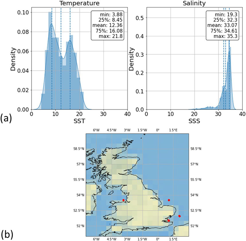
Figure 1. (A) Distribution of temperature and salinity parameters for the UK smart buoy dataset: 800 and 400 data points for the SST and SSS distributions, respectively. (B) Locations of UK Smart Buoys, Cefas (2024).
2.1.2 Gulf of Mexico coastal observing system
The Gulf of Mexico, particularly the Florida Keys region, is an important environmental ecosystem with unique and diverse marine life. However, it is vulnerable to problems ranging from eutrophication, overfishing and loss of habitat, Guiry et al. (2021), Paerl and Otten (2013), Halpern et al. (2008). This has further impacts on coastal erosion and increased vulnerability to extreme weather events, Pennings et al. (2021), such as tropical cyclones, without the protection from mangroves or other natural barriers, Alongi (2008). The Gulf of Mexico was chosen as a study for its varied waters, including shallow coastal bays and deeper offshore regions, which provide an excellent opportunity to study the dynamics of coastal ecosystems. These areas are characterized by their proximity to land, complex bathymetry, and diverse marine habitats. The Gulf of Mexico Coastal Observing System (GCOOS) uses NOAA cruises and stations to monitor estuaries in the Gulf of Mexico Coastal Ocean Observing System (2024). The large number of estuaries and tributaries from the Mississippi affect the Gulf, making it useful training data for temperature and salinity ranging from 0 to 35° and freshwater to fully saline at 35.5 PSU. The model data produced will enable assessments of SST and SSS temporal variability, which has impacts on the health of coral reefs, mangroves, and other sensitive habitats, as well as aiding monitoring complex ecosystems in the region that will be affected by large changes in temperature and salinity.
Figure 2 shows the range of temperature and salinity values for the Gulf of Mexico. This presents large variations, showing the average value for each buoy reading, from the cooler fresh water near the coast to the warmer saline ocean water. This is an interesting case study because it seems to show that temperature and salinity are inversely linked. However, it is important to note that this relationship is just based on the average reading for the Gulf, this relationship will change seasonally and is dependent on other conditions. To avoid seasonal imbalances the number of match-ups was checked to ensure it was consistent throughout the year. Furthermore, as the model inputs included the Reflectance Correlation Coefficient (RCC) metadata, this can be used as a proxy for seasonality and the model could learn patterns due to seasonal shifts. This approach enhances the model’s ability to generalize across diverse seasonal and regional conditions, mitigating the effects of data imbalance. Temperature and salinity are measured separately, which is why there are different number of data points and distributions for each of the variables.
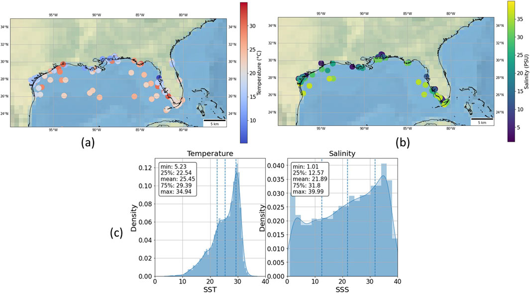
Figure 2. (A) Range of temperature values for Gulf of Mexico. (B) Range of salinity values for Gulf of Mexico. (C) Distribution of temperature and salinity parameters for the Mexico datasets (8,000 and 5,000 points, respectively, for SST and SSS).
2.1.3 Global Copernicus marine environment monitoring service (CMEMS)
The global dataset comes from the Copernicus in situ Marine Environmental Monitoring Service (CMEMS) (with datasets coming from over 100 countries,. CMEMS provides datasets from various observing systems, including Argo float profiles, and observations from ships, moored buoys, drifting buoys, fixed platforms, gliders, ferry-boxes, and coastal observations. These datasets encompass a variety of oceanographic parameters such as temperature and salinity, SeaDataNet. All in-situ data was selected from the Copernicus marine database within the criteria of being less than 1m depth and having both SST and SSS continuous measurements. Figure 3 also shows the global spatial distribution of the Argo floats that were matched with a satellite image. There is higher frequency of observations in the nearshore regions with fewer open ocean buoys. This corresponds to the tasking path of the Sentinel-2 satellite discussed in Section 2.2. Sentinel-2 is primarily a land monitoring satellite European Space Agency (2019) which also captures the coastal zone with some values recorded over open ocean. This will skew our training data, however open ocean is a lot more homogeneous than coastal shelf seas. This also poses the question about the training data fed to the model: how valid is the feeding of open ocean data to the model? Is this altering the training distribution of SSS and SST values and making the model tend to predict “better fitting” points which match this open ocean but not the coastal waters? Furthermore the algorithms in this paper will only be applied in these coastal regions as in open ocean there is no need for higher spatial resolution than already available products, Chassignet and Xu (2021).
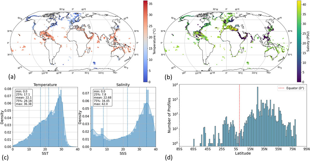
Figure 3. Map of matched Argo data points. (A) Temperature. (B) Salinity. (C) Distribution of temperature and salinity parameters for the global dataset (12,000 points). (D) Distribution of the buoys with respect to latitude.
Figure 3C shows temperature and salinity value distributions. The SST distribution is skewed with a mean temperature above 22°C, and salinity showing twin peaks of 35 PSU in open ocean and 0 PSU corresponding to freshwater readings. A significant percentage of these buoys are located in the global north and particularly on the coast of North America and around Europe (the North Atlantic and Mediterranean), see Figure 3D.
2.1.4 Data processing and quality inspection
All of the in-situ data were pre-processed using their respective quality flags and testing procedures. For the Copernicus data, only points with the quality QC1 flag were used relating to “good quality” data, CMEMS TAC Data Team [2021]. There is also extensive testing for each GCOOS data point, Gulf of Mexico Coastal Ocean Observing System (2024). UK smart buoy data are maintained by Cefas and regularly checked for bio-fouling. Data are subject to a full quality assurance procedure which assigns flags to poor quality data (e.g., for sensor malfunction, drift) Sivyer (2016).
Furthermore, statistical and environmental measures were employed for data cleaning purposes. As the distributions were non-normal, Median Absolute Deviation (MAD) was used to reject outliers which had a deviation from the median over 4 times the median of the all median deviations. Outliers beyond acceptable ranges were identified and rejected by defining boundaries based on historical data or climatological norms for each region. This involved analysing past observations to establish typical ranges of values for the variables of interest. Time-based anomaly detection was also used to identify anomalies or sudden spikes that may not be captured by traditional outlier detecting methods. Seasonal decomposition of the data into trend, seasonal and residual components allowed visualisation and analysis of the residuals with removal of fluctuations relating to anomalies.
2.2 Satellite imagery
The satellite utilized in this study is the European Space Agency (ESA) Sentinel-2 multispectral satellite system. Consisting of two satellites, Sentinel-2A and Sentinel-2B, it offers a revisit time of approximately 5 days at the equator, enabling frequent monitoring of Earth’s surface. Operating in a polar orbit, these satellites cover the entire globe, capturing high-resolution imagery for various applications. The Sentinel-2 data comprise 13 spectral bands, each represented as 16-bit unsigned integers (UINT16) and scaled by a factor of 10,000 to obtain top-of-atmosphere (TOA) reflectance values. The spectral bands include: coastal aerosol (443 nm), red edge detection (705 nm) and near infrared band (842 nm), and a full list is available here: European Space Agency (2023).
Sentinel-2 was selected due to its high spatial resolution of 10–60m, which enables high quality monitoring of the highly spatial variations seen in coastal regions. Sentinel-2 is part of the Copernicus monitoring programme, which is specifically looking at land monitoring. However, its high resolution, wide swath and spectral range enables monitoring of vegetation and water cover as well as coastal observations, European Space Agency (2019).
2.2.1 Satellite metadata
Sentinel-2 also provides metadata taken from the image collection. Including metadata such as reflectance conversion correction, incidence zenith angle, incidence azimuth angle, mean solar azimuth angle, and solar irradiance into the model inputs offers several advantages. Firstly, the reflectance conversion correction factor accounts for variations in Earth-Sun distance, ensuring that the reflectance measurements are consistent across different solar angles. This correction enhances the accuracy of the spectral data by allowing it to be normalised across standard condition, mitigating the effects of varying solar illumination angles. Secondly, the inclusion of incidence zenith and azimuth angles provides valuable information about the angle and direction of sunlight relative to the observed area. Moreover, the mean solar azimuth angle and solar irradiance offer insights into the intensity and direction of sunlight incident on the Earth’s surface during satellite observations. These parameters all influence the spectral response of surface features. Integrating metadata into the model inputs allows us to leverage additional information about environmental conditions and solar geometry, enhancing the interpretability and predictive performance of the machine learning algorithms. Since top-of-atmosphere spectral data is used, focusing on these metadata parameters aids in decoding the relationships between solar irradiance, atmospheric conditions, and observed reflectance values from the water column without explicitly modeling radiative transfer processes.
To streamline the input features and avoid redundancy, the band-specific metadata values were averaged into a single value. Giving a total of 18 inputs to the model, 13 spectral bands and five metadata features (mean solar azimuth angle, reflectance conversion correction, mean incidence zenith angle, mean incidence azimuth angle, solar irradiance). This process, known as feature aggregation, offers several benefits. First, it reduces the dimensionality of the input space, improving computational efficiency and mitigating the curse of dimensionality. Second, it helps smooth out noise or variability in the data, leading to more robust model predictions. Third, by capturing collective behavior or trends in the data, feature aggregation enhances the model’s generalization to new instances and unseen scenarios. Additionally, the aggregated features promote model interpretability by focusing on essential patterns and characteristics in the data. All the models included this metadata as well as the pixel spectral data.
2.3 Matching process
All of the in situ datasets underwent the same matching process with the multispectral satellite images. The Sentinel-2 data was processed on the Google Earth Engine Python API platform. This allows geospatial analysis and processing of satellite images on Google Cloud computers, using scalable, high performance computing resources. However, there is additional data transfer costs and the inherent risks from depending on a third party provider, Google Earth Engine (2023). Latitude, longitude and time of measurement are taken for each in-situ data point. The Sentinel-2 image collection is filtered to the tiles that contain the point on the day and time when the measurement was taken, within 1 hour of Sentinel-2 overpass. One hour was chosen to improve accuracy, especially in the coastal zones where tidal effects and river flows can vary significantly over the course of hours.
The matched images for those points are clipped in 3 × 3 pixel windows about the in-situ data point, to retain the high resolution benefits from the Sentinel-2 satellite. The whole 3 × 3 pixel window is taken to avoid any random noise reflectance, wave effects or sun-glint errors occurring at the pixel level. The median value of the window for the spectral bands and metadata is then selected for the matched point. Time difference is also recorded between the in-situ measurement and satellite image, if there are multiple images within 1 h of the in-situ point the smallest time difference is selected. The output is a table containing all satellite data (spectral bands and metadata properties) with the corresponding salinity and temperature data. As mentioned in previous sections, for the Gulf of Mexico and UK data, SSS and SST were recorded separately and therefore the satellite match ups for each parameter are different.
2.3.1 Satellite data cleaning
The matched satellite image data was also subject to data cleaning and quality checks. Firstly, any satellite image with metadata ‘CLOUDYPIXELPERCENTAGE’ (percentage of the overall satellite image covered in cloud) above 60
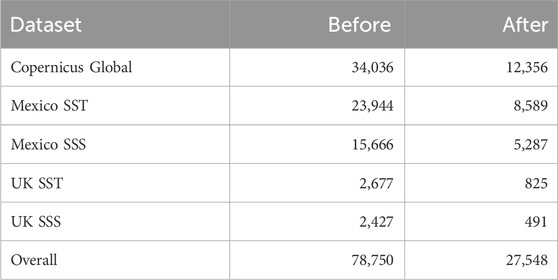
Table 1. Number of satellite match ups before and after cloud and statistical in-situ data cleaning.
2.4 Machine learning techniques
Machine learning (ML) is the ability of an algorithm to learn and find out information and relationships in data, Pedro Domingos (2012). Machine learning offers significant potential in various aspects of remote sensing and specifically the field of oceanography. One key advantage lies in its ability to handle large and complex datasets, extracting valuable insights from vast amounts of Earth observation data collected by satellites like Sentinel-2. The more input and training data an algorithm has access to, the more it can learn about the properties of that data, Sonnewald et al. (2021), Ali et al. (2020). Satellite data, with its constant monitoring, provides a large temporally varying dataset, with large spatial and data variability, highly suitable for machine learning purposes, Belgiu and Drăguţ (2016).
2.4.1 Gradient boosting models
Gradient Boosting models offer a powerful tool for analysing complex datasets. Gradient Boosting models operate by iteratively combining weak learners, such as decision trees, to improve predictive accuracy. These models focus on minimizing errors by sequentially adding trees, each addressing the residual errors of the previous ones, Friedman (2001). XGBoost (eXtreme Gradient Boosting), is an example of a specific scalable distributed gradient-boosted decision tree (GBDT) structure. It can further enhance model performance through regularization techniques, handling missing data, and parallel computation, Chen and Guestrin (2016). By aggregating the strengths of individual trees, each leaf improving the residual errors, XGBoost is able to capture intricate patterns and non-linear relationships within the data. Its popularity arises from its scalability, speed, and robustness, hence its attraction in applications including remote sensing and environmental modeling, Hosseiny et al. (2022).
2.4.2 Neural networks
Neural networks are layered structures linking the input variables via interconnected neurons to an output estimate or class, through a number of hidden layers, as shown in Figure 4. At each layer of the network, neurons learn the weights from the outputs of a logistic regression. The advantage of such a structure is that by a combination of these interconnected layers, the network can find non-linear relationships between variables to a high order. Neural networks are excellent for the environmental challenges with large amounts of data and to uncover complex relationships, Hsieh (2009).
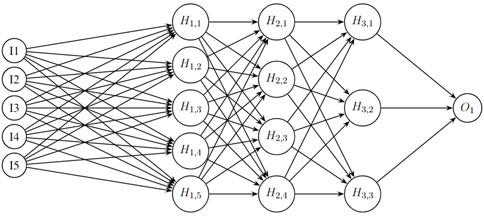
Figure 4. Neural Network architecture - with three hidden layers, five inputs and one output node. Each individual neuron in each layer is formed by the sum of all the neurons in the previous layer (with separate weights) convolved with some non-linear activation functions.
Neural networks have been used to estimate SST and SSS in coastal waters. Using neural networks removes the need to find or define specific inherent optical properties, andf therefore SSS and SST can be directly estimated from apparent optical properties, removing the need for specialised radiative transfer models. The factors in the accuracy and successful test validation are the quantity and quality of training data, and the tuning of the networks hyperparameters such as hidden layer number, loss functions and inputs selected. A grid search method was employed to determine optimal hyperparameters such as learning rate, batch size, and number of hidden layers. Learning rates were tested in the range of 0.001–0.01, and batch sizes of 32, 64, and 128 were experimented with. The final chosen hyperparameters of 0.1 learning rate and batch size 128 were based on minimizing validation loss while avoiding overfitting. Three such neural networks for the estimation of SSS are discussed here and details compared in Table 2. All of these except Medina-Lopez and Ureña-Fuentes (2019) require SST as an input to the model to predict SSS.
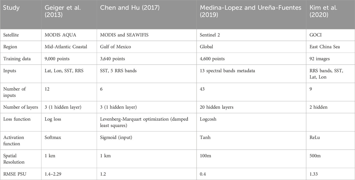
Table 2. Comparison of Neural Network structures for predicting SSS. Based on satellites: MODIS AQUA (Parkinson (2003)), SEAWIFS (Gregg et al. (1997)), Sentinel-2 (European Space Agency (2019)) and Geostationary Ocean Colour image (GOCI) (Ryu et al. (2012)).
Neural networks can learn complicated relationships, producing SSS and SST purely from satellite and location information, however, care must be taken when selecting inputs and training data to capture the full variance of values. Furthermore, including location to inputs can limit generalisation of model to new regions, as well as the model learning the “wrong” relationships. Therefore, in this instance, latitude and longitude are not taken as inputs to the model, certain locations are excluded from the training set to validate true generalisation, and, in the k-fold validation care was taken to ensure the samples were geographically stratified. Overly complex architectures may exacerbate overfitting. Additionally, adjustments to parameters like learning rate and batch size can impact training convergence and efficiency. Therefore, careful tuning and validation are essential to strike the right balance between model complexity and generalization performance.
2.4.3 Algorithm comparison
The algorithm development methodology was the same for all the datasets. First, simpler regression algorithms were applied to see if there was any correlation between spectra and ocean properties, then decision tree, gradient boosting and XGBoost models were tested for each dataset. Hyperparameterisation was explored to maximise models performance and behaviour, such as increased “max depth” in decision trees, which controls the complexity of the decision tree. This can help capture more intricate patterns in the data, potentially leading to better performance. However, this can lead to overfitting on training data if “max depth” is too large, causing the model to capture noise or outliers. Training time and computational resources also increase with a higher number of estimators, making the model slower to train and predict. Learning rate was also adjusted, with smaller rates facilitating smoother convergence by controlling step size, effectively acting as a regularisation, with usual caveats for computation cost and slower convergence and training time.
The DecisionTreeRegressor (DTR) performed better than simpler regression models due to its ability to capture non-linear relationships. By increasing the max depth parameter, the model could capture more intricate patterns. However, a larger max depth risks overfitting, as the model may start to fit noise or outliers. Best performance was achieved with max depth = None, allowing the tree to grow fully and improve fit, while avoiding significant overfitting due to the nature of the dataset.
The Gradient Boosting Regressor, (GBR) consistently outperformed the DTR due to its ensemble learning approach, which combines weak learners to produce a stronger model. With max depth = 10 and n estimators = 50, the model captured complex patterns in the data without significant overfitting. The learning rate = 0.1 ensured smooth convergence, acting as a regularization mechanism to prevent the model from making overly aggressive updates. The combination of weak learners allowed the GBR to generalize well, balancing model complexity and performance. The AdaBoost Regressor (ABR), performed well with n estimators = 300, allowing it to combine a high number of weak learners. However, like the DTR, this approach risks overfitting when weak learners try to fit noise in the data. Despite this risk, the ABR showed good performance by improving its predictive power through ensemble learning, though it required more regularization than GBR to prevent overfitting. The XGBoost model (XGB), with max depth = 6 and n estimators = 100, struck a balance between complexity and generalisation. Its ability to handle missing values, optimize gradient boosting algorithms, and regularize during training made it particularly well-suited for this dataset. The relatively smaller max depth (compared to GBR) and more controlled number of estimators helped prevent overfitting while maintaining strong predictive capabilities. XGBoost’s advanced optimization techniques and flexibility allowed it to deliver competitive results with relatively efficient training times.
Finally, neural networks were employed to use the non-linearity behaviour to capture the complex second order relationships, as well as methods to understand uncertainty in the predictions. In this study, a feed-forward neural network architecture with multiple hidden layers (10) was designed, with a Tanh activation function to for propagating non-linearities. As before, 18 nodes were used for the neural network initial layer to match the input data of bands and metadata. Dropout regularisation helped prevent overfitting, while early stopping, based on validation set performance, further ensured that the model did not overtrain on the noise in the data. Additionally, the max-pooling layers, improved model ability to extract relevant information and improve generalisation performance. Training the network with stochastic gradient descent (SGD) and optimizing with mean squared error (MSE) allowed for more efficient convergence over the course of 1,000 epochs, resulting in a model that outperformed traditional methods like gradient boosting and XGBoost. The neural network’s ability to capture complex, non-linear dependencies between features made it the most effective approach for this study.
All the models were trained with a 70% training 30% test data split, then subject to k-fold cross validation where k = 5, where the model was trained on four folds and validated on the remaining fold, rotating through all folds. The models were all trained using RMSE as the error metric and were validated on RMSE as well as RME, MAE and MPSE. Finally for each regional model as well as the global model certain buoy locations were withheld from the model allowing it to perform validation on unseen locations.
3 Results and discussion
The structure of this section will consider each of the dataset studies individually with a comparison and discussion on general applicability at the end. Table 3 shows the Root-Mean-Square Error (RMSE) and other metrics for each of these algorithms developed for SST. Every algorithm used 18 inputs as previously described, the 13 spectral bands and five averaged metadata values. The XGBoost model was also tested on purely spectral bands to better visualise how important metadata inclusion is to model performance and to increase understanding of the band and surface properties relationships.
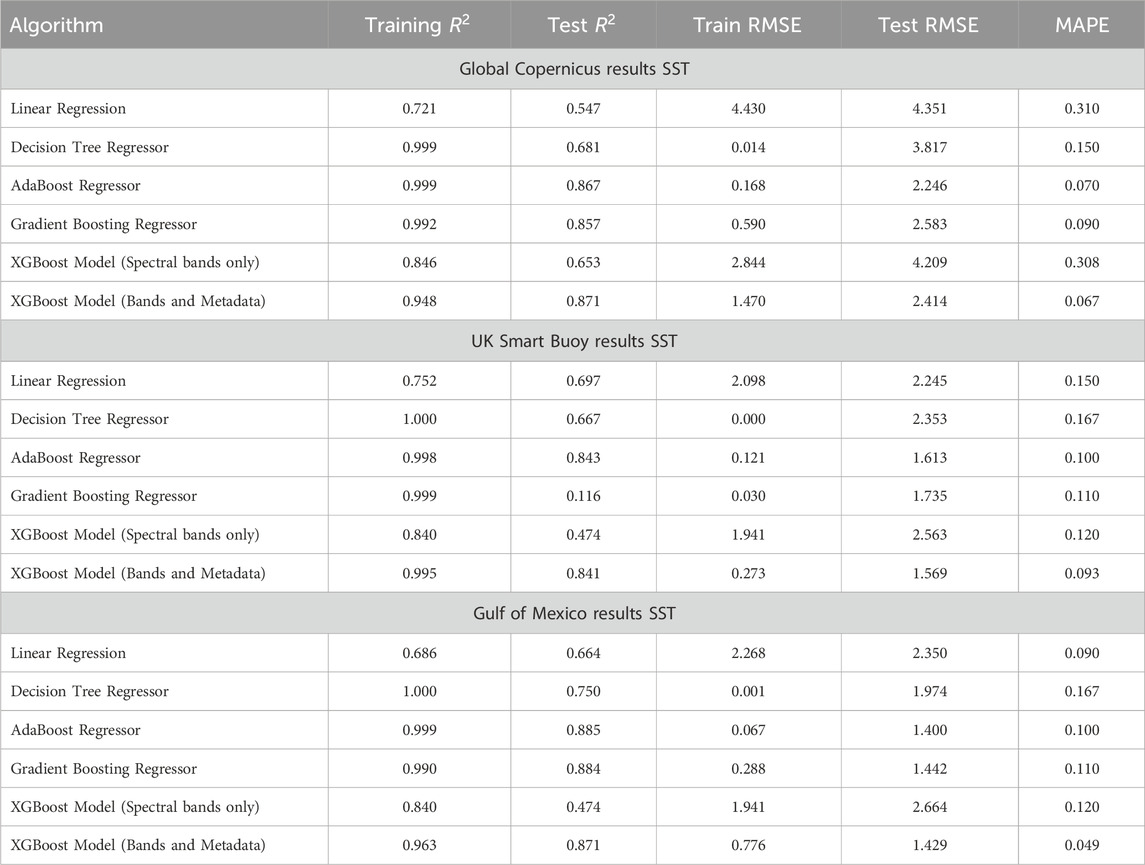
Table 3. Sea surface temperature prediction Errors for Different Machine Learning Algorithms. Model results for linear regression, decision tree and gradient boosting regressors. Results for the Global Copernicus, the UK Smart buoy and Gulf of Mexico datasets. Coefficient of determination
In the UK, where training data is relatively limited compared to other regions, the models exhibit varying levels of performance. The Linear Regression model shows moderate accuracy with a Test RMSE of 2.786, suggesting reasonable predictive capability despite the simplicity of the model. Conversely, more complex models like Decision Tree Regressor and Gradient Boosting Regressor, while achieving lower Test RMSE values (3.251 and 2.323 respectively), also demonstrate potential overfitting due to the small dataset size. This indicates a need for caution in interpreting their results, as they may not generalize well to unseen data.
In contrast, linear regression failed to capture even true training data information and could not predict test datasets for the other cases. Particularly in the global dataset with such varied input ranges. The predictive models for Mexico and the global dataset show more consistent performance, with Test RMSE values ranging from 1.593 to 3.5638. The higher Test RMSE values in global data compared to the Gulf of Mexico, contrasting with their similar SST distributions show the impact on the model on such diverse oceanic conditions and environmental factors in global data. Despite the AdaBoostRegressor had the best test RMSE of all the algorithms with 1.59 in Mexico. This was discarded in favour of the XGB model (test RMSE 1.70) due to the computational training and running times the XGB having over a 20 time faster runtime.
Figure 5 shows scatter plots of actual vs the XGB model predicted SST (from Tables above) for the test datasets (data not seen by the model during training) for the UK, Mexico and global. Most of the predictions show generally good correlation with certain outliers for each case. There is obvious sparsity and smaller range in the UK data, corresponding to less buoy match ups and cooler waters.
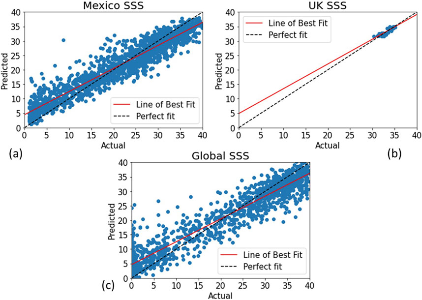
Figure 5. XGBoost model scatter plots of predicted vs actual temperature values for unseen validation data. (A) Gulf of Mexico (B) UK Smart buoy and (C) Global Copernicus data.
Across the three scenarios, the prediction of SSS presents unique challenges compared to SST (Figure 6). In the global dataset, which encompasses diverse oceanic conditions, the machine learning models exhibits poor performance in predicting SSS. The UK Smart Buoy dataset stands out with very high accuracy in RMSE errors for all algorithms including linear regression due to its relatively small range of SSS values. However, while these results are promising for the UK Smart Buoys, it is essential to recognize that the model’s performance may not generalize well to datasets with broader ranges of salinity values. This discrepancy between SST and SSS prediciton capabilities may be attributed to the availability of suitable spectral bands for each parameter. Temperature estimation can leverage shortwave infrared (SWIR) and infrared bands.
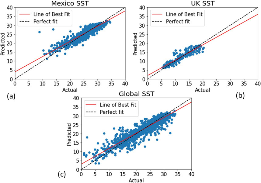
Figure 6. XGBoost model scatter plots of predicted vs actual salinity values for unseen validation data. (A) Gulf of Mexico, (B) UK Smart buoy and (C) global data.
3.1 Testing algorithm in specific platforms
In this section, we focus on analyzing the seasonal cycles evident in the temperature data collected from various locations. By testing the XGBoost (XGB) model on these sites, we aim to understand how well it captures the seasonal variations in temperature. Exploring the temporal patterns and seasonal variations in the residuals between actual and predicted SST values could provide valuable insights into the model’s ability to capture underlying trends and improve its predictive accuracy over time.
Figure 7A Shows the results of an XGB model tested on the Liverpool buoy location, (data not used for training). There is good coherence between predicted (blue) and real (orange) data points, and seasonal cycles are captured (RMSE 0.421). Figure 7B shows the buoy location with the most datapoints for Mexico, NOAA.NDBC:GBIF1 and predicted SST results for the platform. Figure 7C shows the XGB global model performing on platform Wee1 at (latitude 25.23, longitude −80.99, off the coast of North America).
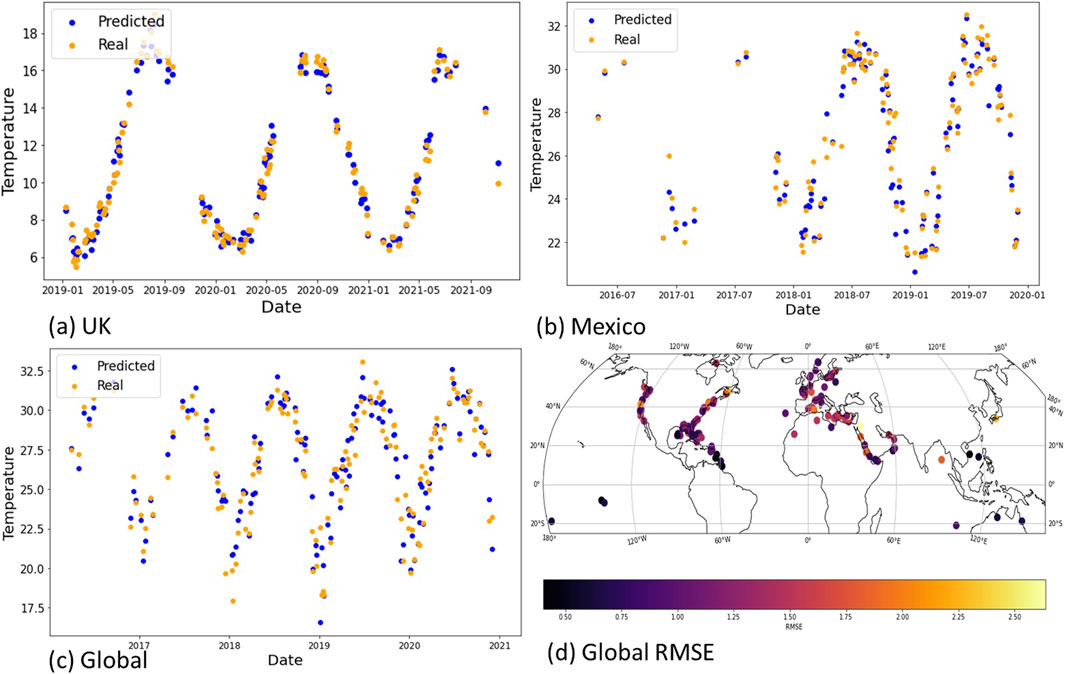
Figure 7. Temperature platform plots for unseen locations. (A) UK model tested on Liverpool buoy data (trained on the other three locations). (B) Mexico model Platform NOAA.NDBC:GBIF1. (C) Global platform WWEF1 at (latitude 25.23, longitude −80.99). (D) Mean RMSE for the global platforms for temperature.
Figure 8 shows the predicted vs real estimates for SSS in the same unseen buoy locations as tested for SST before. Interestingly, the platform in Mexico and the buoy in the global data pick up their representative underlying seasonal signals (fresh water influence in winter), despite the high RMSE shown in Table 4. Figure 8D shows the RMSE for locations for the global dataset, showing strong model performance in North America and Europe (location with more data points) and weaker in areas with lower data availability, such as the Arabian Gulf.
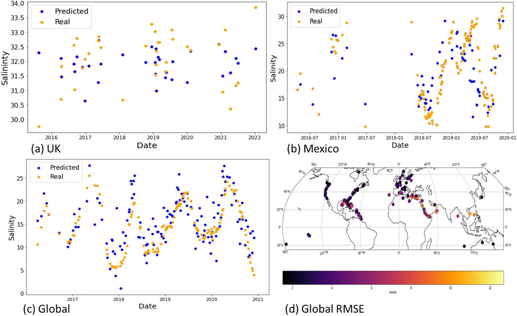
Figure 8. Salinity platform plots for unseen locations. (A) UK Liverpool bay buoy. (B) Gulf of Mexico platform NOAA.NDBC:GBIF1. (C) Global WWEF1 buoy, as in previous figures. (D) Mean RMSE platform errors for the global dataset.
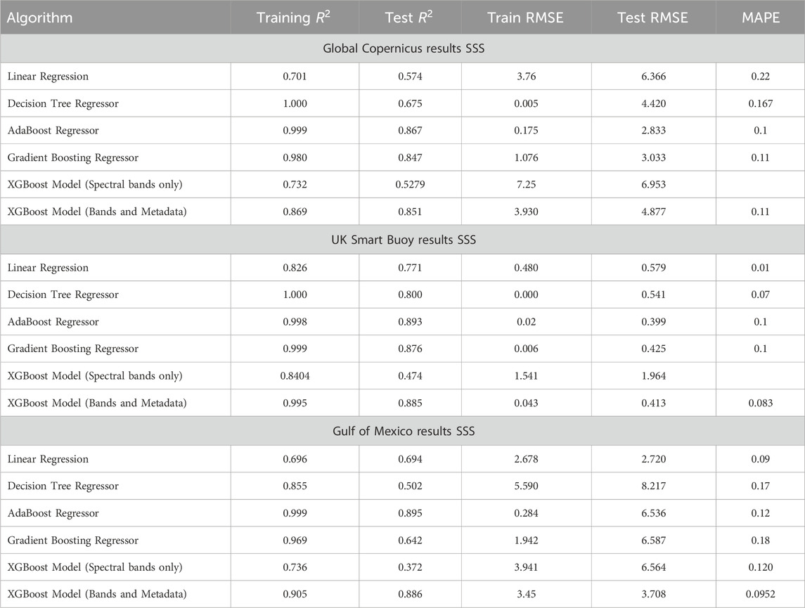
Table 4. Sea surface salinity prediction Errors for Different Machine Learning Algorithms. Model results for linear regression, decision tree and gradient boosting regressors. Results for the Global Copernicus, the UK Smart buoy and Gulf of Mexico datasets. Coefficient of determination
3.2 Neural network application
For the global neural network algorithm, temperature was predicted with a coefficient of determination
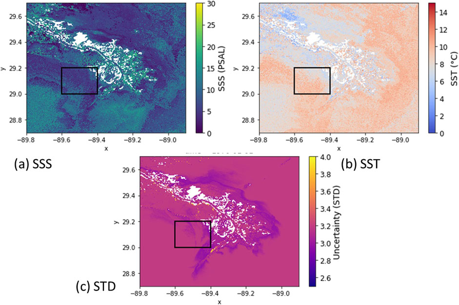
Figure 9. Neural Network image results from the Mississippi river in the Gulf of Mexico, land is masked out as white. (A) SSS (B) SST and (C) Uncertainty given by the standard deviation. The outlined bounding box is the subregion explored in Figure 10.
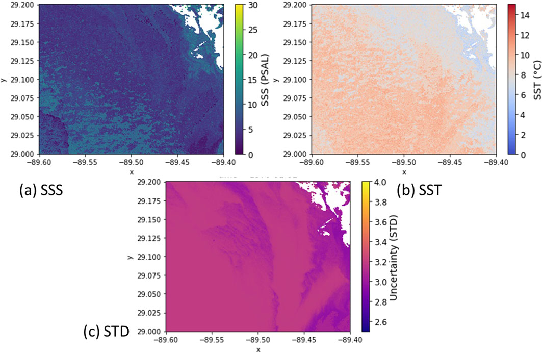
Figure 10. Subregion of the Missippi delta river. (A) SSS plot (B) SST, showing a front boundary (C) Uncertainty, spatial variation.
Figure10 shows the bounded region in Figure 9. 10 (a) shows the SSS plot, with the resolution of the product this now allows front and eddy features on the 100m scale to be identified, and the saline water feature close to land in the top right. 10 (b) shows the temperature gradient and front location that could not be seen at the coarser resolution.
Thermal and passive microwave sensors achieve higher accuracy when estimating temperature- the NASA Moderate Resolution Imaging Spectroradiometer MODIS and Advanced very-high-resolution radiometer (AVHRR) (RMSE of 0.43°C and 0.68°C, respectively, when validated against ferry observations on open ocean waters). However, neither of these sensors can observe coastal sites sampled by the coastal in-situ buoys used in this study due to land adjacency and resolution, and their resolutions at 4 km are very different to the decametric resolution of the model presented in this paper, making them unsuitable for a direct comparison with the methodology developed in this study. This highlights the need for future datasets designed specifically for coastal and near-shore environments to enable better validation of machine learning models in these areas. SSS was predicted in the global case study with a 15% uncertainty, at 10 m resolution. In highly variable coastal waters (0-36PSU range) this is sufficient to show seasonal or annual warming trends and detect key salinity fronts (such as river plume boundaries). The validation data was also split temporally by month without losing accuracy, implying the model learning seasonal variations well from the RCC metadata. As a comparison metric, the satellites Soil Moisture Ocean Salinity (SMOS) and Soil Moisture Active Passive (SMAP) perform well with open ocean data (0.25PSU uncertainty), but this is only tested in open ocean waters with salinity values ranging from 34 to 36PSU, and coastal regions are excluded due to insufficient resolution (40 km).
Accuracy could be improved by implementing model selection based on water type classification, more varied observations of different global regions, and closer matched satellite and in-situ data points. The algorithm is not trained on historical data to inform the present or future SST or SSS variables to save computational time. To therefore ensure that the model is learning from long term trends particularly with regards to ocean warming care must be taken to continually update the training data.
3.3 Algorithm explainability
The use of machine learning algorithms, such as XGBoost and neural networks used in this paper, has become increasingly popular in various fields, including oceanography, to predict oceanic parameters. However, one of the drawbacks of these models is the lack of transparency, often referred to as the “black box” problem, where it is difficult to understand how the model arrived at its predictions. This can pose significant problems in model’s acceptance and uptake by the ocean science community who distrust the opaqueness of purely data based models without a strong physical parameterisation basis. Feature selection offers a solution to this problem by identifying the most important features used to predict the target variable. Typically used in reducing the dimensionality of the data, feature selection not only improves the model’s performance and mitigates the risk of overfitting, but can also provides crucial insights into the underlying relationships within the data. This has an advantage over common feature reduction methods such as Principal Component Analysis (PCA) by retaining the original features not producing new orthogonal dimensions. An example is the XGBoost feature importance. This measures the relative importance of each feature in the XGBoost model by calculating the average gain of each feature across all decision trees in the ensemble. The gain of a feature is the improvement in the objective function (e.g., reduction in loss function error) attributed to that feature when a split is made on that feature. The higher the gain, the more important the feature is viewed. While this approach is useful to determine influential features by ranking on feature importance scores, which can be used as a pre-processing step to select the
3.3.1 SHAP values
SHapley Additive exPlanations (SHAP values) Lundberg and Lee (2017) offer a solution to these problems by providing a better understanding of how different features contribute to the final prediction. We will explore the use of SHAP values for feature extraction in model creation and how they can provide a better understanding of the underlying physics involved in predicting SST and SSS from multispectral satellite images. SHAP values offer both global and local interpretability. Not only do they indicate the importance of each feature in making predictions, but they also reveal whether a feature has a positive or negative impact on those predictions. Unlike other techniques that provide only aggregated results over the entire dataset, SHAP values enable us to calculate feature contributions for individual predictions.
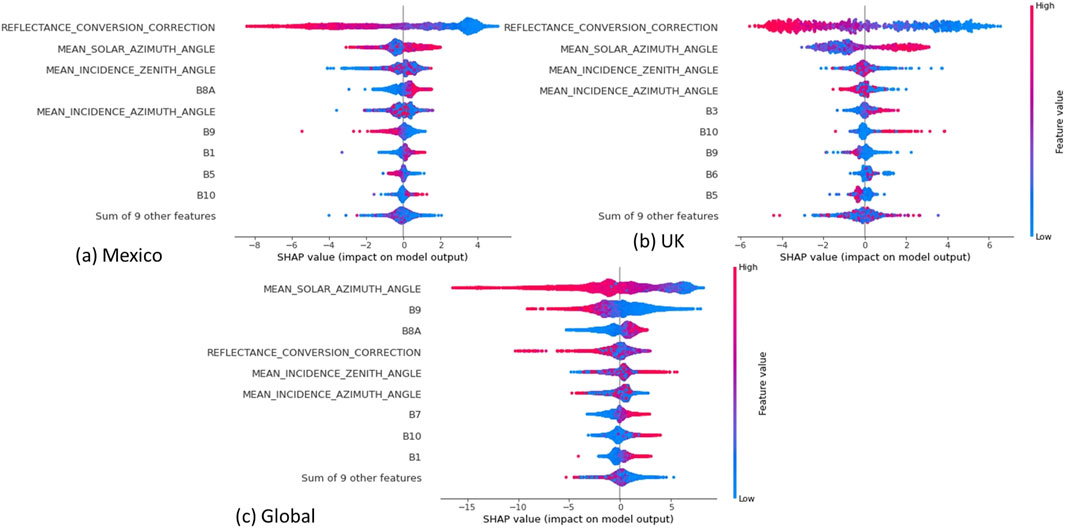
Beeswarm plots offer a unique visualization technique that provides insights into explaining the directional nature of the features. Figure 11 shows the beeswarm results for the inputs to the SST models, e.g., high reflectance correction coefficient (RCC) signifies winter (in northern latitudes) which gives a negative impact on the model output as seen before in Mexico and the UK. This directional insight aids understanding the underlying model computations, enhancing interpretability. Although RCC was the dominating input for both the UK and Mexico data, the Beeswarm plot distributions shows more UK values in the tails. The absolute SHAP values are different for each location due to the differences in temperature range: the UK with a range of around 15° shows accordingly less SHAP impact.
In Mexico, specifically, the plots indicated a cooling effect associated with high values of B9 and a warming effect linked to positive values of B8A on SST estimation. These findings suggest that variations in these specific bands have a discernible impact on SST dynamics in the region. An explanation for this could be as B9 is sensitive to water vapor absorption in the atmosphere. High values of B9 may indicate increased water vapor content in the atmosphere, leading to cooling effects on the sea surface temperature. Conversely, B8A, being in the near-infrared range (0.85–0.87 microns), is sensitive to reflectance properties of surface features, including vegetation. Positive values of B8A may indicate higher reflectance from surfaces or vegetation, resulting in increased heating of the sea surface due to greater solar radiation absorption.
These relationships are different dependent on location: in the UK, B10 (SWIR) has positive relationship with temperature, tracking the link between thermal radiation and warmer surface temperatures. While it is also positive in Mexico, it has a far less importance ranking, possibly due to higher prevalence of cloud in the warmer regions. They can also be opposing one another: B3 (the green part of the spectrum) in the UK has a positive correlation with SST. In the UK regions with abundant phytoplankton or suspended sediments, higher values of B3 may indicate increased absorption of solar radiation, leading to warmer surface temperatures. However, in Mexico, where the negative correlation occurs, divergence from the UK data could be due to differences in coastal ecosystems, water clarity, or phytoplankton abundance. Factors such as higher turbidity or phytoplankton blooms might lead to increased scattering and reduced absorption of solar radiation.
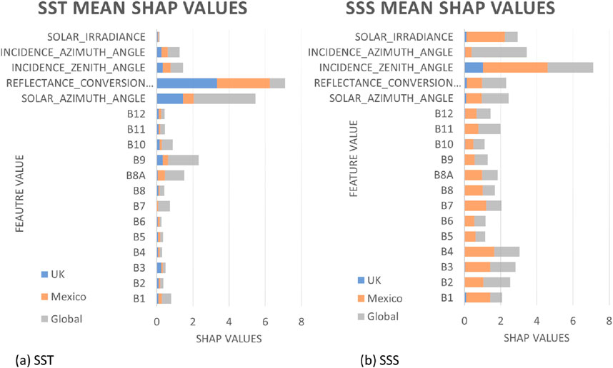
The mean SHAP values were calculated to determine the average absolute impact of selected features on the model’s predictions across all observations in the validation set (Figure 12). This metric provides insight into the overall contribution of each feature to the model’s predictions, irrespective of the direction of the effect. In analysing the Mean SHAP values, it was observed that different spectral bands exhibited varying degrees of importance in estimating SST and SSS across different water temperatures. In SST, specifically, in warmer waters, bands B9 and B11 demonstrated the most significant contribution to SST estimation, while in cooler waters, bands B11, B8A, and B6 emerged as crucial factors. The identification of these key bands underscores the importance of considering the spectral characteristics in enhancing the model’s accuracy, particularly under varying water temperature conditions. For the global SST estimation, the mean solar azimuth angle emerged as the most influential feature, as evidenced by its substantial mean SHAP value of 3.42. This was followed by bands B9 and B8A, which exhibited mean SHAP values of 1.7 and 1.06, respectively. For the Gulf of Mexico and the UK, RCC (representing the Earth-Sun distance metric) was the dominate input, linking to the strong seasonality in these regions opposed to the global data which is training on northern and southern hemispheres simultaneously.
For the SSS models, the mean incidence zenith angle (indicative of the time of day), and mean incidence azimuth angle were the most important features. The salinity SHAP values were also evenly spread over most inputs. Comparatively, the infrared bands (B7-B10) were less important than in the SST models, however, RGB bands were the most important spectra underlying the strong relationship between SSS and organic matter, e.g., chlorophyll. Mean B4 for global SSS was 1.5 compared to 0.14 for SST.
Conducting SHAP analysis on multiple regions can unveil patterns and trends in the importance of spectral bands and metadata features for SST and SSS estimation. When employing clustering techniques on the regional model, SHAP values could then identify similarities among water types, facilitating the development of more generalized models suitable for global applications. Additionally, investigating temporal changes in SHAP values, especially in regions exhibiting seasonality, can offer insights into the dynamic nature of predictions. Analysing how the importance of spectral bands and metadata features fluctuates overtime can enhance the understanding of seasonal variations in SST and SSS. Comparing SHAP values between temperature and salinity predictions can provide insights into the common and unique drivers influencing these variables. This understanding can be used to enhance the predictive capability of the models and shed light on the underlying physical processes governing ocean properties.
4 Conclusion
This paper has demonstrated the feasibility of estimating sea surface temperature and salinity from ocean colour satellite imagery. With SST predicted with a coefficient of determination
The use of SHAP values in this study provided valuable insights into the significance of spectral bands and metadata features for predicting both SST and SSS. The exploration revealed spatial variations in feature importance, shedding light on the underlying dynamics of oceanic properties across different locations. Leveraging this information holds promise for enhancing model accuracy by identifying key drivers for SST and SSS and allowing for a better understanding of the relationship between the two. For instance, identifying seasonal trends and variations in metadata values and subsequent feature importance, such as solar irradiance and zenith angles, could inform predictive models of temperature fluctuations. There is also the potential for calculating the SHAP values of additional environmental variables beyond ocean colour images in more complex climate models, e.g., including wind direction, speed and cloud cover as inputs in the predictive model and improving our understanding of the interaction between these physical parameters, the spectral signature and SST and SSS.
The methodology shown here can be used as a foundation to scaling to global model. However, the size of training data and selection of local vs global models play an essential role in the accuracy of models used for these efforts. Data availability remains a challenge, especially in remote regions, including polar regions, which have different distributions of SST and SSS due to the freshwater influence from the cryosphere, high latitude rainfall and climate. All of which can affect model performance due to variation from training data distributions. This would also require significant computational resources for processing and model training, particularly in the case of cloud-based platforms. Ocean colour also struggles in regions with high cloud coverage due to scarcity of observations compounded with the lack of training data, decreasing accuracy in these regions, such as the tropics with high cloud, large rainfall and the subsequent flooding or other land impacts on the coast. Machine learning through interpolation is helping to improve these points, but there is still a limiting degree of certainty. Future developments in sensing technology, such as hyperspectral satellites and geostationary satellites, hold promise for better temporal monitoring and improved coverage of different zones and the model accuracy improvements that increased data availability can bring.
4.1 Future steps
The methodology developed here can be applied to other multispectral or hyperspectral satellites as well as Sentinel-2 to further increase temporal and spatial coverage and better improve the accuracy of the SST and SSS products. Offering potential fusions with Sentinel-3 (with 300m resolution but daily revisit times) and NASA’s Landsat series. The development of NASA’s Plankton, Aerosol, Cloud, ocean Ecosystem mission (PACE), NASA, is an exciting stage in the global ocean colour coverage, Groom et al. (2019). This methodology could be further tested and refined using the upcoming PACE data, which is expected to provide enhanced spectral resolution and improved observations of global ocean colour. By leveraging the data from PACE, this approach has the potential to significantly improve the accuracy and spatial-temporal resolution of sea surface temperature (SST) and salinity (SSS) estimates. Additionally, future missions that build on the real-time processing and machine learning capabilities demonstrated here may focus on integrating advanced models for faster and more reliable monitoring of global ocean properties. Other work of interest is the combination of historical and present satellites across hyper and multispectral bands, (Barnes et al. (2015); Burggraaff (2020)), to produce long-term time series at high resolution to monitor the changing ocean and impact of anthropogenic activity. Furthermore, improving uncertainty quantification in model predictions can be achieved through Bayesian neural networks, offering probabilistic outputs that provide valuable insights into prediction reliability. This uncertainty quantification offers valuable insights into the model’s confidence in its predictions, particularly in regions where the data are sparse or noisy.
Data availability statement
The original contributions presented in the study are included in the article/supplementary material, further inquiries can be directed to the corresponding author.
Author contributions
SW: Conceptualization, Data curation, Formal Analysis, Investigation, Methodology, Software, Validation, Visualization, Writing–original draft, Writing–review and editing. TS: Supervision, Writing–review and editing. LA: Supervision, Writing–review and editing. ES: Supervision, Writing–review and editing. AM: Supervision, Writing–review and editing. EM-L: Supervision, Writing–review and editing.
Funding
The author(s) declare that financial support was received for the research, authorship, and/or publication of this article.
Acknowledgments
SW acknowledges Cefas as the PhD CASE partner for his PhD project. The PhD project was funded through the Centre for Satellite Data in Environmental Science (SENSE CDT) – funded by NERC and UK Space Agency.
Conflict of interest
Author AM was employed by the company NOVELTIS.
The remaining authors declare that the research was conducted in the absence of any commercial or financial relationships that could be construed as a potential conflict of interest.
Publisher’s note
All claims expressed in this article are solely those of the authors and do not necessarily represent those of their affiliated organizations, or those of the publisher, the editors and the reviewers. Any product that may be evaluated in this article, or claim that may be made by its manufacturer, is not guaranteed or endorsed by the publisher.
Supplementary material
The Supplementary Material for this article can be found online at: https://www.frontiersin.org/articles/10.3389/fenvs.2024.1426547/full#supplementary-material
References
Ali, V., Comai, S., and Matteucci, M. (2020). Deep learning for land use and land cover classification based on hyperspectral and multispectral earth observation data: a review. Remote Sens. 12 (15), 2495. doi:10.3390/RS12152495
Alongi, D. M. (2008). Mangrove forests: resilience, protection from tsunamis, and responses to global climate change. Estuar. Coast. Shelf Sci. 76 (1), 1–13. ISSN 0272-7714. doi:10.1016/j.ecss.2007.08.024
Babin, S. M., Carton, J. A., Dickey, T. D., and Wiggert, J. D. (2004). Satellite evidence of hurricane-induced phytoplankton blooms in an oceanic desert. J. Geophys. Res. 109 (C3), C03043. doi:10.1029/2003JC001938
Barnes, B. B., Hu, C., Kovach, C., and Silverstein, R. N. (2015). Sediment plumes induced by the Port of Miami dredging: analysis and interpretation using Landsat and MODIS data. Remote Sens. Environ. 170, 328–339. doi:10.1016/j.rse.2015.09.023
Belgiu, M., and Drăguţ, L. (2016). Random forest in remote sensing: a review of applications and future directions. ISPRS J. Photogrammetry Remote Sens. 114, 24–31. doi:10.1016/j.isprsjprs.2016.01.011
Binding, C. E., and Bowers, D. G. (2003). Measuring the salinity of the Clyde Sea from remotely sensed ocean colour. Estuar. Coast. Shelf Sci. 57 (4), 605–611. ISSN 02727714. doi:10.1016/S0272-7714(02)00399-2
Blöschl, G., Hall, J., Viglione, A., Perdigão, R. A. P., Parajka, J., Merz, B., et al. (2019). Changing climate both increases and decreases european river floods. Nature 573, 108–111. doi:10.1038/s41586-019-1495-6
Breitburg, D., Levin, L. A., Oschlies, A., Grégoire, M., Chavez, F. P., Conley, D. J., et al. (2018). Declining oxygen in the global ocean and coastal waters. Science 359 (6371), eaam7240. doi:10.1126/science.aam7240
Burggraaff, O. (2020). Biases from incorrect reflectance convolution. Opt. Express 28 (9), 13801. ISSN 1094-4087. doi:10.1364/oe.391470
Cefas (2024). Cefas UK smart buoy website. Available at: https://www.cefas.co.uk/data-and-publications/smartbuoys/ January 16, 2024.
Chassignet, E., and Xu, X. (2021). On the importance of high-resolution in large-scale ocean models. Adv. Atmos. Sci. 38 (07), 1621–1634. doi:10.1007/s00376-021-0385-7
Chen, S., and Hu, C. (2017). Estimating sea surface salinity in the northern Gulf of Mexico from satellite ocean color measurements. Remote Sens. Environ. 201 (September), 115–132. doi:10.1016/j.rse.2017.09.004
Chen, T., and Guestrin, C. (2016). “Xgboost: a scalable tree boosting system,” in Proceedings of the 22nd ACM SIGKDD international Conference on knowledge Discovery and data mining, KDD ’16 (New York, NY, USA: Association for Computing Machinery), 785–794. doi:10.1145/2939672.2939785
Dickey, T. (2008). New discoveries enabled by the emergence of high-resolution, long-term interdisciplinary ocean observations. Perspect. Earth Space Sci. 10. doi:10.1029/2020CN000129
Dickey, T. D., and Bidigare, R. R. (2005). Interdisciplinary oceanographic observations: the wave of the future. Sci. Mar. 69 (Suppl. 1), 23–42. ISSN 02148358. doi:10.3989/scimar.2005.69s123
Domingos, P. (2012). A few useful things to know about machine learning. Commun. ACM 55 (10), 78–87. doi:10.1145/2347736.2347755
D’Sa, E. J., Miller, R. L., and Castillo, C. D. (2006). Bio-optical properties and ocean color algorithms for coastal waters influenced by the Mississippi River during a cold front. Appl. Opt. 45 (28), 7410–7428. doi:10.1364/AO.45.007410
Dunstan, P. K., Foster, S. D., King, E., Risbey, J., O’Kane, T. J., Monselesan, D., et al. (2018). Global patterns of change and variation in sea surface temperature and chlorophyll a. Sci. Rep. 8 (1). ISSN 2045-2322. doi:10.1038/s41598-018-33057-y
European Space Agency (2019). Sentinel-2 products specification document. Tech. Rep. ESA. Available at: https://esamultimedia.esa.int/docs/GMES/Sentinel-2_MRD.pdf.
European Space Agency (2023). Sentinel-2 MSI - user guides. Available at: https://sentinel.esa.int/web/sentinel/user-guides/sentinel-2-msi (Accessed October 25, 2023).
Font, J., Camps, A., Borges, A., Martin-Neira, M., Boutin, J., Reul, N., et al. (2010). SMOS: the challenging sea surface salinity measurement from space. Proc. IEEE 98 (5), 649–665. ISSN 00189219. doi:10.1109/JPROC.2009.2033096
Frouin, R. J., Franz, B. A., Ibrahim, A., Knobelspiesse, K., Ahmad, Z., Cairns, B., et al. (2019). Atmospheric correction of satellite ocean-color imagery during the PACE era. Front. Earth Sci. 7 (July), 1–43. ISSN 22966463. doi:10.3389/feart.2019.00145
Friedman, J. H. (2001). Greedy function approximation: a gradient boosting machine. Annals. Statistics., 1189–1232. JSTOR.
Gao, Bo C., Davis, C. O., and Goetz, A. F. H. (2014). A review of atmospheric correction techniques for hyperspectral remote sensing of land surfaces and ocean color. Int. Geoscience Remote Sens. Symposium (IGARSS), 1979–1981. doi:10.1109/IGARSS.2006.512
Geiger, E. F., Grossi, M. D., Trembanis, A. C., Kohut, J. T., and Oliver, M. J. (2013). Satellite-derived coastal ocean and estuarine salinity in the Mid-Atlantic. Cont. Shelf Res. 63, S235–S242. doi:10.1016/j.csr.2011.12.001
Google Earth Engine (2023). Google earth engine documentation. Available at: https://developers.google.com/earth-engine/guides/getstarted.
Gregg, W. W., Patt, F. S., and Woodward, R. H. (1997). Development of a simulated data set for the seawifs mission. IEEE Trans. Geoscience Remote Sens. 35 (2), 421–435. doi:10.1109/36.563281
Groom, S. B., Sathyendranath, S., Ban, Y., Stewart, B., Brewin, B., Brotas, V., et al. (2019). Satellite ocean colour: current status and future perspective. Front. Mar. Sci. 6 (JUL), 1–30. ISSN 22967745. doi:10.3389/fmars.2019.00485
Guiry, E. J., Kennedy, J. R., O’Connell, M. T., Ryan Gray, D., Grant, C., and Paul, S. (2021). Early evidence for historical overfishing in the gulf of Mexico. Sci. Adv. 7 (32), eabh2525. doi:10.1126/sciadv.abh2525
Gulf of Mexico Coastal Ocean Observing System (GCOOS) (2024). GCoos Mex. Qual. Control Flags. Available at: https://ntl.gcoos.org/data/GCOOS_QC_Flags.pdf.
Hadjal, M., Medina-López, E., Ren, J., Gallego, A., and McKee, D. (2022). An artificial neural network algorithm to retrieve chlorophyll a for northwest european shelf seas from top of atmosphere ocean colour reflectance. Remote Sens. (Basel). 14, 3353. doi:10.3390/rs14143353
Halpern, B. S., Walbridge, S., Selkoe, K. A., Kappel, C. V., Micheli, F., D’Agrosa, C., et al. (2008). A global map of human impact on marine ecosystems. Science 319 (5865), 948–952. doi:10.1126/science.1149345
He, X., and Pan, D. (2003). Practical method of atmospheric correction of SeaWiFS imagery for turbid coastal and inland waters. Ocean Remote Sens. Appl. 4892 (May), 494. doi:10.1117/12.466084
Hosseiny, B., Abdi, A. M., and Jamali, S. (2022). Urban land use and land cover classification with interpretable machine learning – a case study using sentinel-2 and auxiliary data. Remote Sens. Appl. Soc. Environ. 28, 100843. doi:10.1016/j.rsase.2022.100843
Howarth, M. J., Proctor, R., Smithson, M. J., Player, R., and Knight, P. J. (2005). “The liverpool bay coastal observatory,” in Proceedings of the IEEE working conference on current measurement technology, 132–136. doi:10.1109/CCM.2005.1506357
IOCCG (2008). Why ocean colour? The societal benefits of ocean-colour technology. Number 7. Available at: http://www.ioccg.org/reports/report7.pdf.
Jin Woo, H., and Park, K.Ae (2020). Inter-comparisons of daily sea surface temperatures and in-situ temperatures in the coastal regions. Remote Sens. 12 (10). ISSN 20724292. doi:10.3390/rs12101592
Kim, D.-W., Park, Y.-Je, Jeong, J.-Y., and Jo, Y.-H. (2020). Estimation of hourly sea surface salinity in the east China sea using geostationary ocean color imager measurements. Remote Sens. 12 (5), 755. doi:10.3390/rs12050755
Land, P. E., Bailey, T. C., Taberner, M., Pardo, S., Sathyendranath, S., Nejabati Zenouz, K., et al. (2018). A statistical modeling framework for characterising uncertainty in large datasets: application to ocean colour. Remote Sens. 10 (5), 695. ISSN 20724292. doi:10.3390/rs10050695
Le, C., Hu, C., Cannizzaro, J., English, D., Muller-Karger, F., and Lee, Z. (2013). Evaluation of chlorophyll-a remote sensing algorithms for an optically complex estuary. Remote Sens. Environ. 129, 75–89. doi:10.1016/j.rse.2012.11.001
Lundberg, S., and Lee, S.-I. (2017). A unified approach to interpreting model predictions. arXiv preprint. Retrieved from: https://arxiv.org/abs/1705.07874
Malik, C., and Harmel, T. (2016). Remote sensing and ocean color. Land Surf. Remote Sens. Urban Coast. Areas, 141–183. doi:10.1016/B978-1-78548-160-4.50004-2
Mann, M. E., Rahmstorf, S., Kornhuber, K., Steinman, B. A., Miller, S. K., and Coumou, D. (2017). Influence of anthropogenic climate change on planetary wave resonance and extreme weather events. Sci. Rep. 7 (1), 45242. doi:10.1038/srep45242
Medina-Lopez, E. (2020). Machine learning and the end of atmospheric corrections: a comparison between high-resolution Sea Surface salinity in coastal areas from top and Bottom of atmosphere sentinel-2 imagery. Remote Sens. 12 (18), 2924. doi:10.3390/rs12182924
Medina-Lopez, E., and Ureña-Fuentes, L. (2019). High-resolution sea surface temperature and salinity in coastal areas worldwide from raw satellite data. Remote Sens. 11 (19), 2191. ISSN 20724292. doi:10.3390/rs11192191
Mejia-Olivares, C. J., Haigh, I. D., Angeloudis, A., Lewis, M. J., and Neill, S. P. (2020). Tidal range energy resource assessment of the gulf of California, Mexico. Renew. Energy 155, 469–483. doi:10.1016/j.renene.2020.03.086
Melet, A., Teatini, P., Le Cozannet, G., Jamet, C., Conversi, A., Benveniste, J., et al. (2020). “Earth observations for monitoring marine coastal hazards and their drivers,” Vol. 41. Netherlands: Springer, 1489–1534. doi:10.1007/s10712-020-09594-5
Minnett, P. J., Alvera-Azcárate, A., Chin, T. M., Corlett, G. K., Gentemann, C. L., Karagali, I., et al. (2019). Half a century of satellite remote sensing of sea-surface temperature. Remote Sens. Environ. 233 (September), 111366. ISSN 00344257. doi:10.1016/j.rse.2019.111366
Muller-Karger, F. E., Hestir, E., Ade, C., Turpie, K., Roberts, D. A., Siegel, D., et al. (2018). Satellite sensor requirements for monitoring essential biodiversity variables of coastal ecosystems. Ecol. Appl. 28 (3), 749–760. ISSN 19395582. doi:10.1002/eap.1682
Oliver, E. C. J., Donat, M. G., Burrows, M. T., Moore, P. J., Smale, D. A., Alexander, L. V., et al. (2018). Longer and more frequent marine heatwaves over the past century. Nat. Commun. 9 (1), 1324. doi:10.1038/s41467-018-03732-9
Paerl, H. W., and Otten, T. G. (2013). Harmful cyanobacterial blooms: causes, consequences, and controls. Microb. Ecol. 65 (4), 995–1010. doi:10.1007/s00248-012-0159-y
Parkinson, C. L. (2003). Aqua: an earth-observing satellite mission to examine water and other climate variables. IEEE Trans. Geoscience Remote Sens. 41 (2), 173–183. doi:10.1109/TGRS.2002.808319
Paul, J. D., Wijffels, S. E., and Matear, R. J. (2012). Ocean salinities reveal strong global water cycle intensification during 1950 to 2000. Science 336 (6080), 455–458. ISSN 10959203. doi:10.1126/science.1212222
Pennings, S. C., Glazner, R. M., Hughes, Z. J., Kominoski, J. S., and Armitage, A. R. (2021). Effects of mangrove cover oncoastal erosion during a hurricane in Texas, USA. Ecology 102 (4), e03309. doi:10.1002/ecy.3309
Reul, N., Grodsky, S. A., Arias, M., Boutin, J., Catany, R., Chapron, B., et al. (2020). Sea surface salinity estimates from spaceborne L-band radiometers: an overview of the first decade of observation (2010–2019). Remote Sens. Environ. 242 (March), 111769. ISSN 00344257. doi:10.1016/j.rse.2020.111769
Robins, P. E., Skov, M. W., Lewis, M. J., Davies, A. G., McDonnald, J. E., Malham, S. K., et al. (2016). Impact of climate change on UK estuaries: A review of past trends and potentialprojections. Estuarine, Coastal and Shelf Science. LL59 5AB.
Ryu, J.-H., Han, H.-J., Cho, S., Park, Y.-Je, and Ahn, Y.-H. (2012). Overview of geostationary ocean color imager (goci) and goci data processing system (gdps). Ocean Sci. J. 47 (3), 223–233. ISSN 2005-7172. doi:10.1007/s12601-012-0024-4
Salisbury, J., Vandemark, D., Campbell, J., Hunt, C., Wisser, D., Reul, N., et al. (2011). Spatial and temporal coherence between Amazon River discharge, salinity, and light absorption by colored organic carbon in western tropical Atlantic surface waters. J. Geophys. Res. Oceans 116 (7), 1–14. ISSN 21699291. doi:10.1029/2011JC006989
Sonnewald, M., Lguensat, R., Jones, D. C., Dueben, P. D., Brajard, J., and Balaji, V. (2021). Bridging observations, theory and numerical simulation of the ocean using machine learning. Mach. Learn. 16, 073008. doi:10.1088/1748-9326/ac0eb0
Warren, M. A., Simis, S. G. H., Martinez-Vicente, V., Poser, K., Bresciani, M., Alikas, K., et al. (2019). Assessment of atmospheric correction algorithms for the sentinel-2a multispectral imager over coastal and inland waters. Remote Sens. Environ. 225, 267–289. ISSN 0034-4257. doi:10.1016/j.rse.2019.03.018
Keywords: machine learning, satellite multispectral imagery, coastal oceanography, explainable AI, ocean colour, temperature, salinity
Citation: White S, Silva T, Amoudry LO, Spyrakos E, Martin A and Medina-Lopez E (2024) The colours of the ocean: using multispectral satellite imagery to estimate sea surface temperature and salinity on global coastal areas, the Gulf of Mexico and the UK. Front. Environ. Sci. 12:1426547. doi: 10.3389/fenvs.2024.1426547
Received: 01 May 2024; Accepted: 22 October 2024;
Published: 04 December 2024.
Edited by:
Shuisen Chen, Guangzhou Institute of Geography, ChinaReviewed by:
Qi Wang, Shandong Jianzhu University, ChinaIbrahim Shaik, Indian Space Research Organisation, India
Yu Ding, Weihai Vocational College, China
Copyright © 2024 White, Silva, Amoudry, Spyrakos, Martin and Medina-Lopez. This is an open-access article distributed under the terms of the Creative Commons Attribution License (CC BY). The use, distribution or reproduction in other forums is permitted, provided the original author(s) and the copyright owner(s) are credited and that the original publication in this journal is cited, in accordance with accepted academic practice. No use, distribution or reproduction is permitted which does not comply with these terms.
*Correspondence: Solomon White, U29sb21vbi53aGl0ZUBlZC5hYy51aw==
 Solomon White
 Tiago Silva
 Laurent O. Amoudry
 Evangelos Spyrakos
 Adrien Martin
 Encarni Medina-Lopez