Retrieve of total suspended matter in typical lakes in China based on broad bandwidth satellite data: Random forest model with Forel-Ule Index

Total Suspended Matter is the core parameter of water color remote sensing and the important indicator for water quality evaluation of lakes. Rapid and high-precision monitoring of TSM is an important guarantee for water quality remote-sensing applications. China has launched many broad-bandwidth remote sensing satellites, all of which have similar bandwidth. The coordinated observation of multiple satellites can effectively meet the large-scale and high-frequency dynamic monitoring requirements of TSM concentration in lakes. This study proposed a machine-learning model to retrieve the TSM concentration from broad bandwidth satellites. The reliability and accuracy of various retrieve models (i.e., linear regression model, support vector regression model, random forest model, and back propagation neural networks model) were evaluated through the in-situ datasets of TSM concentration in lakes. The RF model was selected as the retrieved model of TSM concentration using broad bandwidth satellites. The results showed that 1) Compared with four machine learning models, the RF model can provide better performance ($R^2=0.88,$ Mean Absolute Percentage Error (MAPE) = 22.5%). Similarly, compared with the documented six TSM retrieve model, the RF retrieve model also has substantial advantages. 2) the Forel-Ule Index (FUI) can effectively enhance the precision and accuracy of the TSM retrieve model. 3) The RF model has good generalization ability and accuracy in the validation datasets (Lake Chagan: MAPE = 3.7%, Lake Changdang: MAPE = 4.3%). 4) The RF model was applied to the broad bandwidth satellites retrieve of TSM concentrations in Lake Bosten, Lake Chagan, and Lake Changdang, and the MAPEs were 5.3%, 8.1%, and 12.1%, respectively. This study showed that the RF model could effectively improve the retrieve performance and generalization ability of the broad bandwidth satellite’s TSM concentration, which meets the accuracy requirements of high-frequency dynamic monitoring of TSM concentration.

1 Introduction

Lakes and rivers worldwide have undergone tremendous changes due to climate change and human activities. Relevant studies have shown that in 68% of the world, the lakes are deteriorating at an accelerated rate lake, the lakes are declining at an accelerated rate with the increase of algal bloom intensity in summer (Ho et al., 2019). Many lakes have experienced problems such as water quality deterioration, eutrophication, ecological damage, and the disappearance of critical aquatic organisms, which have greatly affected the environmental environment of lakes (Wang and Xie, 2018; Bonansea et al., 2019; Aires et al., 2020). The dynamic monitoring and evaluation of water quality need to be further strengthened. TSM is a general term for organic suspended matter and inorganic suspended matter, mainly including plankton, animal and plant remains, phytoplankton non-pigmented cell matter, and suspended sediment, which is a key parameter for evaluating water quality (Bilotta and Brazier, 2008; Eleveld et al., 2008; Uddin et al., 2012). TSM concentration will directly affect the ability of light to pass through the water, resulting in reduced water transparency and water light transmittance, thereby affecting the productivity of phytoplankton and the living conditions of aquatic animals and plants (Doxaran et al., 2014; Gernez et al., 2014; Cao et al., 2017). Therefore, it is of great significance to study the dynamic change characteristics of the TSM concentration for a deep understanding of the dynamic change process of the water and an accurate evaluation of the ecological change of the water (Zhang et al., 2022).

The traditional measurement method of TSM concentration usually involves on-site sampling and routine drying, baking, and weighing in the laboratory for measurement. However, the on-site sampling method can only cover same lakes, and the water quality of most lakes cannot be obtained. Remote sensing has many characteristics, such as large-scale, multi-scale, and long-term sequence, and can monitor TSM concentration in lakes (Dörnhöfer and Oppelt, 2016). Remote sensing satellites currently used for monitoring TSM concentration include the Moderate resolution Imaging Spectroradiometer (MODIS, 250 m, the Medium Resolution Imaging Spectrometer (MERIS, 300 m), and the Ocean and Land Color Instrument (OLCI, 300 m) (Miller and McKee, 2004; Nechad et al., 2010; Xi and Zhang, 2011; Zhang et al., 2014; Pahlevan et al., 2020). These sensors are widely used in marine water monitoring and have achieved many research results (Ouillon et al., 2008; Siswanto et al., 2011; Konik et al., 2020). However, the low spatial resolution of these satellites dramatically limits their application to small and medium-sized lakes and reservoirs. In fact, according to the statistics of the Chinese lake dataset provided by the Institute of Tibetan Plateau Research (ITP), Chinese Academy of Sciences (CAS), among the 3,612 lakes in China in 2020, there are 142 large lakes on the 100 ${km}^2$, and 550 medium-sized lakes, and 2,920 small lakes less than 10 ${km}^2$ (Zhang et al., 2019). Small and medium-sized lakes account for 96% of the total number of lakes in China and are an important part of China’s inland waters and contain a wide range of water biological and optical characteristics. Therefore, monitoring small and medium lakes is significant to China’s inland water.

Monitoring TSM concentration in small and medium-sized lakes requires high (<30 m) spatial resolution sensors to obtain satisfactory observation results, such as Landsat, Sentinel-2 A/B, Gaofen series satellites, etc. (Ciancia et al., 2020; Du et al., 2020; Saberioon et al., 2020; Zeng et al., 2020; Guo et al., 2022). High-resolution remote sensing satellites to monitor the TSM concentration face the problems of satellite space coverage and monitoring timeliness. For example, the revisit period of Sentinel-2 is five days, and Landsat is 16 days. In actual monitoring, the effective observation capability of the satellites is further reduced due to the influence of cloud and gas occlusion (Li and Roy, 2017). This will significantly limit the research on the dynamic change characteristics of TSM concentration in lakes. In terms of application requirements, more and more remote sensing observations of lakes no longer focus on the changes of a single lake. Regional lake monitoring and even national and global lake dynamic monitoring have become the key research directions of remote sensing satellites. An effective way to solve this problem is to increase the frequency of Earth observations through multi-source remote sensing data and obtain lake observation datasets under cloudless weather as much as possible. In the past ten years, China has successively launched more than ten remote sensing satellites carrying high-resolution sensors, such as GaoFen-1/B/C/D, GF-2, GF-6, HJ-2A, HJ-2B, etc. (Chen et al., 2022). These satellites are broad bandwidth satellites with blue (0.45–0.52 μm), green (0.52–0.59 μm), red (0.63–0.69 μm), and near-infrared (0.77–0.89 μm) four-channel sensors. These sensors have a high degree of consistency in the bandwidth, which can provide a good data guarantee for the multi-source data retrieval of the TSM concentration.

Most documented TSM retrieval algorithms are developed for MODIS, Sentinel 2-3, and Landsat (Xing et al., 2013; Ali and Ortiz, 2016). These algorithms mostly use multiple different infrared bands and their combinations to retrieve the TSM concentration (Zheng et al., 2015). China’s broad bandwidth satellites have a high spatial resolution (2–16 m), but their spectral resolution is relatively low, and there is only one band in the near-infrared band. Compared with Sentinel 2 and Landsat sensors, China’s broad bandwidth satellites have certain deficiencies in the near-infrared band. Therefore, the retrieval algorithm of TSM concentration using multiple near-infrared bands cannot be applied to the retrieval of broad-bandwidth satellites. Several algorithms for the TSM concentration in lakes based on broad bandwidth satellites mainly include single-band algorithms, multi-band algorithms, and semi-analytical models (Zhang et al., 2008; Xu et al., 2020; Liu et al., 2021; Tan et al., 2022). These algorithms have been studied in a few lakes and estuaries in China, and most of them are applied to single lakes for validation. The local calibration of remote sensing retrieved models is vital for ensuring the model is robust. Therefore, if the monitoring of the TSM concentration of multiple lakes is carried out in a large area, it is necessary to use a sufficient number of in-situ datasets to further verify the applicability of the above empirical model. However, it is unrealistic to measure the TSM concentration in many small and medium-sized lakes in a large area. Therefore, Establishing a high-precision and applicable TSM retrieval model are important issues facing the retrieval of TSM concentration in lakes using broad bandwidth satellites.

In recent years, machine learning algorithms have proven to have strong feature recognition and learning capabilities and have been used to study marine, coastal, and inland water environments. Models such as support vector machines, random forests, deep neural networks, and density neural networks are used to invert various water parameters such as absorption coefficient, water chlorophyll concentration, suspended solids concentration, and cyanobacterial concentration (Chen et al., 2015; Reichstein et al., 2019; Pahlevan et al., 2020; Leong et al., 2021; Wang et al., 2022a; Guo et al., 2022; LIU et al., 2022). Machine learning can use complex networks and structures to capture the data-rich features of input data and obtain explicit relationships with output variables (Pyo et al., 2019). Therefore, the machine learning method can effectively capture the spectral characteristics of different water bodies. It can also comprehensively analyze the potential relationship between spectral characteristics and water quality parameters. It provides good technical support for broad bandwidth satellites to carry out large-scale and long-term TSM concentration retrieval.

This study proposed a machine learning algorithm for the TSM concentration retrieval in lakes, focusing on using broad bandwidth satellite datasets to carry out the TSM concentration retrieval in different types of lakes on a large scale to solve the applicability of existing models. The research structure is as follows: First, the study area is outlined, and then the acquisition and preprocessing methods of in-situ data and broad bandwidth satellite data are introduced. Secondly, prepare the training and verification datasets, evaluate the effectiveness of the four machine learning models, and add the FUI to evaluate the effectiveness of FUI. Then, the machine learning model has applied to retrieve the TSM concentration in several typical lakes to assess the applicability of the machine learning model. Finally, the strengths and limitations of the model and future research directions are discussed.

2 Data

2.1 Study area

15 cruises in-situ data were collected in typical lakes in China in this study. The sampling locations are shown in Figure 1. The principle of selecting lakes in this study is the area, salinity, spatial distribution and temporal distribution of lakes. In terms of lake area, 7 lakes are larger than 1,000 ${km}^2$, 5 lakes between 100 ${km}^2$ and 1,000 ${km}^2$, and 3 lakes smaller than 100 ${km}^2$. From the salinity of the lake, Qinghai Lake and Bosten Lake are salt water lakes, and the other lakes are freshwater lakes. In terms of spatial distribution, these lakes are distributed in five major regions of China, namely, Northeast, Northwest, Central, South and Southwest. And it covers the eastern China from high latitude to low latitude. From the time distribution of the data, the collection time of these sample points is from March to December. Water quality samples in different seasons are taken from some typical lakes, as shown in Table 1. In addition, limited by the number of sampling points, this paper adopts reasonable sampling principles in different lakes to improve the spatial representation.

FIGURE 1

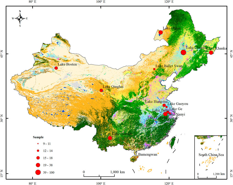
FIGURE 1. Location of lake sites being sampled.

TABLE 1

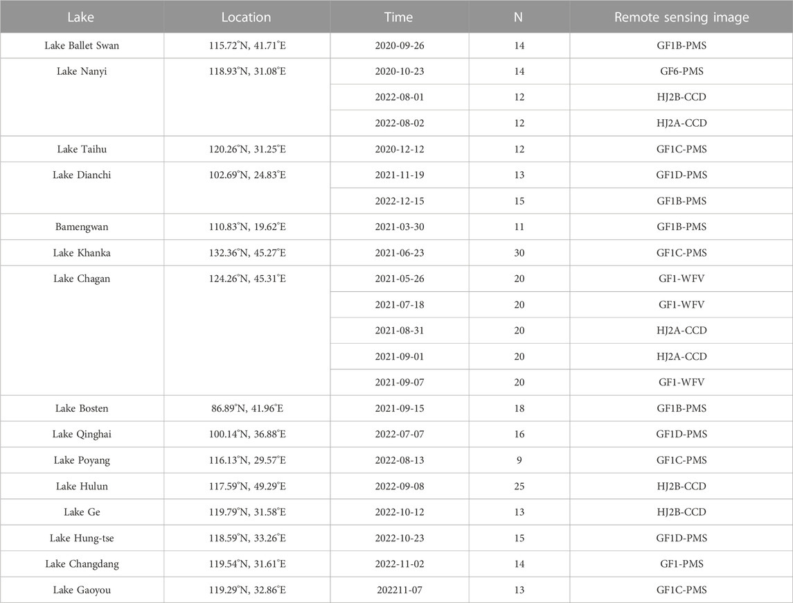
TABLE 1. Name, location, time, sampling number, and satellite synchronous image of lakes across China used in the present study.

2.2 Broad bandwidth satellite

The remote sensing images of broad bandwidth satellites are from the China Centre for Resources Satellite Data and Application (https://data.cresda.cn/). The remote sensing images come from 8 sensors of 7 satellites, including GF1-PMS, GF1-WFV, GF1B-PMS, GF1C-PMS, GF1D-PMS, GF6-PMS, HJ2A-CCD, and HJ2B-CCD. Their band setting is the same: blue/band 1, green/band 2, red/band 3, and near-infrared/band 4, four spectral bands. The spectral response functions of each sensor are highly similar (Figures 2, 3). The networked joint observation of multiple sensors can meet the requirements of daily full-coverage observation of the whole of China, which is suitable for the dynamic monitoring of lakes in China. Twenty-two broad bandwidth remote sensing images matching the field sampling data were downloaded. The time window is within 1 day of the on-site sampling time. The Second Simulation of a Satellite Signal in the Solar Spectrum vector code (6sV) was used to complete the atmospheric correction of each satellite data, which was used in producing remote sensing products for the TSM concentration in lakes.

FIGURE 2

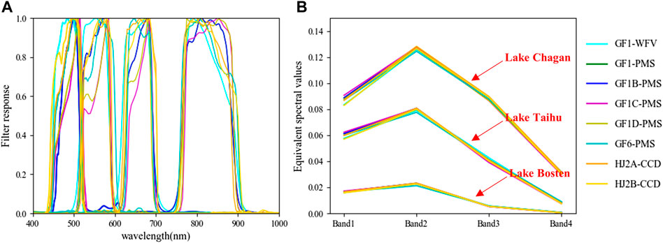
FIGURE 2. The spectral response functions of each sensor (A) and the simulation results of a single spectrum under different spectral response functions (B).

FIGURE 3

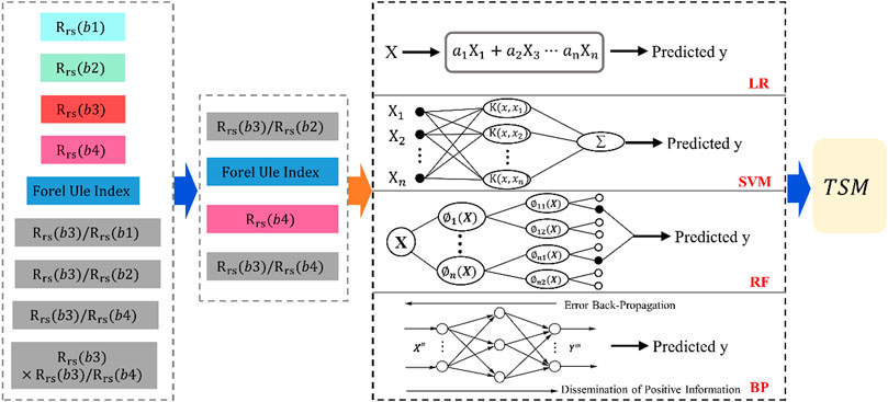
FIGURE 3. Schematic diagram of four machine learning algorithms for optimal TSM retrieve from $R_{rs}\left(\gamma \right)$ combination.

2.3 In Situ data

The in-situ data include the water spectrum data and the TSM concentration data in lakes. The determination of the TSM concentration adopts the laboratory measurement method, and the process of drying, roasting, and weighing is carried out in the laboratory. The water spectral data are measured by the water spectrometer model RAMSES produced by the German TRIOS company, and the measurement method is the water surface measurement method.

The in-situ spectral data of the lakes is equivalent to the water remote sensing reflectance through the integral band operation (Martins et al., 2017). As shown in Formula 1:

$R_{rs}\left({\gamma }_i\right)=\frac{{\sum }_{j=1}^n{F}_i\left({\gamma }_j\right)R_{rs}\left({\gamma }_j\right)}{{\sum }_{j=1}^n{F}_i\left({\gamma }_j\right)}(1)$

Where $R_{rs}\left({\gamma }_i\right)$ (${sr}^{-1}$) is water remote sensing reflectance; $F_i$ is the spectral response function of the $i$ th band of the broadband satellite sensor synchronized with the in-situ data.

The water spectrum data were used to simulate the true values of remote sensing reflectance observed by satellite sensors. Three spectral data of three different TSM concentrations of 6 mg/L, 26 mg/L, and 48 mg/L were selected, and Formula 1 was used to simulate the remote sensing reflectance of eight sensors (Figure 2). Table 2 showed that the MAPE of broad bandwidth satellite remote sensing reflectance under different TSM concentrations was 2.11%, indicating that different broad bandwidth satellites transferred about 2% error in the retrieval model.

TABLE 2

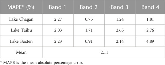
TABLE 2. Simulation accuracy of single spectrum under different spectral response function.

3 Methods

This study compares several representative machine learning algorithms of TSM concentration that are most widely used. To enhance the feature set of the machine learning model, based on the four bands of blue, green, red, and near-infrared, using the band combination of TSM retrieval in the existing literature and FUI (Section 3.1) are considered as the feature variable. These spectral variables are used to estimate the TSM concentration in water to check the performance of the machine-learning model.

3.1 Forel-Ule Index

The FUI is one of the monitoring data of traditional water quality optical properties. The FUI is closely related to changes in water quality parameters and has strong potential and advantages in monitoring water quality on a regional and global long-term scale. Moreover, the FUI extracted from satellite images has higher accuracy and is closely related to the TSM concentration. The remote sensing extraction of the FUI has strong stability and can convert between different sensors (Wernand et al., 2013; Garaba et al., 2015; Li et al., 2016). Based on the Forel-Ule Scale, the color of natural water is divided into 21 color levels, from dark blue to reddish brown (Novoa et al., 2013; Wang et al., 2014). Therefore, The FUI are added to supplement the input feature dataset of the machine learning model. The calculation method of the FUI refers to the research paper of Li et al. (Wang et al., 2021).

3.2 Machine learning model

Machine learning models can automatically identify and capture the characteristics of training data and develop predictive models with good performance (Reichstein et al., 2019). Several representative machine learning models are used in the TSM retrieve in water quality, including linear regression, support vector regression, random forest, and BP neural network. To ensure the accuracy and generalization of the retrieved model, The in-situ data and spectral data were divided into the training dataset (N = 230), validation dataset (N = 100), test dataset (Lake Chagan (2021-08-31), Lake Changdang). Water spectral characteristic variables are used to estimate the TSM concentration to check the performance of the machine learning models.

3.2.1 Linear regression

Linear regression establishes an approximately linear relationship between the independent variable $x_i$ and the dependent variable $y.$ When a dataset n is given, the model can be expressed by Formula 2:

$y={\beta }_0+{\beta }_1{x}_{i1}+\cdots +{\beta }_p{x}_{ip}+{\epsilon }_i=x_i^T\beta +{\epsilon }_i,i=\mathrm{1,2},\cdots ,n(2)$

where $y$ is the dependent variable, ${\beta }_i$ is the polynomial coefficient of $x_i$, $p$ is the number of independent variables, ${\epsilon }_i$ is the $ith$ possible variation, and $x_i^T$ is the inner product between vectors $x_i$ and ${\beta }_i$.

$y=\left(\begin{array}{c}{y}_1\\ \begin{array}{c}{y}_2\\ ⋮\end{array}\\ y_n\end{array}\right),X=\left(\begin{array}{c}{x}_1^T\\ \begin{array}{c}{x}_2^T\\ ⋮\end{array}\\ x_n^T\end{array}\right)=\left(\begin{array}{c}\begin{array}{cc}\begin{array}{ccc}1& x_{11}& \cdots \end{array}& x_{1p}\end{array}\\ \begin{array}{c}\begin{array}{cc}\begin{array}{ccc}1& x_{21}& \cdots \end{array}& x_{2p}\end{array}\\ \begin{array}{cc}\begin{array}{ccc}⋮& ⋮& x_{i,p}\end{array}& ⋮\end{array}\end{array}\\ \begin{array}{cc}\begin{array}{ccc}1& x_{n1}& \cdots \end{array}& x_{np}\end{array}\end{array}\right),\beta =\left(\begin{array}{c}{\beta }_1\\ \begin{array}{c}{\beta }_1\\ ⋮\end{array}\\ {\beta }_n\end{array}\right),\epsilon =\left(\begin{array}{c}{\epsilon }_1\\ \begin{array}{c}{\epsilon }_1\\ ⋮\end{array}\\ {\epsilon }_n\end{array}\right)(3)$

where $y_1$ is the $i$ th dependent variable, $x_{i,p}$ is the value of the $i$ th independent variable in the $p$ th data, based on the classical matrix operation theory, LR model uses the least squares method to solve coefficients of the vector $\beta$ and predict the dependent variable $y$.

3.2.2 Support vector regression

Support Vector Regression aims to present the dataset in a high-dimensional feature space via non-linear mapping and solve the prediction problem. Find a hyperplane with the smallest linear approximation distance to the sample dataset in the feature space. For the training dataset $D=\left\{\left(x_1,y_1\right),\left(x_2,y_2\right)\cdots ,\left(x_m,y_m\right)\right\},y_i\in R$, find a hyperplane given:

$f\left(x\right)=w\varnothing \left(x\right)+b(4)$

where $x$ is an independent variable, $w$ is a weight vector, $\varnothing \left(x\right)$ is a non-linear mapping function, and $b$ is a bias term. The kernel function uses the radial basis function.

3.2.3 Random forest regression

Random Forest Regression is an ensemble learning method that inputs data from random sampling into many weak learners (decision trees) and votes to obtain the final output (Victor et al., 2014). The MSE standard grows a single decision tree, and the predicted target variable is computed as the average prediction of all decision trees. The steps of the RF regression algorithm are as follows: First, apply bootstrap to extract $m$ sample datasets from all training samples with replacement to construct $m$ regression trees, and the unselected samples form $m$ out-of-big datasets. Then, at each tree node, a part of the segmentation variables is randomly selected from all explanatory variables, and the optimal branch is chosen according to the branching goodness criterion. Finally, each regression tree starts recursive branching from top to bottom until the split termination condition is met. The advantages of random forest regression are: that the learning process is fast; for large-scale datasets, it is an efficient processing algorithm, and it has strong robustness to the noise in the dataset.

3.2.4 BP neural network

The back propagation neural network is a feed-forward network proposed by Rumelhart and McClelland, which uses the error back propagation algorithm as the learning rule for supervised learning (Teodoro et al., 2007). By training known samples, find out the relationship between the characteristic attributes of the input samples and the target output. Suppose the number of input nodes of the network is M and the number of output nodes is L. In that case, this neural network can be regarded as an M-dimensional Euclidean space to Mapping of L-dimensional Euclidean spaces. It uses the error back propagation algorithm. The BP neural network is usually composed of an input layer, an output layer, and a hidden layer. The neurons between the layers are fully interconnected. The neurons in each layer are not connected. Interconnected through the corresponding network weight coefficient $w$.

3.3 Statistical analyses and accuracy assessment

The mean absolute percentage error (MAPE), the mean absolute error (MAE), and the root mean square error (RMSE) are used to evaluate the performance of the TSM concentration retrieval model. Their formulas are as follows:

$MAPE=\frac{100\%}{N}{\displaystyle \sum }_{i=1}^N\left|\frac{E_i-M_i}{M_i}\right|(5)$

$MAE=\frac{1}{N}{\displaystyle \sum }_{i=1}^N\left|E_i-M_i\right|(6)$

$RMSE=\sqrt{\frac{1}{N}{\displaystyle \sum }_{i=1}^N{\left(E_i-M_i\right)}^2}(7)$

where $N$ is the total number of data, $i$ represents a single data; $M$ and $E$ are measured values and estimated values, respectively.

4 Results and analysis

4.1 TSM data analysis

Figure 4 showed the change differences in the TSM concentration in each lake. This difference reflected the impact of human life on the water environment of the lake. For example, Qinghai Lake and Lake Bosten were located in the central and western parts of China. Because the lakes are governed and protected by the local government, and the TSM concentration were lower. The highest values of TSM concentration in Lake Chagan and Lake Xingkai were more significant than 100 mg/L. They were located near towns in northern China, so they were highly vulnerable to human activities. The TSM concentration in all samples ranged from 1 to 126 mg/L, averaging 40 mg/L. It showed that our lake dataset contains the $R_{rs}\left({\gamma }_i\right)$ of the lake type of 0–130 mg/L, and did not contain the lakes with high TSM concentration higher than 130 mg/L.

FIGURE 4

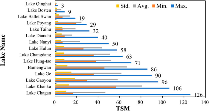
FIGURE 4. Data analysis of suspended solids in each lake.

4.2 Machine learning input feature variable screening

Based on the four bands of blue (Band 1), green (Band 2), red (Band 3), and near-infrared (Band 4), band combinations (Band 3/Band 2, Band 3/Band 1, Band 3/Band 4, Band 2*Band 3/Band 1) and the FUI were used as the feature variables for the TSM concentration retrieve (Du et al., 2020; Liu et al., 2021). However, if there was a strong correlation between the feature variables, it may lead to multicollinearity of the dataset, affecting the solution’s spatial instability. The Mean Decrease Impurity (MDI) feature selection method in Scikit-learn were used to reduce the dimensionality of the feature dataset. The feature importance ranking was shown in Figure 5. Band 3/Band 2 features variables had the highest proportion of importance, which was 0.44. The importance of the top four feature variables accounted for more than 80%. Therefore, the final selected four feature variables, Band 3/Band 2, FUI, Band 4, and Band 3/Band 4, were used to retrieve the TSM concentration.

FIGURE 5

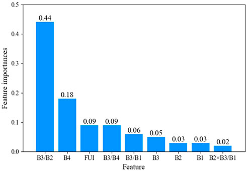
FIGURE 5. Ranking of the importance of feature variables.

4.3 TSM retrieve model calibration and validation

The following comparative analysis on the TSM retrieve model were conducted: evaluated the retrieved model of TSM concentration in the existing documented; compared and evaluated four machine learning methods; considered the influence of FUI on the accuracy of TSM retrieve model.

Six existing documented models were compared in this study (Table 3). Figure 6 showed the retrieval performance of the six models in existing datasets. All TSM concentration retrieve models were generally underestimated at high values. Overestimation occurred in the low-value area. The performance of Model 2 and Model 5 was the most prominent, and their predicted values was concentrated between 20 and −60 mg/L, and they were not sensitive to low and high TSM concentration. Although the fitting coefficients of Model 1, Model 3, and Model 6 were above 0.4, the MAPEs were all above 54%, indicating obvious faults in the shallow value area (<10 mg/L) and other value areas. Therefore, the existing documented models often exhibited high dispersion and error characteristics when targeting different types of lakes and were not suitable for joint retrieve research of TSM concentration in multiple lakes.

TABLE 3

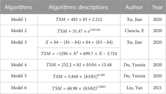
TABLE 3. Documented candidate TSM algorithms related to 4 bands.

FIGURE 6

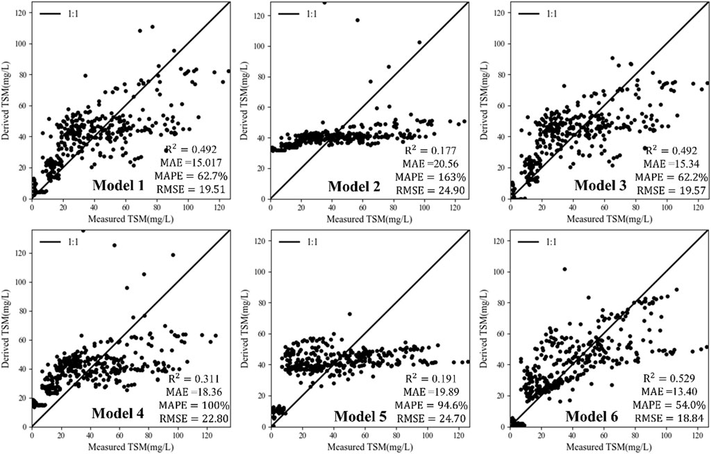
FIGURE 6. Scatter plots of derived and measured values of TSM concentrations according to documented candidate TSM algorithms related to Broad bandwidth satellite (Table 3), The unit of RMSE and MAE mg/L.

Machine learning algorithms had good performance for feature capture of training datasets. The retrieved results of the four machine-learning models were shown in Figure 7 (Table 2). The statistical indicators of the validation dataset showed that among the four machine learning models, the RF model ($R^2=0.83,MAPE=25.5\%$) and BP model ($R^2=0.80,MAPE=22.7\%$) show good performance (slope close to 1) and relatively low error. In contrast, the SVR model ($R^2=0.55,MAPE=114.4\%$) algorithm showed good learning performance in the low-value area, but underestimated the TSM concentration (>50 mg/L) in the high-value area, the results of LR model ($R^2=0.59,MAPE=94.3\%$) also showed that the high-value area was underestimated, and its dispersion was high. Therefore, we considered the RF and BP models as candidate models for the TSM retrieval model.

FIGURE 7

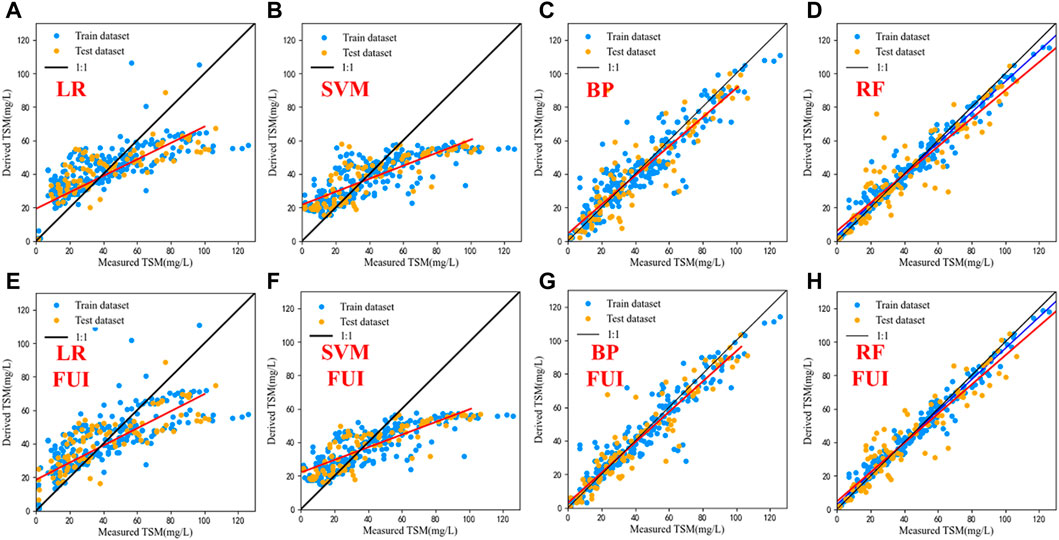
FIGURE 7. (B, D, F, H) were the training and validation accuracy of the four machine learning models without FUI, and (A, C, E, G) were the training and validation accuracy of four machine learning models with FUI.

The FUI divided water bodies into different categories, covering an extensive range of natural water optical features. The FUI was added into the machine learning model. Figures 7E, F, G, H) showed the accuracy changes of the four machine learning models after adding the FUI. The MAE of the four machine learning models on the test dataset was reduced from 16.06 mg/L, 15.30 mg/L, 8.06 mg/L, and 7.52 mg/L to 15.14 mg/L, 15.21 mg/L, 6.69 mg/L, 6.92 mg/L (Table 4). At the same time, RMSE decreased by an average of 1.48 mg/L among the four models. By comparing the RF model (Figures 7D, H), it was found that in the TSM concentration of 30–50 mg/L, the FUI effectively captured the change characteristics, which significantly improved the performance of the model on the validation dataset. Figures 7G, H showed that the FUI can make the machine learning model converge better and improve the training accuracy of the BP model and RF model ($\mathrm{R}\mathrm{F}:R^2=0.97,BP:R^2=0.91$) and Validation accuracy ($\mathrm{R}\mathrm{F}:R^2=0.88,BP:R^2=0.88$). The resulted showed that the FUI could improve the accuracy of the TSM retrieval model in the machine-learning model.

TABLE 4

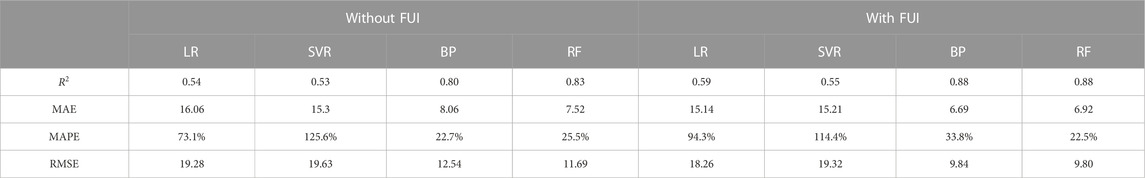
TABLE 4. Accuracy evaluation of four machine learning models.

4.4 TSM retrieve model generalization

The RF model and BP model were used to retrieve the TSM concentration in Lake Chagan (2021-8-31) and Lake Changdang (Figure 8). The Lake Chagan dataset was used to verify the generalization ability of the TSM model for the machine learning model in different phases of the same lake. The Lake Changdang dataset was used to demonstrate the generalization ability of machine learning in different lakes and time phases. The resulted showed that the prediction model of the RF model and BP model had the best performance in Lake Chagan ($\mathrm{R}\mathrm{F}:R^2=0.935,BP:R^2=0.885$) and Lake Changdang ($\mathrm{R}\mathrm{F}:R^2=0.898,BP:R^2=0.752$) showed good performance. But the RF model was superior to the BP model in the statistical indicators of MAPE and RMSE. And the MAE of the RF model was less than 2 mg/L, which showed that compared with the BP model, the RF model had a better generalization ability, and its prediction results of TSM concentration could be effectively guaranteed.

FIGURE 8

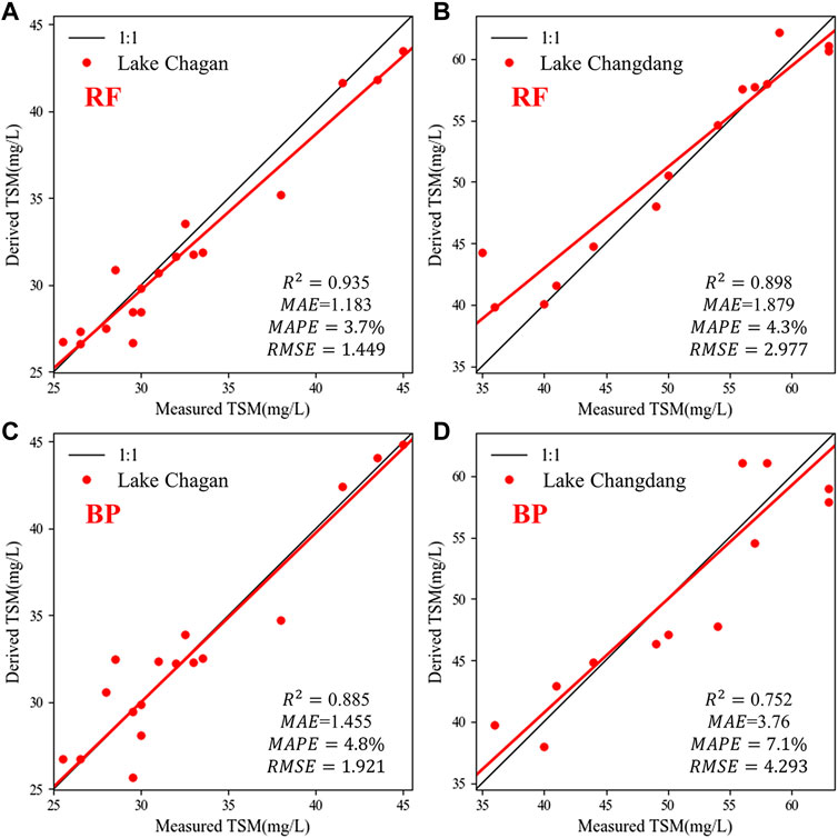
FIGURE 8. Generalization ability of RF retrieve model and BP retrieve model. RF model (A, B) and BP model (C, D).

4.5 Spatial variations of TSM with broad bandwidth satellite: Examples

The RF model was used to retrieve the TSM concentration in Lake Bosten, Lake Chagan, and Lake Changdang in this study. Lake Bosten was used to verify the retrieval accuracy of the TSM concentration used for modeling. Lake Chagan and Lake Changdang were to prove the generalization performance of the RF model. The remote sensing images of the three lakes used were the HJ2A-CCD image on 31 August 2021, the GF1B-PMS image on 15 September 2021, and the GF1-PMS image on 2 November 2022. The imaging time of the remote sensing image and the on-site sampling time were both carried out on the same day, and the verification validity of the in-situ data could be guaranteed. Figures 9A–C showed the validation results of retrieving TSM concentrations in three lakes. The MAPEs of the three lakes were 5.3%, 8.1%, and 12.1%, respectively, and the results reached relatively high precision. Compared with the retrieved results of the water spectra data of Lake Chagan and Lake Changdang (Figures 8A, B), the retrieval accuracy of remote sensing images needed to be higher. The reason may be that the accuracy error images of radiometric and atmospheric correction models limited remote sensing images. There was a certain error between the remote-sensing spectrum data and the in-situ spectrum data. For example, the retrieve of TSM concentration in Lake Changdang had an overestimation (>10 mg/L) in the high-value area (60–75 mg/L). At the same time, the in-situ spectral data of (Figure 8B) could better invert the high-value area of TSM concentration. Lake Bosten was the largest freshwater lake in China. The water quality environment had always been good, and the TSM concentration was deficient (0–15 mg/L). The TSM concentration in Lake Chagan and Lake Changdang was relatively high (33–89 mg/L, 32–84 mg/L). The reason may be that the two lakes are located on the edge of the city and are greatly affected by human activities such as agriculture and industry.

FIGURE 9

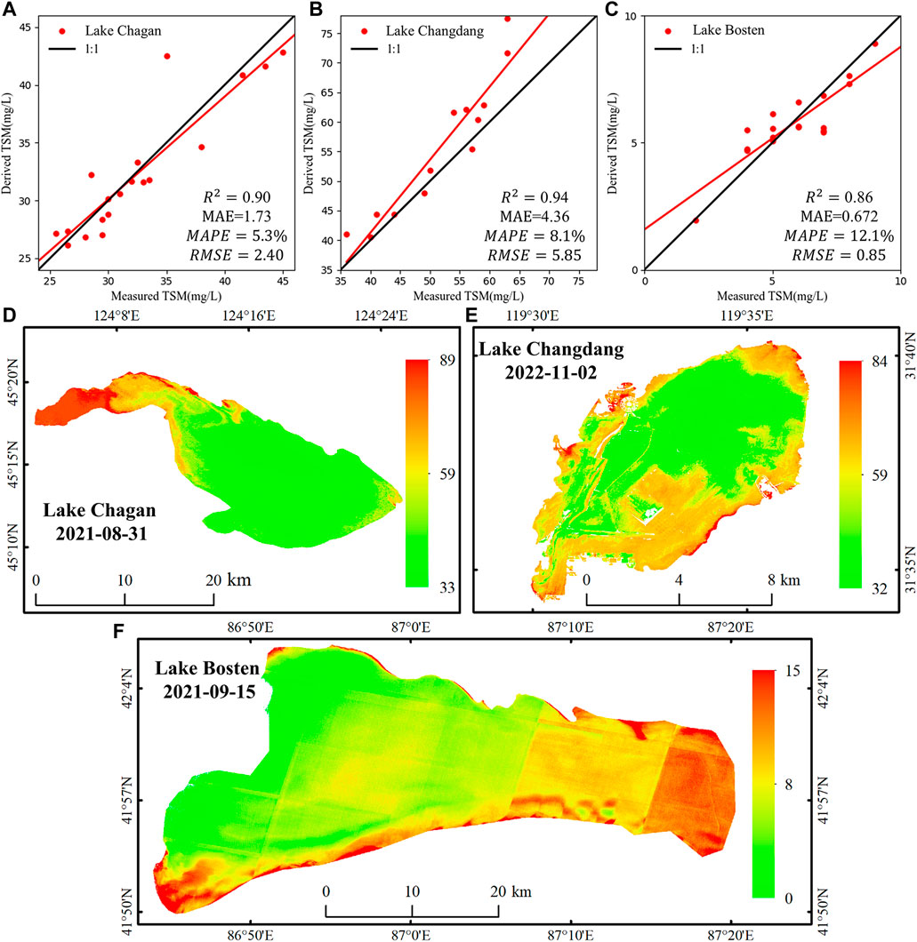
FIGURE 9. The generalization ability of RF Retrieve model, Lake Chagan (A, D), Lake Changdang (B, E), and Lake Bosten (C, F).

5 Discussion

Satellite remote sensing images provide an effective observation method for estimating the TSM concentration in large-scale and long-term series. The accuracy of the retrieved model directly affects the reliability of the retrieved results. Currently, the research on the retrieved model for the TSM concentration mainly focuses on the retrieved model of a single lake or a single sensor. However, the spatial coverage capability and revisit period of a single sensor are limited by orbital parameters, and achieving the dynamic monitoring requirements of TSM concentration is difficult. Therefore, the collaborative retrieval of multiple sensors is required to improve the dynamic monitoring of TSM concentration. On the other hand, the documented research results showed that RF model has excellent performance in the TSM retrieve of regional lakes (Shen et al., 2020; Wang et al., 2022b; Xu et al., 2022). The advantage of RF model is that the learning process is fast; It is an efficient processing model for large datasets. And it has strong robustness to noise in dataset (Shen et al., 2022). Therefore, A random forest-based machine learning model was developed to solve the applicability of multi-source broad bandwidth satellite data collaborative retrieval of regional typical TSM concentrations in this study. The retrieved results of three different types of lakes (Lake Bosten, Lake Chagan, and Lake Changdang) showed that the RF model has high accuracy (MAPE<15%). These studies showed that the RF model could effectively solve the problem of the applicability of the broad bandwidth satellites retrieval of TSM concentration and meet the accuracy requirements of large-scale and dynamic monitoring of lakes.

5.1 Application limitations

The RF model proposed in this study preliminarily solves the applicability of broad bandwidth satellites to retrieve the TSM concentration in different types of water. But the RF model also has certain limitations. First, the machine learning model requires a large amount of in-situ data, enabling it to capture the water spectral features of various TSM concentrations. The ideal training data should collect long-term continuous water spectrum and TSM concentration data in various typical lakes in China so that the spectral characteristics of these types of lakes can fully characterize the changes in TSM concentration. However, the acquisition cost of these data is relatively high in actual work. Therefore, 22 water experiment data from 15 lakes were selected as the dataset in this sutdy. There is a certain need for more training data. The range of TSM concentration can only cover the range of 0–120 mg/L, and there is a lack of training data for highly turbid water (TSM>10 0 mg/L). This makes the RF model proposed has a better retrieve effect for water bodies with medium and low suspended solids concentrations. Still, the accuracy must be verified more in high turbid water bodies. Secondly, this study is the first attempt to use a combination of multiple broad bandwidth satellites to retrieve the TSM. The true value of remote sensing reflectance of each broad bandwidth satellite is calculated by Formula 5. However, although the bands of these broad bandwidth satellites are similar, there are certain differences in the sensitivity of their sensors to different bands. This results in a certain error ($MAPE\approx 2\%$) when the true value of the reflectance formed corresponds to different satellites after spectral equivalence. Using the equivalent true data of these different satellites to carry out unified modeling research will increase the uncertainty of the TSM retrieved model to a certain extent. The evaluation of this uncertainty still needs to be verified through continuous experiments.

5.2 Future plan

This study attempts to use various broad bandwidth satellites to carry out comprehensive TSM concentration retrieval. The purpose is to develop a TSM retrieve model compatible with various high-resolution broad bandwidth satellites to meet the requirements of water dynamic monitoring. RF and various neural network models have good model generalization ability, and the quality of the accuracy of the TSM retrieve model is primarily affected by the amount of data. The RF model proposed is to obtain the optimal model in the existing dataset. In the future research, on the one hand, the research team will continue to accumulate water quality data of typical lakes in China, the model will continue to iterate and update. We will continue to optimize the model to obtain a broad bandwidth satellite TSM retrieve model with better stability and accuracy. On the other hand, the bandwidth and spectrum of broad bandwidth satellite sensors are very similar. Therefore, we consider building these satellites into virtual constellations, carry out research on the normalization of remote sensing spectra of broadband satellites, and eliminate observation errors between different sensors. The coordinated operation among satellites can meet the demand of regional lakes dynamic observation.

6 Conclusion

TSM concentrations have spatial-temporal heterogeneity in different lakes. To meet the dynamic monitoring requirements of TSM concentration, machine learning models have potential applicability in TSM retrieval. The accuracy and relevance of the four machine learning models of the LR model, SVR model, RF model and BP model are tested through the in-situ datasets of multiple lakes. Compared with other machine learning models, the RF model provided better performance. The RF model has good generalization ability, showing high verification accuracy in both validation datasets and practical applications. The FUI can effectively enhance the precision and accuracy of the TSM retrieve model. Therefore, this study showed that the RF model can improve the retrieve performance and generalization ability of the broad bandwidth satellite’s TSM concentration in lakes and meet the accuracy requirements of high-frequency and dynamic monitoring of TSM concentration. With the continuous accumulation of more in-situ lake data, the accuracy and stability of the TSM retrieve model proposed in this study will be further improved.

Data availability statement

The raw data supporting the conclusion of this article will be made available by the authors, without undue reservation.

Author contributions

MZ: Conceptualization, methodology, and writing-original draft and editing; ZT: Conceptualization, formal analysis, validation and writing-review; XZ: Supervision and investigation; TL: Writing—review and editing and project administration; HZ: Visualization; RL: Writing—review and editing; YH: Software.

Funding

This work was supported by the National Key R&D Program of China (2018YFE0124200) and The Common Application Support Platform for Land Observation Satellites of China’s Civil Space Infrastructure.

Acknowledgments

We would like to thank the reviewers for their constructive suggestions and comments.

Conflict of interest

The authors declare that the research was conducted in the absence of any commercial or financial relationships that could be construed as a potential conflict of interest.

Publisher’s note

All claims expressed in this article are solely those of the authors and do not necessarily represent those of their affiliated organizations, or those of the publisher, the editors and the reviewers. Any product that may be evaluated in this article, or claim that may be made by its manufacturer, is not guaranteed or endorsed by the publisher.

References

Aires, F., Venot, J.-P., Massuel, S., Gratiot, N., Pham-Duc, B., and Prigent, C. (2020). Surface water evolution (2001–2017) at the Cambodia/Vietnam border in the upper mekong delta using satellite MODIS observations. Remote Sens. 12, 800. doi:10.3390/rs12050800

CrossRef Full Text | Google Scholar

Ali, K. A., and Ortiz, J. D. (2016). Multivariate approach for chlorophyll-a and suspended matter retrievals in Case II type waters using hyperspectral data. Hydrological Sci. J. 61, 200–213. doi:10.1080/02626667.2014.964242

CrossRef Full Text | Google Scholar

Bilotta, G. S., and Brazier, R. E. (2008). Understanding the influence of suspended solids on water quality and aquatic biota. Water Res. 42, 2849–2861. doi:10.1016/j.watres.2008.03.018

PubMed Abstract | CrossRef Full Text | Google Scholar

Bonansea, M., Ledesma, M., Rodriguez, C., and Pinotti, L. (2019). Using new remote sensing satellites for assessing water quality in a reservoir. Hydrological Sci. J. 64, 34–44. doi:10.1080/02626667.2018.1552001

CrossRef Full Text | Google Scholar

Cao, Z., Duan, H., Feng, L., Ma, R., and Xue, K. (2017). Climate-and human-induced changes in suspended particulate matter over Lake Hongze on short and long timescales. Remote Sens. Environ. 192, 98–113. doi:10.1016/j.rse.2017.02.007

CrossRef Full Text | Google Scholar

Chen, J., Quan, W., Cui, T., and Song, Q. (2015). Estimation of total suspended matter concentration from MODIS data using a neural network model in the China eastern coastal zone. Estuar. Coast. Shelf Sci. 155, 104–113. doi:10.1016/j.ecss.2015.01.018

CrossRef Full Text | Google Scholar

Chen, L., Letu, H., Fan, M., Shang, H., Tao, J., Wu, L., et al. (2022). An introduction to the Chinese high-resolution earth observation system: Gaofen-1∼ 7 civilian satellites. J. Remote Sens. 2022, 2022. doi:10.34133/2022/9769536

CrossRef Full Text | Google Scholar

Ciancia, E., Campanelli, A., Lacava, T., Palombo, A., Pascucci, S., Pergola, N., et al. (2020). Modeling and multi-temporal characterization of total suspended matter by the combined use of Sentinel 2-MSI and Landsat 8-OLI data: The pertusillo lake case study (Italy). Remote Sens. 12, 2147. doi:10.3390/rs12132147

CrossRef Full Text | Google Scholar

Dörnhöfer, K., and Oppelt, N. (2016). Remote sensing for lake research and monitoring–Recent advances. Ecol. Indic. 64, 105–122. doi:10.1016/j.ecolind.2015.12.009

CrossRef Full Text | Google Scholar

Doxaran, D., Lamquin, N., Park, Y.-J., Mazeran, C., Ryu, J.-H., Wang, M., et al. (2014). Retrieval of the seawater reflectance for suspended solids monitoring in the East China Sea using MODIS, MERIS and GOCI satellite data. Remote Sens. Environ. 146, 36–48. doi:10.1016/j.rse.2013.06.020

CrossRef Full Text | Google Scholar

Du, Y., Song, K., Liu, G., Wen, Z., Fang, C., Shang, Y., et al. (2020). Quantifying total suspended matter (TSM) in waters using Landsat images during 1984–2018 across the Songnen Plain, Northeast China. J. Environ. Manag. 262, 110334. doi:10.1016/j.jenvman.2020.110334

CrossRef Full Text | Google Scholar

Eleveld, M. A., Pasterkamp, R., van der Woerd, H. J., and Pietrzak, J. D. (2008). Remotely sensed seasonality in the spatial distribution of sea-surface suspended particulate matter in the southern North Sea. Estuar. Coast. Shelf Sci. 80, 103–113. doi:10.1016/j.ecss.2008.07.015

CrossRef Full Text | Google Scholar

Garaba, S. P., Friedrichs, A., Voß, D., Zielinski, O., and health, p. (2015). Classifying natural waters with the forel-ule colour index system: Results, applications, correlations and crowdsourcing. Int. J. Environ. Res. Public Health 12, 16096–16109. doi:10.3390/ijerph121215044

PubMed Abstract | CrossRef Full Text | Google Scholar

Gernez, P., Barillé, L., Lerouxel, A., Mazeran, C., Lucas, A., and Doxaran, D. (2014). Remote sensing of suspended particulate matter in turbid oyster-farming ecosystems. J. Geophys. Res. Oceans 119, 7277–7294. doi:10.1002/2014jc010055

CrossRef Full Text | Google Scholar

Guo, Q., Wu, H., Jin, H., Yang, G., and Wu, X. (2022). Remote sensing inversion of suspended matter concentration using a neural network model optimized by the partial least squares and particle swarm optimization algorithms. Sustainability 14, 2221. doi:10.3390/su14042221

CrossRef Full Text | Google Scholar

Ho, J. C., Michalak, A. M., and Pahlevan, N. (2019). Widespread global increase in intense lake phytoplankton blooms since the 1980s. Nature 574, 667–670. doi:10.1038/s41586-019-1648-7

PubMed Abstract | CrossRef Full Text | Google Scholar

Konik, M., Kowalczuk, P., Zabłocka, M., Makarewicz, A., Meler, J., Zdun, A., et al. (2020). Empirical relationships between remote-sensing reflectance and selected inherent optical properties in Nordic Sea surface waters for the MODIS and OLCI ocean colour sensors. Remote Sens. 12, 2774. doi:10.3390/rs12172774

CrossRef Full Text | Google Scholar

Leong, W. C., Bahadori, A., Zhang, J., and Ahmad, Z. (2021). Prediction of water quality index (WQI) using support vector machine (SVM) and least square-support vector machine (LS-SVM). Int. J. River Basin Manag. 19, 149–156. doi:10.1080/15715124.2019.1628030

CrossRef Full Text | Google Scholar

Li, J., and Roy, D. P. (2017). A global analysis of Sentinel-2A, Sentinel-2B and Landsat-8 data revisit intervals and implications for terrestrial monitoring. Remote Sens. 9, 902. doi:10.3390/rs9090902

CrossRef Full Text | Google Scholar

Li, J., Wang, S., Wu, Y., Zhang, B., Chen, X., Zhang, F., et al. (2016). MODIS observations of water color of the largest 10 lakes in China between 2000 and 2012. Int. J. digital earth 9, 788–805. doi:10.1080/17538947.2016.1139637

CrossRef Full Text | Google Scholar

Liu, Y.-M., Zhang, L., Zhou, M., Liang, J., Wang, Y., Sun, L., et al. (2022). A neural networks based method for suspended sediment concentration retrieval from GF-5 hyperspectral images. 红外与毫米波学报, 41.

Google Scholar

Liu, Y., Fan, J.-P., and Jiang, H. (2021). Evaluation of parametric and nonparametric algorithms for the estimation of suspended particulate matter in turbid water using gaofen-1 wide field-of-view sensors. J. Indian Soc. Remote Sens. 49, 2673–2687. doi:10.1007/s12524-021-01405-7

CrossRef Full Text | Google Scholar

Martins, V. S., Barbosa, C. C. F., De Carvalho, L. A. S., Jorge, D. S. F., Lobo, F. D. L., and Novo, E. M. L. D. M. (2017). Assessment of atmospheric correction methods for Sentinel-2 MSI images applied to Amazon floodplain lakes. Remote Sens. 9, 322. doi:10.3390/rs9040322

CrossRef Full Text | Google Scholar

Miller, R. L., and McKee, B. A. (2004). Using MODIS Terra 250 m imagery to map concentrations of total suspended matter in coastal waters. Remote Sens. Environ. 93, 259–266. doi:10.1016/j.rse.2004.07.012

CrossRef Full Text | Google Scholar

Nechad, B., Ruddick, K. G., and Park, Y. (2010). Calibration and validation of a generic multisensor algorithm for mapping of total suspended matter in turbid waters. Remote Sens. Environ. 114, 854–866. doi:10.1016/j.rse.2009.11.022

CrossRef Full Text | Google Scholar

Novoa, S., Wernand, M., and Van der Woerd, H. (2013). The forel-ule scale revisited spectrally: Preparation protocol, transmission measurements and chromaticity. J. Eur. Opt. Society-Rapid Publ. 8, 13057. doi:10.2971/jeos.2013.13057

CrossRef Full Text | Google Scholar

Ouillon, S., Douillet, P., Petrenko, A., Neveux, J., Dupouy, C., Froidefond, J.-M., et al. (2008). Optical algorithms at satellite wavelengths for total suspended matter in tropical coastal waters. Sensors 8, 4165–4185. doi:10.3390/s8074165

PubMed Abstract | CrossRef Full Text | Google Scholar

Pahlevan, N., Smith, B., Schalles, J., Binding, C., Cao, Z., Ma, R., et al. (2020). Seamless retrievals of chlorophyll-a from sentinel-2 (msi) and sentinel-3 (OLCI) in inland and coastal waters: A machine-learning approach. Remote Sens. Environ. 240, 111604. doi:10.1016/j.rse.2019.111604

CrossRef Full Text | Google Scholar

Pyo, J., Duan, H., Baek, S., Kim, M. S., Jeon, T., Kwon, Y. S., et al. (2019). A convolutional neural network regression for quantifying cyanobacteria using hyperspectral imagery. Remote Sens. Environ. 233, 111350. doi:10.1016/j.rse.2019.111350

CrossRef Full Text | Google Scholar

Reichstein, M., Camps-Valls, G., Stevens, B., Jung, M., Denzler, J., Carvalhais, N., et al. (2019). Deep learning and process understanding for data-driven Earth system science. Nature 566, 195–204. doi:10.1038/s41586-019-0912-1

PubMed Abstract | CrossRef Full Text | Google Scholar

Saberioon, M., Brom, J., Nedbal, V., Souc̆ek, P., and Císar̆, P. (2020). Chlorophyll-a and total suspended solids retrieval and mapping using Sentinel-2A and machine learning for inland waters. Ecol. Indic. 113, 106236. doi:10.1016/j.ecolind.2020.106236

CrossRef Full Text | Google Scholar

Shen, M., Duan, H., Cao, Z., Xue, K., Qi, T., Ma, J., et al. (2020). Sentinel-3 OLCI observations of water clarity in large lakes in eastern China: Implications for SDG 6.3. 2 evaluation. Remote Sens. Environ. 247, 111950. doi:10.1016/j.rse.2020.111950

CrossRef Full Text | Google Scholar

Shen, M., Luo, J., Cao, Z., Xue, K., Qi, T., Ma, J., et al. (2022). Random forest: An optimal chlorophyll-a algorithm for optically complex inland water suffering atmospheric correction uncertainties. J. Hydrology 615, 128685. doi:10.1016/j.jhydrol.2022.128685

CrossRef Full Text | Google Scholar

Siswanto, E., Tang, J., Yamaguchi, H., Ahn, Y.-H., Ishizaka, J., Yoo, S., et al. (2011). Empirical ocean-color algorithms to retrieve chlorophyll-a, total suspended matter, and colored dissolved organic matter absorption coefficient in the Yellow and East China Seas. J. Oceanogr. 67, 627–650. doi:10.1007/s10872-011-0062-z

CrossRef Full Text | Google Scholar

Tan, Z., Cao, Z., Shen, M., Chen, J., Song, Q., and Duan, H. (2022). Remote estimation of water clarity and suspended particulate matter in qinghai lake from 2001 to 2020 using MODIS images. Remote Sens. 14, 3094. doi:10.3390/rs14133094

CrossRef Full Text | Google Scholar

Teodoro, A. C., Veloso-Gomes, F., and Goncalves, H. (2007). Retrieving TSM concentration from multispectral satellite data by multiple regression and artificial neural networks. IEEE Trans. Geoscience Remote Sens. 45, 1342–1350. doi:10.1109/tgrs.2007.893566

CrossRef Full Text | Google Scholar

Uddin, S., Al-Ghadban, A., Gevao, B., Al-Shamroukh, D., and Al-Khabbaz, A. (2012). Estimation of suspended particulate matter in Gulf using MODIS data. Aquat. Ecosyst. Health Manag. 15, 41–44. doi:10.1080/14634988.2012.668114

CrossRef Full Text | Google Scholar

Victor, R. G., Maria Jose, G-S., Mario, C-O., Luis, R., and Ribeiro, L., Predictive modeling of groundwater nitrate pollution using random forest and multisource variables related to intrinsic and specific vulnerability: A case study in an agricultural setting (southern Spain). Sci. Total Environ. 2014, 476-477, 189–206. doi:10.1016/j.scitotenv.2014.01.001

PubMed Abstract | CrossRef Full Text | Google Scholar

Wang, S., Li, J., Shen, Q., Zhang, B., Zhang, F., and Lu, Z. (2014). MODIS-based radiometric color extraction and classification of inland water with the forel-ule scale: A case study of Lake taihu. IEEE J. Sel. Top. Appl. Earth Observations Remote Sens. 8, 907–918. doi:10.1109/jstars.2014.2360564

CrossRef Full Text | Google Scholar

Wang, S., Li, J., Zhang, W., Cao, C., Zhang, F., Shen, Q., et al. (2021). A dataset of remote-sensed Forel-Ule Index for global inland waters during 2000–2018. Sci. Data 8, 26–10. doi:10.1038/s41597-021-00807-z

PubMed Abstract | CrossRef Full Text | Google Scholar

Wang, X., Song, K., Liu, G., Wen, Z., Shang, Y., and Du, J. (2022). Development of total suspended matter prediction in waters using fractional-order derivative spectra. J. Environ. Manag. 302, 113958. doi:10.1016/j.jenvman.2021.113958

CrossRef Full Text | Google Scholar

Wang, X., Wen, Z., Liu, G., Tao, H., and Song, K. (2022). Remote estimates of total suspended matter in China’s main estuaries using Landsat images and a weight random forest model. ISPRS J. Photogrammetry Remote Sens. 183, 94–110. doi:10.1016/j.isprsjprs.2021.11.001

CrossRef Full Text | Google Scholar

Wang, X., and Xie, H. (2018). A review on applications of remote sensing and geographic information systems (GIS) in water resources and flood risk management. Water 10, 608. doi:10.3390/w10050608

CrossRef Full Text | Google Scholar

Wernand, M., Hommersom, A., and van der Woerd, H. J. (2013). MERIS-based ocean colour classification with the discrete Forel–Ule scale. Ocean Sci. 9, 477–487. doi:10.5194/os-9-477-2013

CrossRef Full Text | Google Scholar

Xi, H., and Zhang, Y. (2011). Total suspended matter observation in the Pearl River estuary from in situ and MERIS data. Environ. Monit. Assess. 177, 563–574. doi:10.1007/s10661-010-1657-3

PubMed Abstract | CrossRef Full Text | Google Scholar

Xing, Q., Lou, M., Chen, C., and Shi, P. (2013). Using in situ and satellite hyperspectral data to estimate the surface suspended sediments concentrations in the Pearl River estuary. IEEE J. Sel. Top. Appl. Earth Observations Remote Sens. 6, 731–738. doi:10.1109/jstars.2013.2238659

CrossRef Full Text | Google Scholar

Xu, J., Gao, C., and Wang, Y. (2020). Extraction of spatial and temporal patterns of concentrations of chlorophyll-a and total suspended matter in Poyang Lake using GF-1 satellite data. Remote Sens. 12, 622. doi:10.3390/rs12040622

CrossRef Full Text | Google Scholar

Xu, S., Li, S., Tao, Z., Song, K., Wen, Z., Li, Y., et al. (2022). Remote sensing of chlorophyll-a in xinkai lake using machine learning and GF-6 WFV images. Remote Sens. 14, 5136. doi:10.3390/rs14205136

CrossRef Full Text | Google Scholar

Zeng, S., Li, Y., Lyu, H., Xu, J., Dong, X., Wang, R., et al. (2020). Mapping spatio-temporal dynamics of main water parameters and understanding their relationships with driving factors using GF-1 images in a clear reservoir. Environ. Sci. Pollut. Res. 27, 33929–33950. doi:10.1007/s11356-020-09687-z

CrossRef Full Text | Google Scholar

Zhang, B., Li, J., Shen, Q., and Chen, D. (2008). A bio-optical model based method of estimating total suspended matter of Lake Taihu from near-infrared remote sensing reflectance. Environ. Monit. Assess. 145, 339–347. doi:10.1007/s10661-007-0043-2

PubMed Abstract | CrossRef Full Text | Google Scholar

Zhang, C., Liu, Y., Chen, X., and Gao, Y. (2022). Estimation of suspended sediment concentration in the yangtze main stream based on sentinel-2 MSI data. Remote Sens. 14, 4446. doi:10.3390/rs14184446

CrossRef Full Text | Google Scholar

Zhang, G., Yao, T., Chen, W., Zheng, G., Shum, C., Yang, K., et al. (2019). Regional differences of lake evolution across China during 1960s–2015 and its natural and anthropogenic causes. Remote Sens. Environ. 221, 386–404. doi:10.1016/j.rse.2018.11.038

CrossRef Full Text | Google Scholar

Zhang, Y., Shi, K., Liu, X., Zhou, Y., and Qin, B. (2014). Lake topography and wind waves determining seasonal-spatial dynamics of total suspended matter in turbid lake taihu, China: Assessment using long-term high-resolution MERIS data. PloS one 9, e98055. doi:10.1371/journal.pone.0098055

PubMed Abstract | CrossRef Full Text | Google Scholar

Zheng, Z., Li, Y., Guo, Y., Xu, Y., Liu, G., and Du, C. (2015). Landsat-based long-term monitoring of total suspended matter concentration pattern change in the wet season for Dongting Lake, China. Remote Sens. 7, 13975–13999. doi:10.3390/rs71013975

CrossRef Full Text | Google Scholar