Dryness–Wetness Encounter Probabilities’ Analysis for Lake Ecological Water Replenishment Considering Non-Stationarity Effects

Ecological water replenishment (EWR) via interbasin water transfer projects has been regarded as a critical solution to reducing the risk of lake shrinkage and wetland degradation. The hydrological conditions of EWR water sources do not change synchronously, which may have an impact on the transferable water. Based on the GAMLSS model and the multivariate Copula model, this work presents a research approach for EWR via interbasin water transfer projects that can capture the non-stationarity of the runoff series and the frequency of dryness–wetness encounters, as well as speculates on various scenarios throughout the project operation phase. We present a case study on the Baiyangdian Lake, acting as the largest freshwater wetland in North China, which has suffered from severe degradation during the past decades and deserves thorough ecological restoration. The GAMLSS model was used to examine the non-stationarity characteristics of EWR water sources including the Danjiangkou Reservoir (DJK), the Huayuankou reach of the Yellow River (HYK), and upstream reservoirs (UR). The multivariate Copula model was implemented to evaluate the synchronous–asynchronous characteristics for hydrological probabilities for the multiple water sources. Results show that 1) significant non-stationarity has been detected for all water sources. Particularly, a significant decreasing trend has been found in UR and HYK. 2) The non-stationary model with time as the explanatory variable is more suitable for the runoff series of DJK, HYK, and UR. Under the non-stationary framework, the wet–dry classification of runoff series is completely changed. 3) Whether the bivariate or trivariate combination types, the asynchronous probability among the three water resources is over 0.6 except DJK-HYK, which indicates the complementary relationship. Multiple water resources are necessary for EWR. What is more, during a dry year of UR, the conditional probability that both DJK and HYK are in a dry year is 0.234. To alleviate the problem of not having enough water, some additional water resources and an acceptable EWR plan are required.

Introduction

With the rapid increase in the human population and social progress, development has generated significant economic and social benefits, but these benefits often come at high costs. The overexploitation of freshwater resources threatens the ecological environment and the overall well-being of humankind in many parts of the world (Kummu et al., 2016). At present, there are a large number of lakes shrinking and wetlands degrading around the world (Acreman et al., 2007; Chen et al., 2013; Mei et al., 2015; Liu et al., 2019; Ussenaliyeva and Aizhan, 2020; Jones and Fleck, 2020; Stone, 2021). In China, for example, 60.0% of lakes and 28.0% of marshes were threatened by the overuse of water resources, while 43.3% of lakes were threatened by sediments (Wang et al., 2012). Several wetland restoration measures, such as ecological water replenishment, restoring natural waterways, recreating the natural river, establishing habitats, and returning cropland to wetland, are recognized (Xin, 2014; Wu et al., 2020). Among these measures, the ecological water replenishment (EWR) has been widely applied in restoring ecology and hydrological conditions across various climatic and geophysical regions (Onuoha, 2008; Weigang et al., 2018), such as the Baiyangdian wetland (Ding et al., 2019), the Boluo Lake (Huang et al., 2021), and the Chagan Lake (Zhang et al., 2017). Understanding the hydrological synchronization of numerous water sources is critical for the EWR, as the EWR measures are heavily reliant on the hydrological conditions of water sources. The water source area and intake area are usually geographically far apart, which leads to the temporal variation of runoff in the water source area and the intake area being not always synchronous. The asynchrony of the hydrological conditions bears directly on the transferable water quantity and the elapsed time for the water replenishment project. Furthermore, when water sources for EWR become diverse, the hydrological conditions of the water sources can hardly have a consistent change and made the EWR more complicated. Hence, a comprehensive analysis on the hydrological conditions of multiple water sources is suggested in aiding the formation of water diversion schemes (Zhang et al., 2017; Yan et al., 2018).

The basic assumption of traditional hydrological frequency analysis is the assumption of stationarity (Du et al., 2015). However, hydrological series might become non-stationary due to changing climate and underlying surfaces, which leads to the invalidity of the results of hydrological frequency analysis (Lu et al., 2013; Jiang et al., 2015). Therefore, the frequency analysis of non-stationary hydrological series becomes a research focus in the past 20 years. The non-stationarity correction method (Ping et al., 2009) and the time-varying moment method (Strupczewski et al., 2001; Strupczewski and Kaczmarek, 2001) are widely used methods of non-stationary hydrological frequency analysis. The non-stationarity correction method attempted to accurately detect and decompose the abrupt and trend changes in hydrological time series and then compose these components (Xie et al., 2018a; 2018b). The time-varying moment method assumes that hydrologic variables follow some distributions, including GEV and GAMLSS, in which one or more parameters are allowed to vary in time to reflect the non-stationarities of the hydrological series. One of the commonly used tools to examine the hydrological non-stationarity is the GAMLSS model (Jiang et al., 2015; Ahn and Palmer, 2016; Li et al., 2018). GAMLSS was proposed for fitting regression type models, where the distribution of the response variable does not have to belong to the exponential family, and includes highly skew, kurtotic continuous and discrete distribution (Rigby and Stasinopoulos, 2005). GAMLSS allows all the parameters of the distribution of the response variable to be modeled as linear/non-linear or smooth functions of the explanatory variables (Stasinopoulos and Rigby, 2007). Because of these advantages, GAMLSS is widely used in the non-stationary hydrological frequency analysis (Villarini et al., 2009b; Yin et al., 2018; Zheng et al., 2018; Rashid and Beecham, 2019).

Univariate hydrological frequency analysis often fails to accurately characterize the hydrological conditions of multiple water sources. Therefore, copula functions were proposed (Sklar, 1959), which could quantify the dependence structure among correlated variables (Genest and Favre, 2007; Ariff et al., 2012), to determine the multivariate probability distribution. A copula is described as a function that links a multidimensional probability distribution function to its one-dimensional margins. Copula function is widely used in hydrology, including the joint frequency analysis of precipitation, drought, flood, and other extreme events (Grimaldi and Serinaldi, 2006; Shiau and Modarres, 2009; Xu et al., 2015). The studies mentioned above did not consider non-stationarity in the multivariate frequency analysis. In recent years, the non-stationarity in multivariate hydrological series has just begun to attract some attention only recently (Xiong et al., 2015). Some studies have introduced the non-stationarity of marginal distribution into the joint frequency analysis based on the copula function (Kwon and Lall, 2016; Wu et al., 2020). Based on these, Jiang et al. believe that the changing environments have altered not only the statistical characteristics of some single random variables but also the dependence (i.e., statistical correlation) structure between different individual random variables. They employed a time-varying copula to analyze the effect of the time variation in the joint distribution on joint return periods of low flows (Jiang et al., 2015). Some studies followed a similar method (Ahn and Palmer, 2016; Li et al., 2018; Vinnarasi and Dhanya, 2019; Wen et al., 2019).

However, the above studies about the non-stationarity in multivariate hydrological series focused on the joint probability distribution and return period of hydrological extreme events. Current studies mainly analyzed the dryness–wetness encounter probabilities of flow series under stationary conditions (Feng et al., 2010; Liu et al., 2015; Wang et al., 2017). The non-stationarity in multivariate series has not been fully considered when analyzing the dryness–wetness coupling of multiple water sources, particularly in formulating EWR schemes. Therefore, we recognize the necessity of a coupled analysis on the hydrological non-stationarity for multiple water sources in practice. The analysis of the encounter probability between water resources of water transfer projects enables decision-makers to make a reasonable lake water replenishment plan. It motivates this study. In this study, we present a case study on the Baiyangdian Lake, acting as the largest freshwater wetland in North China, which has suffered from severe degradation during the past decades and deserves thorough ecological restoration. The GAMLSS model was employed to examine the hydrological non-stationarity of discharge for multiple water sources. Discharges considered in this study include those in the source regions of the South-to-North Water Diversion Project (SNWDP), the discharge at the Huayuankou section of the Yellow River, which represents the water diversion for ecological water replenishment in the Baiyangdian Lake from the Yellow River and the incoming discharge of the upstream reservoirs, that is, the Wangkuai Reservoir, the Xidayang Reservoir, and the Angezhuang Reservoir. After that, the copula function was employed to analyze the joint probability of the three water sources. Hence, the dryness–wetness encounter probabilities of the three water sources were calculated.

The rest of this article is organized as follows. Section 2 introduces the main methods used in the present study briefly, including GAMLSS and copula. Details of the study area and data are presented in Section 3. Section 4 presents the parameter estimation and selection of marginal distribution and copula function along with the dryness–wetness encounter probabilities of the three water sources. Section 5 gives the conclusions of this study.

Methods

Trend and Change Points Analysis Methods

The trend component identification method used in this article is the Mann–Kendall trend test (Mccuen, 1994; Libiseller and Grimvall, 2010) and Sen’s slope test (Mccuen, 1994; Gocic and Trajkovic, 2013). The two test methods are non-parametric tests, which make only mild assumptions about the data, and are appropriate when the distribution of the data is non-normal. Pettitt’s test (Pettitt, 1979), the standard normal homogeneity test (SNHT) (Alexandersson, 1986), and Lanzante’s test (Pettitt, 1979) are employed to identify change points of annual runoff time series. These methods are widely used, so the principles and calculation processes will not be reiterated here. The analyses were finished in R (package = “trend”).

Marginal Distribution Using GAMLSS

To construct the dependence structure of hydrological variables by copulas, the marginal distribution of each variable should be determined first. Under the changing environments, the annual runoff series of many watersheds have been found to exhibit the so-called non-stationarity due to the effects of both climate change and human activates. As a result, the traditional method for runoff frequency analysis, which is based on the stationary assumption that the hydrological series should be independently and identically distributed, maybe no longer valid. Hence, we employed the time-varying moment model that expresses the distribution parameters as functions of time explanatory variable to capture the non-stationary characteristics of univariate runoff series by GAMLSS packages in R.

GAMLSS are univariate distributional regression models, where all the parameters of the assumed distribution for the response can be modeled as additive functions of the explanatory variables. GAMLSS provides over 100 continuous, discrete, and mixed distributions for modeling the response variable.

A GAMLSS model assumes independent observations ${\text{y}}_{\text{i}}$ for $i=\mathrm{1,2},\dots ,n$ with probability (density) function $f\left(y_i\text{|}{\theta }^i\right)$ conditional on ${\theta }^i$, where ${\theta }^i=\left({\theta }_{1i},{\theta }_{2i},{\theta }_{3i},{\theta }_{4i}\right)=({\mu }_i,{\sigma }_i,{\nu }_i,{\tau }_i)$ is a vector of 4 parameters, each of which is related to the explanatory variables. The first two population parameters $\mu$ and $\sigma$ are usually characterized as location and scale parameters, respectively, while the remaining parameter(s), if any, are characterized as shape parameters, although the model may be applied more generally to the parameters of any population distribution.

$g_k\left({\theta }_k\right)={\eta }_k=X_k{\beta }_k+{\displaystyle \sum _{j=1}^{J_k}{Z}_{jk}{\gamma }_{jk};X_k=\left[\begin{array}{cccc}1& t& \dots & t^{I_k-1}\\ 1& t& \dots & t^{I_k-1}\\ 1& \dots & \dots & \dots \\ 1& t& \dots & t^{I_k-1}\end{array}\right]},(1)$

where $g_k(·)$ is the known monotonic link function relating the distribution parameters to explanatory variables by semi-parametric additive models. ${\theta }_k$ and ${\eta }_k$ are vectors of length n. ${\beta }_k^T=\{{\beta }_{1k},{\beta }_{2k},\dots ,{\beta }_{J_{k}k}\}$ is the parameter vector with sample size of $J_k$; $X_k$ is the matrix of the explanatory variable with length of $n\times J_k$; $Z_{jk}$ is the fixed design matrix of $n\times q_{jk}$; ${\gamma }_{jk}$ is the variable following the standard normal distribution. Without considering the impact of random effects on the distribution parameters, $g_k\left({\theta }_k\right)={\eta }_k=X_k{\beta }_k$. For the location and scale parameters $\mu$ and $\sigma$, one or more frequently used variables need to be selected as the explanatory variables, including time (Villarini et al., 2009a, 2009b; Sun et al., 2018; Ting et al., 2018); climatic factors such as temperature, precipitation, and North Atlantic Oscillation (Villarini et al., 2012; Feng et al., 2020); factors relating to the underlying surface; and hydraulic engineering (Su and Chen, 2019; Wen et al., 2019). Previous research (Chen et al., 2007; Cong et al., 2009; Wang et al., 2021; Wang and Sun, 2021) has established that the runoff series of three study areas in this article exhibit significant non-stationarities with time, such as decreasing trends and change points, especially in the Yellow River Basin and the Haihe River Basin. Climate change and human activities have been identified as the two main reasons for the decrease in runoff. In the largest tributary of the Yellow River, the contributions of climate change and human activities to runoff decrease are 22–29% and 71–78%, respectively (Zhan et al., 2014). While in the Haihe River Basin, the contributions are 20–40% and 60–80% (Jia et al., 2012; Xu et al., 2014). The human activities here include land use, vegetation, and other land surface conditions, while climate change and climate variability are reflected in precipitation and temperature. It demonstrates that the decrease in runoff is the result of a mix of factors. Unfortunately, it is difficult to find appropriate indicators to fully characterize these factors in the absence of some key observation data, such as artificial water consumption. Hence, we take time $T$ as the explanatory variable, which is effective and the most frequently used explanatory variable. A full-parameter model with time as the explanatory variable and without considering the impact of random effects is proposed as

$\begin{array}{l}{\text{g}}_1\left(\mu \right)={\eta }_1=X_1{\beta }_1={\beta }_{11}+{\beta }_{21}t+\mathrm{...}+{\beta }_{I_1}{t}^{I_1-1},\\ {\text{g}}_2\left(\sigma \right)={\eta }_2=X_2{\beta }_2={\beta }_{12}+{\beta }_{22}t+\mathrm{...}+{\beta }_{I_2}{t}^{I_2-1},\end{array}(2)$

where $\mu$ and $\sigma$ are vectors of length n, which indicate that the statistical parameters of non-stationary series change with time.

Copulas

Copula (Sklar, 1959) is described as a function that links a multidimensional probability distribution function to its one-dimensional margins. The copula models are tools for studying the dependence structure of multivariate distributions. The usual joint distribution function comprises information on the marginal behavior of individual random variables as well as the dependency structure between the variables. The relationship between the correlated variables $X_i$ for $i=\mathrm{1,2},\dots ,n$ is described by the following:

$F\left(x_1,x_2,\dots ,x_n\right)=C\left(u_1,u_2,\dots u_n\right),(3)$

where C is the distribution function and $u_i$ is the cumulative distribution of the $X_i$ variable and $u_i\in \left[\mathrm{0,1}\right]$.

A copula permits its marginal distributions to be evaluated by using different distributions. Among many families of copulas, the Archimedean copula has been most commonly applied in hydrology (Ahn and Palmer, 2016). Let function $\varphi :\left[\mathrm{0,1}\right]\to \left[0,\infty \right)$ be a strict Archimedean copula generator function and suppose its inverse ${\varphi }^{-1}$ is completely monotonic on $\left[0,\infty \right)$. A strict generator is a decreasing function $\varphi :\left[\mathrm{0,1}\right]\to \left[0,\infty \right)$ that satisfies $\varphi \left(0\right)=\infty$ and $\varphi \left(1\right)=0$. A decreasing function $f\left(t\right):[a,b]\to \left(-\infty , \infty \right)$ is completely monotonic if it satisfies

${\left(-1\right)}^{\text{k}}\frac{d^k}{d{t}^k}f\left(t\right)\ge 0,k\in N,t\in \left(a,b\right).(4)$

An Archimedean copula is defined as follows:

$C\left(u_1,u_2,\dots u_n\right)={\varphi }^{-1}\left(\varphi \left(u_1\right)+\varphi \left(u_2\right)+\dots +\varphi \left(u_n\right)\right).(5)$

The Archimedean copulas commonly applied are the Clayton copula, the Frank copula, and the Gumbel copula, as shown in Table 1.

TABLE 1

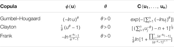
TABLE 1. List of common Archimedean copula function.

Joint Probability Analysis Based on Copulas

A d-dimensional joint distribution probability can be defined as follows (Song, 2012):

$F_{X_1{X}_2\dots X_d}\left(x_1,x_2,\dots ,x_d\right)=P\left(X_1\le x_1,X_2\le x_2,\dots ,X_d\le x_d\right)=\underset{-\infty }{\overset{x_1}{{\displaystyle \int }}}\underset{-\infty }{\overset{x_2}{{\displaystyle \int }}}\dots \underset{-\infty }{\overset{x_d}{{\displaystyle \int }}}{f}_{X_1{X}_2\dots X_d(w_1,w_2,\mathrm{..},w_d)}d{w}_{1}d{w}_2\mathrm{..}d{w}_d,(6)$

where $f_{X_1{X}_2\dots X_d(w_1,w_2,\mathrm{..},w_d)}$ is the density function of X₁, X₂, … , X_d. The marginal probability distributions of X₁, X₂, … , X_d are denoted by $F_{X_1\left({\text{x}}_1\right)}=P(X_1\le x_1),F_{X_2\left({\text{x}}_2\right)}=P(X_2\le x_2)$,…, $F_{X_{\text{d}}\left({\text{x}}_{\text{d}}\right)}=P(X_d\le x_d)$.

Similar to the classification of wet–dry season, it is a common practice to classify runoff as wet, median, and dry periods according to the result of the frequency analysis in China to facilitate the management of watershed management. The common classification criterion is the cumulative probability distribution method.

$\begin{array}{l}P\left(X<X_i\right)<P_d : dry year,\\ P_d<P\left(X<X_i\right)<P_w :median water year,and\\ P\left(X<X_i\right)>P_w : wet year.\end{array}(7)$

where $P_d$ and $P_w$ are the thresholds of classification. $P\left(X<X_i\right)$ is the cumulative probability distribution of runoff value X. Combined with the copula function, the dryness–wetness encounter probabilities of water replenishment resources are transformed into the multivariate joint probability.

For the bivariate joint probability, let $X_d$ and $X_w$, $Y_d$, and $Y_w$ be the thresholds of wet–dry classification of two runoff series, respectively. According to the probability inclusion–exclusion principle, the combination type can be calculated as follows:

Synchronization probability is given as follows:

$\mathrm{Dry}-\mathrm{dry}P\left(X<X_d,Y<Y_d\right)=c\left(X_d ,Y_w\right),$

$\mathrm{Median}-\mathrm{median}P\left(X_d<X<X_w,Y_d<Y<Y_w\right)=c\left(X_w ,Y_w\right)-c\left(X_d ,Y_w\right)-c\left(X_w ,Y_d\right)+c\left(X_d ,Y_d\right),$

$\mathrm{Wet}-\mathrm{wet}P\left(X>X_w,Y>Y_w\right)=1-P_w-P_w+c\left(X_w ,Y_w\right).$

Asynchronous probability is

$\mathrm{Dry}-\mathrm{median}P\left(X<X_d,Y_d<Y<Y_w\right)=c\left(X_d ,Y_w\right)-c\left(X_d ,Y_d\right),$

$\mathrm{Dry}-\mathrm{wet}P\left(X<X_d,Y>Y_w\right)=P_d-c\left(X_d ,Y_w\right),$

$\mathrm{Median}-\mathrm{dry}P\left(X_d<X<X_w,Y<Y_d\right)=c\left(X_w ,Y_d\right)-c\left(X_d ,Y_d\right),$

$\mathrm{Median}-\mathrm{wet}P\left(X_d<X<X_w,Y>Y_w\right)=P_w-P_d-c\left(X_w ,Y_w\right)+ c\left(X_d ,Y_w\right),$

$\mathrm{Wet}-\mathrm{dry}P\left(X>X_w,Y<Y_d\right)=P_d-c\left(X_w ,Y_d\right),and$

$\mathrm{Wet}-\mathrm{median}P\left(X>X_w,Y_d<Y<Y_w\right)=P_w-P_d-c\left(X_w ,Y_w\right)+c\left(X_w ,Y_d\right).$

For the trivariate joint probability, there are 3³ = 27 combination types based on the probability inclusion–exclusion principle. No more details are provided here, except the diagrammatic sketch (Figure 1B), due to limited space.

FIGURE 1

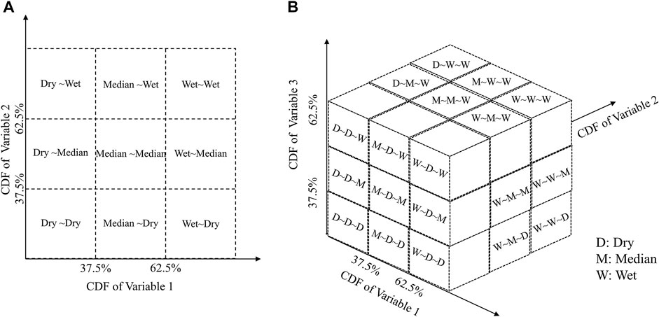
FIGURE 1. Sketch of the dryness–wetness encounter probabilities: (A) bivariate joint probability and (B) trivariate joint probability.

Conditional probability is also employed in the analysis of the dryness–wetness encounter probability. Conditional probability is defined as the likelihood of an event or outcome occurring, based on the occurrence of a previous event.

$\mathbf{P}\left(\mathbf{A}\text{|}\mathbf{B}\right)=\mathbf{P}\left(\mathbf{AB}\right)/\mathbf{P}\left(\mathbf{B}\right),(8)$

where $P\left(A\text{|}B\right)$ is the probability of event A occurring given that event B has already occurred. $P\left(AB\right)$ is the joint probability of events A and B. $P\left(B\right)$ is the probability of event B.

Study Area and Data

The BaiYangDian Lake (the BYD Lake) is located in the Haihe River Basin, which is the largest shallow lake/wetland in the North China plain. In the past 50 years, climate changes and human impacts have led to a sharp decrease in the amount of water entering the lake, and the water level in the lake has dropped significantly (Hu et al., 2012). According to the measured data of the Zaolinzhuang station at the outlet of the BYD Lake, the average water level was 7.67 m in 1950, and by 2018, it was only 6.88 m. The maximum water depth is 5∼6m, and the average water depth is only 1∼2 m. The decline of water level led to frequent drying up of the BYD Lake. In the 1970s, the lake dried up for 647 days in 1970–1973 and 1976. In the 1980s, the lake dried up for 6 years in a row from 1983 to 1988, for a total of 1845 days. In the 2000s, the lake dried up for a total of 1,488 days between 2000 and 2008. Low water-level events that occurred frequently and for a long time wreaked havoc on the lake’s ecological health (Xu et al., 2011; Yang et al., 2016). The ecological restoration of the BYD Lake is nearing completion, and water replenishment via water transfer projects is one of the most efficient ways to meet the ecological water demand while also addressing the local water shortage.

Three water sources of EWR are available. The upstream reservoirs (the Wangkuai Reservoir, the Xidayang Reservoir, and the Angezhuang Reservoir) are important water sources as local water resources. The total annual runoff of the three reservoirs is less than 0.1 billion m³. The targets are urban, agricultural, and ecological water consumption downstream of the BYD Basin. The locations of the three reservoirs and the BYD Lake are shown in Figures 2B. Except for the upstream reservoirs, two water transfer projects have been in operation for the EWR of the BYD Lake.

1) Danjiangkou Reservoir (DJK) in the Hanjiang River Basin. The SNWDP is a large-scale water diversion project led by the Chinese government, which transfers water from DJK to northern China. The project was completed and put into operation in December 2014, and the BYD Lake received its first ecological water replenishment via the SNWDP in 2018. The average annual inflow of the DJK reservoir is over 35 billion m³, and the average annual water diversion of the SNWDP is 8.54 billion m³. The main targets are 14 cities in northern China, including Beijing and Tianjin, that are suffering from water resources’ shortage. It is worth mentioning that the SNWDP targets have substantial water use competition. The amount of water that can be used for ecological water replenishment is only 0.1–0.3 billion m³.

2) The mainstream of the Yellow River. The Yellow River Diversion Project is also a comprehensive large-scale water transfer project, which transfers water from the lower Yellow River to the BYD Lake. The targets of the project are the BYD Lake and five cities along the way. The project was completed and put into operation in November 2017. The annual average runoff at the Huayuankou section of the Yellow River (HYK) is 34.9 billion m³. HYK is a large hydrological station nearest to the water intake position of the project. The annual average water diversion of the project is 0.62 billion m³ and the amount of water that can flow in the BYD Lake is about 0.1 billion m³.

FIGURE 2

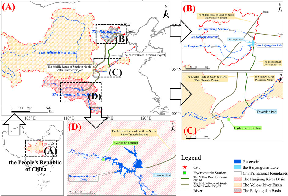
FIGURE 2. Location of the research area.

In general, the annual average runoff is large, but the amount for the water transfer project is small and the amount flowing into the BYD Lake is tiny. The transferable water quantity of the water sources is limited during a dry year, and it is difficult to guarantee the water demand of the BYD Lake using a single water source. Therefore, EWR of the BYD Lake from multiple water sources and the consequent analyses of dryness–wetness encounter probabilities among multiple water sources are necessary and meaningful.

The data used in this article include 1) the annual inflow of Danjiangkou Reservoir (DJK), 2) the annual runoff measuring at Huayuankou section of the Yellow River (HYK), and 3) the total annual inflow of the upstream three reservoirs, including the Wangkuai Reservoir, the Xidayang Reservoir, and the Angezhuang Reservoir (UR). The dataset with strict quality control covers 1961–2018 and is acquired from “Annual Hydrological Report P.R China” released by the Chinese government. It is worth noting that the EWR of the BYD Lake has only been operational since 2017. Long-term observation data after the EWR operation cannot be able to obtained. The non-stationarity of the dataset will be given full consideration in this study. What is more, the hydrometric stations observing this dataset are located upstream of the diversion ports (as shown in Figure 2), effectively avoiding the impact of water diversion projects’ construction on data observation. Given the reasons, it is believed that the long-term datasets were of a good quality, which could fit the requirement of the dryness–wetness encounter probability analysis in this study.

Results and Discussion

Trend and Change Points Analysis

Hydrological series are generally composed of deterministic aperiodic components, deterministic periodic components, and stochastic components (Xinan and Ping, 2012). The deterministic aperiodic components include transient components such as trend and change point, which are often superimposed on other components. When the hydrological time series has a significant trend and change point, it is no longer consistent. The traditional frequency analysis is based on the consistency of hydrological series, so the trend and mutation point should be tested before fitting the marginal distribution.

The trend test results are shown in Table 2. The annual runoff series of DJK, HYK, and UR have decreasing trends. The annual changing rates in HYK and UR are −5.4042 and −0.1877 billion m³/10a, respectively. HYK’s annual runoff was approximately 34.9 billion m³ in 1961–2018 and 28 billion m³ in 2009–2018, while that of UR was 0.959 and 0.590 billion m³, respectively. The result indicates that the decreasing trends in HYK and UR are significant (p value < 0.01). For DJK, the significance of the decreasing trend does not reach up to 0.05 level.

TABLE 2

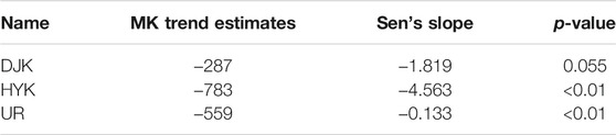
TABLE 2. Results of MK and Sen’s slope trend tests from 1961 to 2018.

Pettitt, SNHT, and Mann–Kendall tests were employed to analyze the change point of the annual runoff series in DJK, HYK, and UR (Table 3). The change point is 1990 in DJK. Some studies (Dongfei et al., 2016) suggested that the runoff decreased sharply because of the great climate change around 1990, such as the decrease of precipitation and the increase of temperature. The change points are 1985 and 1990 in HYK. Some studies (Jun et al., 2014) found that the atmospheric circulation in this area was abnormal from 1985 to 1990. The Mongolian low pressure significantly weakened and the summer monsoon was weak, resulting in a decrease in the precipitation and then in the runoff. The change point is 1996 in UR. Some studies (Ling-ling and Si-rui, 2016) believed that the abnormal decrease of runoff was caused by the change of the runoff generation mechanism. Linear regression curve and mean values before/after change points are shown in Figure 3.

TABLE 3

TABLE 3. Results of Pettitt, SNHT, and Lanzante tests for change point from 1961 to 2018.

FIGURE 3

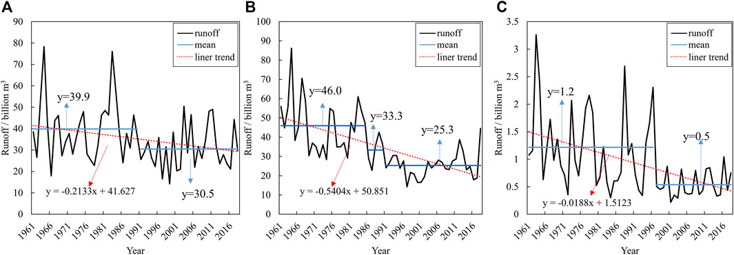
FIGURE 3. Linear regression curve and mean values before and after change points from 1961 to 2018: (A) DJK, (B) HYK, and (C) UR.

From the results of trend and change point analysis, it is clear that the runoff in the regions of the three water sources showed significant non-stationarity in the past decades, which is in accordance with the previous studies. The annual runoff (2009–2018) of three hydrological stations in the middle reaches of the Yellow River decreased by 14.33%, 32.16%, 40.79%, and 44.32% compared with the maximum annual runoff (1959–1968) at each station (Wang and Sun, 2021). The results of the other two water sources with decreased trends are also supported by previous studies (Chen et al., 2007; Wang et al., 2021). In short, before conducting a hydrological frequency analysis, the non-stationarity of the runoff series must be considered in the planning and construction of water infrastructures including interbasin water transfer projects, reservoirs, and groundwater projects (Dong and Zhang, 2014; Isensee et al., 2021).

Marginal Distribution Fitting Based on the GAMLSS Model

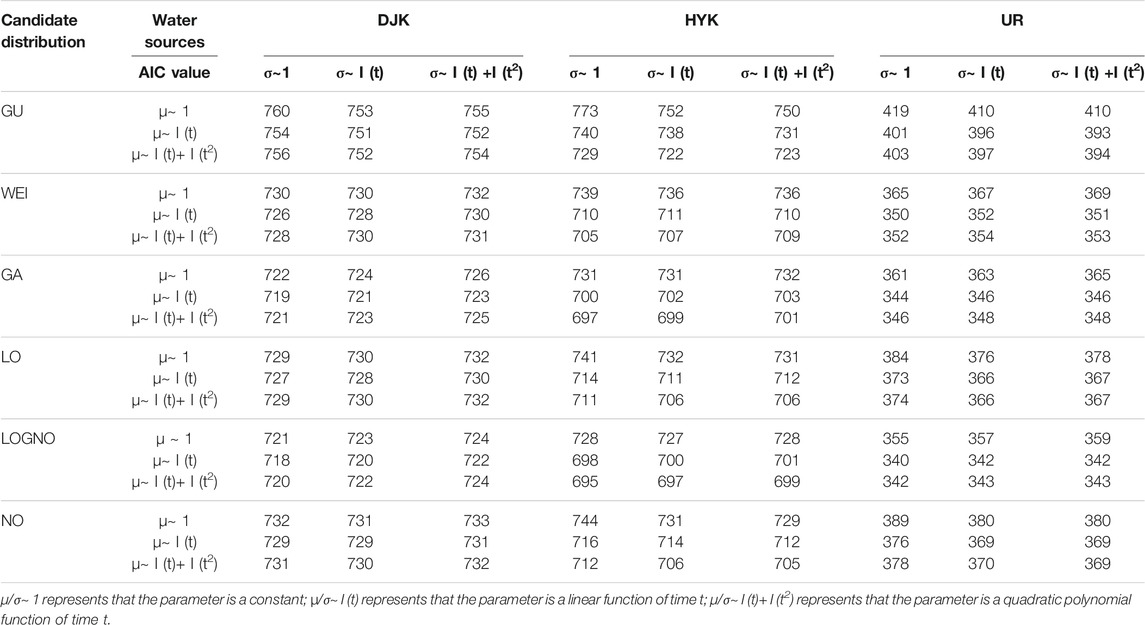
Annual runoff series were non-stationary, according to the above results, due to change points and trends. Based on the result of the consistency test in Section 4.1, the GAMLSS model was employed to fit the marginal distributions of annual runoff in DJK, HY, and UR. Gumbel (GU), Weibull (WEI), gamma (GA), logistic (LO), log normal (LOGNO), and normal distribution (NO) were the candidate distributions. There were two types of fitting: (A) stationary marginal distributions and (B) time-varying marginal distributions with time as the explanatory variable. The position parameter μ and scale parameter σ were regarded as time-varying parameters to avoid overly complex regression equation, while shape parameter ν was assumed as a constant; that is, 1) both μ and σ are constants; 2) μ is a polynomial function of time t, while σ is a constant; 3) σ is a polynomial function of time t, while μ is a constant; and 4) both μ and σ are polynomial functions of time t. Only the linear and quadratic polynomial functions are included. The Akaike information criterion (AIC) was used to evaluate the goodness of fit of the distribution models and functions. The worm plot was used for visualizing the fitting performance of candidate models.

The complete results of marginal distribution fitting are given in Appendix Table A1. Table 4 shows the distribution name, distribution parameters, and AIC of the selected optimal marginal distribution. The marginal distribution fitting results of stationary type, namely, both μ and σ are constants, are also listed in the table for comparison. As shown in Table 4, for the annual runoff series with significant change points (like HJK and UR), non-stationary and stationary models had distinctly different AIC values. However, for the modeling of annual runoff series with the narrow changing range before and after their change points, non-stationary and stationary models had similar AIC values, which indicates that time-varying marginal distributions are suitable to capture the non-stationary characteristics. According to the AIC values, non-stationary models perform better than stationary models. The position parameter of the log-normal distribution for describing runoff series at DJK, HYK, and UR relates to the time (explanatory variable) negatively, whereas the scale parameter is constant. Therefore, the log-normal distribution with time-varying parameters is the selected optimal marginal distribution for the annual runoff series of DJK, HYK, and UR.

TABLE 4

TABLE 4. Results of marginal distributions fitting using the GAMLSS model.

Analysis of residuals is necessary to evaluate the performance of the selected models. Figure 4 demonstrates the worm plots of the residuals by GAMLSS for the selected optimal marginal distributions in Table 4. It can be observed from the figure that the sample points of the annual runoff series follow the red solid curves fluctuating between two dashed curves, implying that the selected models have a quite good fitting quality at the 95% confidence level.

FIGURE 4

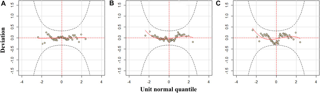
FIGURE 4. Worm plot of the residuals by GAMLSS for annual runoff series at (A) DJK, (B) HYK, and (C) UR.

Figure 5 shows the comparison of the cumulative probability distribution of the selected models. CDF_s and CDF_n mean the cumulative probability distribution function of the stationary model and the non-stationary model, respectively. The bars are the difference between the two (CDF_s—CDF_n). The green vertical lines are change points of the annual runoff series. The CDF of the selected non-stationary model is different from that of the stationary model. Before the change point, the CDF is greater than that of the stationary model (CDF_s > CDF_n), while it is reversed after the change point (CDF_s < CDF_n). Considering the decreasing trend of annual runoff in DJK, HYK, and UR, it is easy to be understood.

FIGURE 5

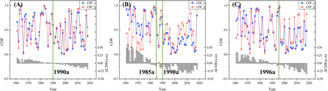
FIGURE 5. Comparison of the cumulative probability distribution for annual runoff series at (A) DJK, (B) HYK, and (C) UR.

In China, it is a common practice to classify runoff as wet, median, or dry periods based on the results of frequency analysis to facilitate water resource management. Typically, $P_d$ and $P_w$ are 37.5% and 62.5%, respectively. According to the above, the choice of the stationary or non-stationary model will change the CDF of the annual runoff, which in turn changes classification results (Figure 6). The transfer matrix from the stationary to non-stationary model in DJK indicated shows that 8 out of 58 years in the classification result changed. For HYK and UR, the amount of change years is 29 and 19, respectively. This also indicates that the traditional runoff classification without considering non-stationary is not accurate enough. Based on this fact, we further calculated the dryness–wetness encounter probability of annual runoff in DJK, HYK, and UR, using the non-stationary model.

FIGURE 6

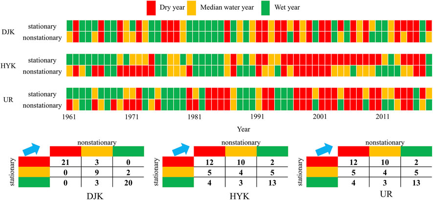
FIGURE 6. Classification results and transfer matrices of runoff series based on the stationary model against the non-stationary model in DJK, HYK, and UR (red: dry year; yellow; median water year; and green: wet year).

The Dryness–Wetness Encounter Probability Based on the Copula Function

Clayton copula, Gumbel–Hougaard copula, and Frank copula were selected as candidate distributions to construct bivariate and trivariate joint distribution functions. The maximum likelihood method is used to estimate the parameters of the copula function. The Akaike information criterion (AIC) and the Cramér-von Mises test (Genest et al., 2009) were used to evaluate the goodness of fit of the copula function. Table 5 summarizes the results of parameter estimation and goodness-of-fit testing for three candidate copulas. Bold text means the selected copulas in this study. Since the correlation between DJK and UR is negative, the Gumbel–Hougaard copula that allows only for positive dependence variables was excluded from the candidate distributions. As shown in Table 5, the selected optimal copulas for DJK-HYK, DJK-UR, and HYK-UR were Gumbel copula, Frank copula, and Clayton copula respectively. And Clayton copula was the optimal copula for DJK-HYK-UR.

TABLE 5

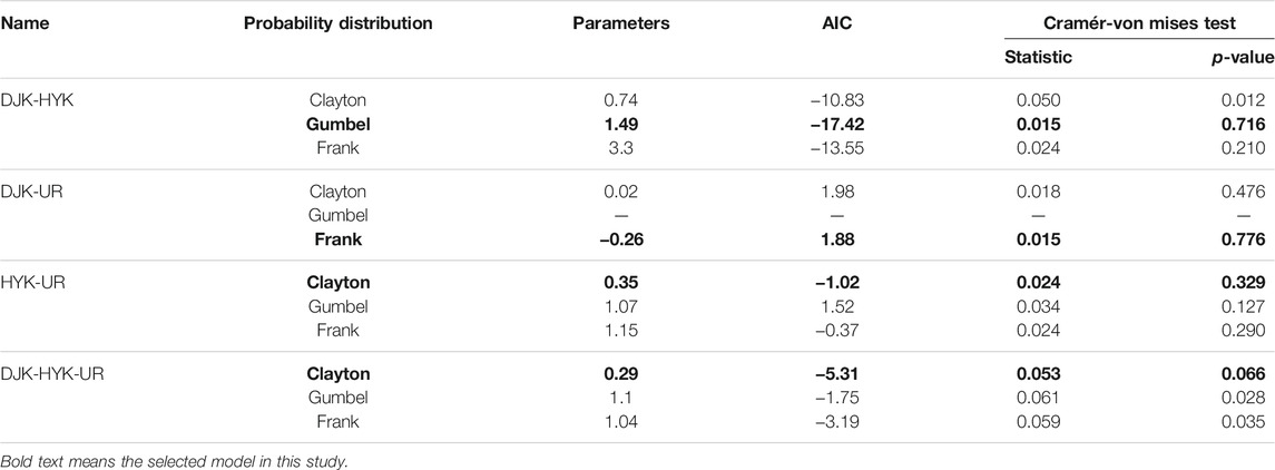
TABLE 5. Parameter estimation and goodness-of-fit testing of copulas.

According to the selected optimal copula and the parameter estimated by the maximum likelihood method, the bivariate and trivariate joint distributions are the probability of the annual runoff series. As mentioned earlier, $P_d$ and $P_w$ are 37.5% and 62.5%, respectively, in the runoff classification analysis. We classified runoff as wet, median, and dry periods according to Eq. 7, and then the encounter probability of bivariate combination types was calculated using the probability inclusion–exclusion principle (Table 6).

TABLE 6

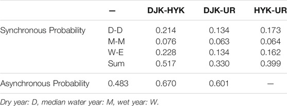
TABLE 6. Encounter probability of bivariate combination types.

For the encounter probability of bivariate combination types, the asynchronous probabilities of DJK-UR and HYK-UR are over 0.6. It seems reasonable as HYK is to the south of UR and DJK is more south geographically (Figure 2). Different geographical locations lead to differences in factors such as climate and vegetation, and further lead to a higher asynchronous probability of runoff series. The result also indicates that the interbasin water transfer project is a reasonable way for EWR of the BYD Lake.

For the encounter probability of trivariate combination types, the result of 27 types is presented in Table 7. The synchronous probability of runoff series of three water sources, namely, the synchronous case ($P_S=P(D\&D\&D)+P(M\&M\&M)+P(W\&W\&W)$) is only 0.180. The asynchronous probability is higher than the bivariate combination types. But it is also noted that the asynchronous probability of DJK and HYK is 0.602, which indicates that there is no substitution between the two water sources. DJK and HYK are both important and necessary sources of EWP for the BYD Lake. A single water source is difficult to guarantee the ecological water demand of the BYD Lake. We suggest that the designed annual replenishment water amount of the BYD Lake should be adjusted to adapt to the wetness–dryness situation of DJK and HYK.

TABLE 7

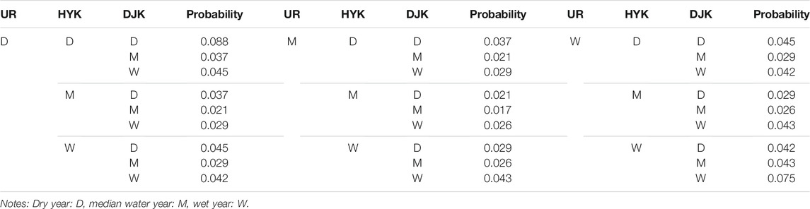
TABLE 7. Encounter probability of trivariate combination types.

Because the BYD Lake and the three upstream reservoirs (UR) are in the same watershed, the dryness–wetness situation of UR represents, to some extent, the ecological water replenishment demand of the BYD Lake. Table 8 shows the result of conditional encounter probability. During a dry year of UR, the conditional probability that neither DJK nor HYK is in a dry year is 0.465. In this scenario, water from other watersheds partially meets BYR’s water demand. But the conditional probability that both DJK and HYK are in a dry year is 0.234. Thus, to solve the problem of not having enough water, some additional water resources and a reasonable EWR plan are required.

TABLE 8

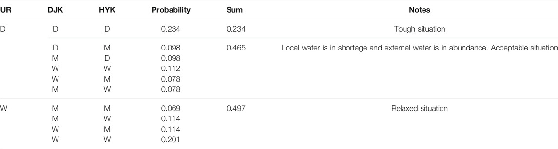
TABLE 8. Conditional encounter probability.

The grim situation could be avoided by reservoir regulation, activating emergency water source and diversifying water sources (such as recycled water).

It is worth noting that 1) the probability that the water supply situation is tough is only calculated by the runoff series classification of each water source, not a direct comparison of water quantity. Perhaps when DJK or HYK is in a dry year, the amount of water that can be transferred into the BYD Lake is enough to meet the ecological water replenishment demand. In this case, the available amount of ecological water replenishment is only limited by the design amount of the water diversion projects. In other words, we only examined the water supply situation from the perspective of the water source, without considering the quantity of water diversion and water supply available from the water transfer projects. 2) DJK and UR are the reservoirs with regulating water storage capacity. The data used in this article are the inflow runoff series of reservoirs. The available water quantity of the water transfer projects is ultimately determined by the water level in the downstream area of the reservoirs.

Despite the limitations mentioned earlier, the results of encounter probability analysis could assist EWR project decision-makers in fully understanding potential challenges and devising appropriate countermeasures, and thus ensure the effectiveness of ecological replenishment projects. We believe that this article provides a research approach for EWR via interbasin water transfer projects that can capture the non-stationarity of runoff series and speculate on possible scenarios during the project operation phase. Current studies about EWR focus on targets’ water demand and give simple constraints for water diversion and supplementation amount in their water replenishment optimization model (Huang et al., 2021). If more attention was paid to analyzing the non-stationarity and the dryness–wetness encounter probability, the optimization model would be more reasonable. Indeed, a large number of interbasin water transfer projects have been or are being built for the purpose of overcoming water scarcity and alleviating environmental problems (Guo et al., 2012; Akron et al., 2017; Roozbahani et al., 2020; Lei et al., 2021; Sun et al., 2021), which provides opportunities for the approach’s application.

Conclusion

This article aimed to investigate the dryness–wetness encounter probability of runoff series between the lake replenishment water sources. The dryness–wetness bivariate and trivariate encounter probability analyses under non-stationary conditions is investigated in this study. Non-stationary frequency analysis is modeled with time as the explanatory variable using GAMLSS. The joint probability of runoff series using copula is calculated to assess the dryness–wetness encounter probability. The main results of this study are as follows:

Significant non-stationarity has been detected for DJK, HYK, and UR. Using MK and Sen’s slope trend tests, there was a gradual fall in the runoff series of DJK and sharp drops in HYR and UR. Using Pettitt, SNHT, and Mann–Kendall tests, 1990, 1985, and 1990, and 1996 are considered as the change points of runoff in DJK, HYR, and UR, respectively.

The non-stationary model with time as the explanatory variable is more suitable for the runoff series of DJK, HYK, and UR. Under the non-stationary framework, the wet–dry classification of runoff series is completely changed. The transfer matrix from the stationary to non-stationary model in DJK indicated shows that eight out of 58 years in the classification result changed. For HYK and UR, the amount of change years is 29 and 19, respectively.

For the encounter probability of bivariate combination types, the asynchronous probabilities of DJK-UR and HYK-UR are over 0.6, which indicates that the interbasin water transfer project is a reasonable and scientific way for the BYD Lake ecological water replenishment.

For the encounter probability of trivariate combination types, the asynchronous probability of runoff series of three water sources (P_A) is 0.82, and the asynchronous probability of DJK and HYK is 0.602, which indicates that there is no substitution between DJK and HYK. A single water source is difficult to guarantee the ecological water demand of the BYD Lake.

During a dry year of UR, the conditional probability that both DJK and HYK are in a dry year is 0.234. Thus, some additional water resources and a reasonable EWR plan are required to solve the case when no water is available.

Data Availability Statement

The original contributions presented in the study are included in the article/Supplementary Material, further inquiries can be directed to the corresponding author.

Author Contributions

Contributions to conception and design: YX, FL, and BR; acquisition of data, methodology, and analysis: YX, YZ, YD, and KW; writing—original draft: YX; writing—review and editing: YX, FL, YZ, BR, YD, and KW.

Funding

This study was financially supported by the National Key Research and Development Plan of China (No. 2018YFC0406506) and the National Natural Science Foundation of China (No. 51679252).

Conflict of Interest

The authors declare that the research was conducted in the absence of any commercial or financial relationships that could be construed as a potential conflict of interest.

Publisher’s Note

All claims expressed in this article are solely those of the authors and do not necessarily represent those of their affiliated organizations, or those of the publisher, the editors, and the reviewers. Any product that may be evaluated in this article, or claim that may be made by its manufacturer, is not guaranteed or endorsed by the publisher.

References

Acreman, M. C., Fisher, J., Stratford, C. J., Mould, D. J., and Mountford, J. O. (2007). Hydrological Science and Wetland Restoration: Some Case Studies from Europe. Hydrol. Earth Syst. Sci. 11, 158–169. doi:10.5194/hess-11-158-2007

CrossRef Full Text | Google Scholar

Ahn, K.-H., and Palmer, R. N. (2016). Use of a Nonstationary Copula to Predict Future Bivariate Low Flow Frequency in the Connecticut River Basin. Hydrol. Process. 30, 3518–3532. doi:10.1002/hyp.10876

CrossRef Full Text | Google Scholar

Akron, A., Ghermandi, A., Dayan, T., and Hershkovitz, Y. (2017). Interbasin Water Transfer for the Rehabilitation of a Transboundary Mediterranean Stream: An Economic Analysis. J. Environ. Manage. 202, 276–286. doi:10.1016/j.jenvman.2017.07.043

CrossRef Full Text | Google Scholar

Alexandersson, H. (1986). A Homogeneity Test Applied to Precipitation Data. J. Climatol. 6, 661–675. doi:10.1002/joc.3370060607

CrossRef Full Text | Google Scholar

Ariff, N. M., Jemain, A. A., Ibrahim, K., and Wan Zin, W. Z. (2012). IDF Relationships Using Bivariate Copula for Storm Events in Peninsular Malaysia. J. Hydrol. 470-471, 158–171. doi:10.1016/j.jhydrol.2012.08.045

CrossRef Full Text | Google Scholar

Chen, H., Guo, S., Xu, C.-y., and Singh, V. P. (2007). Historical Temporal Trends of Hydro-Climatic Variables and Runoff Response to Climate Variability and Their Relevance in Water Resource Management in the Hanjiang basin. J. Hydrol. 344, 171–184. doi:10.1016/j.jhydrol.2007.06.034

CrossRef Full Text | Google Scholar

Chen, Y., Zong, Y., Li, B., Li, S., and Aitchison, J. C. (2013). Shrinking Lakes in Tibet Linked to the Weakening Asian Monsoon in the Past 8.2 Ka. Quat. Res. 80, 189–198. doi:10.1016/j.yqres.2013.06.008

CrossRef Full Text | Google Scholar

Cong, Z., Yang, D., Gao, B., Yang, H., and Hu, H. (2009). Hydrological Trend Analysis in the Yellow River basin Using a Distributed Hydrological Model. Water Resour. Res. 45, W00A13. doi:10.1029/2008WR006852

CrossRef Full Text | Google Scholar

Ding, Y., Liu, H., Yang, W., Xing, L., Tu, G., Ru, Z., et al. (2019). The Assessment of Ecological Water Replenishment Scheme Based on the Two-Dimensional Lattice-Boltzmann Water Age Theory. J. Hydro-Environ. Res. 25, 25–34. doi:10.1016/j.jher.2019.07.001

CrossRef Full Text | Google Scholar

Dong, Q., and Zhang, Y. (2014). Advances in Research of Hydrological Serial Variation under Non-stationary Conditions and Their Impacts on Flood Control of Reservoirs. Adv. Sci. Technol. Water Resour. 34, 71–75. doi:10.1007/s11032-014-0087-2

CrossRef Full Text | Google Scholar

Dongfei, Y., Jiancang, X., Rengui, J., Hao, W., and Yang, L. (2016). Trends and Characteristics of Runoff for Upper Hanjiang River. J. Water Resour. Water Eng. 27, 13–19. doi:10.11705/j.issn.1672-643X.2016.06.03

CrossRef Full Text | Google Scholar

Du, T., Xiong, L., Xu, C.-Y., Gippel, C. J., Guo, S., and Liu, P. (2015). Return Period and Risk Analysis of Nonstationary Low-Flow Series under Climate Change. J. Hydrol. 527, 234–250. doi:10.1016/j.jhydrol.2015.04.041

CrossRef Full Text | Google Scholar

Feng, P., Niu, J. Y., Zhang, Y., and Hou, H. Y. (2010). Analysis of Wetness-Dryness Encountering Probability Among Water Source Rivers and the Yellow River in the Western Route of South-To-North Water Transfer Project. J. Hydraul. Eng. 41, 900–907. doi:10.3724/SP.J.1084.2010.00199

CrossRef Full Text | Google Scholar

Feng, Y., Shi, P., Qu, S., Mou, S., Chen, C., and Dong, F. (2020). Nonstationary Flood Coincidence Risk Analysis Using Time-Varying Copula Functions. Sci. Rep. 10, 3395. doi:10.1038/s41598-020-60264-3

PubMed Abstract | CrossRef Full Text | Google Scholar

Genest, C., and Favre, A.-C. (2007). Everything You Always Wanted to Know about Copula Modeling but Were Afraid to Ask. J. Hydrol. Eng. 12, 347–368. doi:10.1061/(asce)1084-0699(2007)12:4(347)

CrossRef Full Text | Google Scholar

Genest, C., Rémillard, B., and Beaudoin, D. (2009). Goodness-of-fit Tests for Copulas: A Review and a Power Study. Insurance: Math. Econ. 44, 199–213. doi:10.1016/j.insmatheco.2007.10.005

CrossRef Full Text | Google Scholar

Gocic, M., and Trajkovic, S. (2013). Analysis of Changes in Meteorological Variables Using Mann-Kendall and Sen's Slope Estimator Statistical Tests in Serbia. Glob. Planet. Change 100, 172–182. doi:10.1016/j.gloplacha.2012.10.014

CrossRef Full Text | Google Scholar

Grimaldi, S., and Serinaldi, F. (2006). Asymmetric Copula in Multivariate Flood Frequency Analysis. Adv. Water Resour. 29, 1155–1167. doi:10.1016/j.advwatres.2005.09.005

CrossRef Full Text | Google Scholar

Guo, X., Hu, T., Zhang, T., and Lv, Y. (2012). Bilevel Model for Multi-Reservoir Operating Policy in Inter-basin Water Transfer-Supply Project. J. Hydrol. 424-425, 252–263. doi:10.1016/j.jhydrol.2012.01.006

CrossRef Full Text | Google Scholar

Hu, S., Liu, C., Zheng, H., Wang, Z., and Yu, J. (2012). Assessing the Impacts of Climate Variability and Human Activities on Streamflow in the Water Source Area of Baiyangdian Lake. J. Geogr. Sci. 22, 895–905. doi:10.1007/s11442-012-0971-9

CrossRef Full Text | Google Scholar

Huang, J., Zhao, L., and Sun, S. (2021). Optimization Model of the Ecological Water Replenishment Scheme for Boluo Lake National Nature Reserve Based on Interval Two-Stage Stochastic Programming. Water 13, 1007. doi:10.3390/w13081007

CrossRef Full Text | Google Scholar

Isensee, L. J., Pinheiro, A., and Detzel, D. H. M. (2021). Dam Hydrological Risk and the Design Flood under Non-stationary Conditions. Water Resour. Manage. 35, 1499–1512. doi:10.1007/s11269-021-02798-3

CrossRef Full Text | Google Scholar

Jia, Y., Ding, X., Wang, H., Zhou, Z., Qiu, Y., and Niu, C. (2012). Attribution of Water Resources Evolution in the Highly Water-Stressed Hai River Basin of China. Water Resour. Res. 48, W02513. doi:10.1029/2010WR009275

CrossRef Full Text | Google Scholar

Jiang, C., Xiong, L., Xu, C.-Y., and Guo, S. (2015). Bivariate Frequency Analysis of Nonstationary Low-Flow Series Based on the Time-Varying Copula. Hydrol. Process. 29, 1521–1534. doi:10.1002/hyp.10288

CrossRef Full Text | Google Scholar

Jones, B. A., and Fleck, J. (2020). Shrinking Lakes, Air Pollution, and Human Health: Evidence from California’s Salton Sea. Sci. Total Environ. 712, 136490. doi:10.1016/j.scitotenv.2019.136490

PubMed Abstract | CrossRef Full Text | Google Scholar

Jun, C., Yu, Z., and Xuan, Z. (2014). Relationship between Runoff of Huayuankou Station on Yellow River and Atmospheric Circulation Anomalies. Yellow River 36, 11–13.

Google Scholar

Kummu, M., Guillaume, J. H. A., de Moel, H., Eisner, S., Flörke, M., Porkka, M., et al. (2016). The World's Road to Water Scarcity: Shortage and Stress in the 20th century and Pathways towards Sustainability. Sci. Rep. 6, 38495. doi:10.1038/srep38495

PubMed Abstract | CrossRef Full Text | Google Scholar

Kwon, H.-H., and Lall, U. (2016). A Copula-Based Nonstationary Frequency Analysis for the 2012-2015 Drought in California. Water Resour. Res. 52, 5662–5675. doi:10.1002/2016wr018959

CrossRef Full Text | Google Scholar

Lei, G. J., Wang, W. C., Liang, Y., Yin, J. X., and Wang, H. (2021). Failure Risk Assessment of Discharge System of the Hanjiang-To-Weihe River Water Transfer Project. Nat. Hazards 108, 3159–3180. doi:10.1007/s11069-021-04818-2

CrossRef Full Text | Google Scholar

Li, J., Lei, Y., Tan, S., Bell, C. D., Engel, B. A., and Wang, Y. (2018). Nonstationary Flood Frequency Analysis for Annual Flood Peak and Volume Series in Both Univariate and Bivariate Domain. Water Resour. Manage. 32, 4239–4252. doi:10.1007/s11269-018-2041-2

CrossRef Full Text | Google Scholar

Libiseller, C., and Grimvall, A. (2010). Performance of Partial Mann–Kendall Tests for Trend Detection in the Presence of Covariates. Environmetrics 13, 71–84. doi:10.1002/env.507

CrossRef Full Text | Google Scholar

Ling-ling, C., and Si-rui, C. (2016). Analysis of the Reliability and Consistency of Rainfall Run-Off in Xidayang Reservoir. Water Sci. Eng. Technol. 4, 1–4,5. doi:10.19733/j.cnki.1672-9900.2016.04.001

CrossRef Full Text | Google Scholar

Liu, H., Chen, Y., Ye, Z., Li, Y., and Zhang, Q. (2019). Recent Lake Area Changes in Central Asia. Sci. Rep. 9, 16277. doi:10.1038/s41598-019-52396-y

PubMed Abstract | CrossRef Full Text | Google Scholar

Liu, Z., Tan, S., Luo, Y., and Guan, S. (2015). Study of the Wetness-Dryness Encountering of Inflow of the Three Biggest Reservoirs in the Dongjiang River basin Based on Copula Functions. J. Lake Sci. 27, 361–370. doi:10.18307/2015.0222

CrossRef Full Text | Google Scholar

Lu, F., Wang, H., Yan, D., Zhang, D., and Xiao, W. (2013). Application of Profile Likelihood Function to the Uncertainty Analysis of Hydrometeorological Extreme Inference. Sci. China Technol. Sci. 56, 3151–3160. doi:10.1007/s11431-013-5421-0

CrossRef Full Text | Google Scholar

Mccuen, R. H. (1994). Time Series Modelling of Water Resources and Environmental Systems. J. Hydrol. 167, 399–400.

Google Scholar

Mei, X., Dai, Z., Du, J., and Chen, J. (2015). Linkage between Three Gorges Dam Impacts and the Dramatic Recessions in China's Largest Freshwater lake, Poyang Lake. Sci. Rep. 5, 18197. doi:10.1038/srep18197

PubMed Abstract | CrossRef Full Text | Google Scholar

Onuoha, F. C. (2008). Environmental Degradation, Livelihood and Conflicts: A focus on the Implications of the Diminishing Water Resources of Lake Chad for North-Eastern Nigeria. Afr. j. confl. resolut. 8, 35–61. doi:10.4314/ajcr.v8i2.39425

CrossRef Full Text | Google Scholar

Pettitt, A. N. (1979). A Non-Parametric Approach to the Change-Point Problem. Appl. Stat. 28, 126–135. doi:10.2307/2346729

CrossRef Full Text | Google Scholar

Ping, X., Guangcai, C., and Hongfu, L. (2009). Surface Water Resources Evaluation Methods on Changing Environment. Beijing,China: Science Press.

Google Scholar

Rashid, M. M., and Beecham, S. (2019). Simulation of Streamflow with Statistically Downscaled Daily Rainfall Using a Hybrid of Wavelet and GAMLSS Models. Hydrological Sci. J. 64, 1327–1339. doi:10.1080/02626667.2019.1630742

CrossRef Full Text | Google Scholar

Rigby, R. A., and Stasinopoulos, D. M. (2005). Generalized Additive Models for Location, Scale and Shape (With Discussion). J. R. Stat. Soc C 54, 507–554. doi:10.1111/j.1467-9876.2005.00510.x

CrossRef Full Text | Google Scholar

Roozbahani, A., Ghased, H., and Hashemy Shahedany, M. (2020). Inter-basin Water Transfer Planning with Grey COPRAS and Fuzzy COPRAS Techniques: A Case Study in Iranian Central Plateau. Sci. Total Environ. 726, 138499. doi:10.1016/j.scitotenv.2020.138499

PubMed Abstract | CrossRef Full Text | Google Scholar

Shiau, J. T., and Modarres, R. (2009). Copula-based Drought Severity-Duration-Frequency Analysis in Iran. Met. Apps 16, 481–489. doi:10.1002/met.145

CrossRef Full Text | Google Scholar

Sklar, M. (1959). Fonctions de repartition a n dimensions et leurs marges. Publ. Inst. Stat. Univ. Paris 8, 229–231.

Google Scholar

Song, S. (2012). Copulas Function and its Application in Hydrology. Beijing,China: Science Press.

Google Scholar

Stasinopoulos, D. M., and Rigby, R. A. (2007). Generalized Additive Models for Location Scale and Shape (GAMLSS) in R. J. Stat. Softw. 23, 1–46. doi:10.18637/jss.v023.i07

CrossRef Full Text | Google Scholar

Stone, R. (2021). After Revival, Iran's Great Salt lake Faces Peril. Science 372, 444–445. doi:10.1126/science.372.6541.444

PubMed Abstract | CrossRef Full Text | Google Scholar

Strupczewski, W. G., and Kaczmarek, Z. (2001). Non-stationary Approach to At-Site Flood Frequency Modelling II. Weighted Least Squares Estimation. J. Hydrol. 248, 143–151. doi:10.1016/s0022-1694(01)00398-5

CrossRef Full Text | Google Scholar

Strupczewski, W. G., Singh, V. P., and Mitosek, H. T. (2001). Non-stationary Approach to At-Site Flood Frequency Modelling. III. Flood Analysis of Polish Rivers. J. Hydrol. 248, 152–167. doi:10.1016/s0022-1694(01)00399-7

CrossRef Full Text | Google Scholar

Su, C., and Chen, X. (2019). Assessing the Effects of Reservoirs on Extreme Flows Using Nonstationary Flood Frequency Models with the Modified Reservoir index as a Covariate. Adv. Water Resour. 124, 29–40. doi:10.1016/j.advwatres.2018.12.004

CrossRef Full Text | Google Scholar

Sun, P., Wen, Q., Zhang, Q., Singh, V. P., Sun, Y., Li, J., et al. (2018). Nonstationarity-based Evaluation of Flood Frequency and Flood Risk in the Huai River basin, China. J. Hydrol. 567, 393–404. doi:10.2307/2346729

CrossRef Full Text | Google Scholar

Sun, S., Zhou, X., Liu, H., Jiang, Y., Zhou, H., Zhang, C., et al. (2021). Unraveling the Effect of Inter-basin Water Transfer on Reducing Water Scarcity and its Inequality in China. Water Res. 194, 116931. doi:10.1016/j.watres.2021.116931

PubMed Abstract | CrossRef Full Text | Google Scholar

Ting, Z., Yixuan, W., Bing, W., Senming, T., and Ping, F. (2018). Nonstationary Flood Frequency Analysis Using Univariate and Bivariate Time-Varying Models Based on GAMLSS. Water 10, 819. doi:10.3390/w10070819

CrossRef Full Text | Google Scholar

Ussenaliyeva, A., and Aizhan, U. (2020). Save Kazakhstan's Shrinking Lake Balkhash. Science 370, 1–303. doi:10.1126/science.abe7828

PubMed Abstract | CrossRef Full Text | Google Scholar

Villarini, G., Serinaldi, F., Smith, J. A., and Krajewski, W. F. (2009a). On the Stationarity of Annual Flood Peaks in the continental United States during the 20th century. Water Resour. Res. 45, 2263–2289. doi:10.1029/2008wr007645

CrossRef Full Text | Google Scholar

Villarini, G., Smith, J. A., Serinaldi, F., Bales, J., Bates, P. D., and Krajewski, W. F. (2009b). Flood Frequency Analysis for Nonstationary Annual Peak Records in an Urban Drainage basin. Adv. Water Resour. 32, 1255–1266. doi:10.1016/j.advwatres.2009.05.003

CrossRef Full Text | Google Scholar

Villarini, G., Smith, J. A., Serinaldi, F., Ntelekos, A. A., and Schwarz, U. (2012). Analyses of Extreme Flooding in Austria over the Period 1951-2006. Int. J. Climatol. 32, 1178–1192. doi:10.1002/joc.2331

CrossRef Full Text | Google Scholar

Vinnarasi, R., and Dhanya, C. T. (2019). Bringing Realism into a Dynamic Copula-Based Non-stationary Intensity-Duration Model. Adv. Water Resour. 130, 325–338. doi:10.1016/j.advwatres.2019.06.009

CrossRef Full Text | Google Scholar

Wang, H., Lv, X., and Zhang, M. (2021). Sensitivity and Attribution Analysis Based on the Budyko Hypothesis for Streamflow Change in the Baiyangdian Catchment, China. Ecol. Indic. 121, 107221. doi:10.1016/j.ecolind.2020.107221

CrossRef Full Text | Google Scholar

Wang, H., and Sun, F. (2021). Variability of Annual Sediment Load and Runoff in the Yellow River for the Last 100 Years (1919-2018). Sci. Total Environ. 758, 143715. doi:10.1016/j.scitotenv.2020.143715

PubMed Abstract | CrossRef Full Text | Google Scholar

Wang, L. D., Chun-San, Q. I., Cao, S. L., Xue, S. W., and Zhang, T. (2017). Analysis of Wetness-Dryness Compensation of the Yellow River,the Southeast and Northwest of Shandong Province. Water Resour. Power 35, 33–36. (in Chinese).

Google Scholar

Wang, Z., Wu, J., Madden, M., and Mao, D. (2012). China's Wetlands: Conservation Plans and Policy Impacts. Ambio 41, 782–786. doi:10.1007/s13280-012-0280-7

PubMed Abstract | CrossRef Full Text | Google Scholar

weigang, X., Yilei, Y., Muyuan, M., Yilei, Y., Muyuan, M., Jia, G., et al. (2018). Effects of Water Replenishment from Yellow River on Water Quality of Hengshui Lake 1 Wetland. Jmba 4, 11–13. doi:10.15436/2381-0750.18.1725

CrossRef Full Text | Google Scholar

Wen, T., Jiang, C., and Xu, X. (2019). Nonstationary Analysis for Bivariate Distribution of Flood Variables in the Ganjiang River Using Time-Varying Copula. Water 11, 746. doi:10.3390/w11040746

CrossRef Full Text | Google Scholar

Wu, P.-Y., You, G. J.-Y., and Chan, M.-H. (2020). Drought Analysis Framework Based on Copula and Poisson Process with Nonstationarity. J. Hydrol. 588, 125022. doi:10.1016/j.jhydrol.2020.125022

CrossRef Full Text | Google Scholar

Xie, P., Wu, Z. Y., Zhao, J. Y., Sang, Y. F., and Chen, J. (2018a). Gene Method for Inconsistent Hydrological Frequency Calculation. I: Inheritance, Variability and Evolution Principles of Hydrological Genes. Ying Yong Sheng Tai Xue Bao 29, 1023–1032. doi:10.13287/j.1001-9332.201804.017

PubMed Abstract | CrossRef Full Text | Google Scholar

Xie, P., Zhao, J. Y., Wu, Z. Y., Sang, Y. F., Chen, J., Li, B. B., et al. (2018b). Gene Method for Inconsistent Hydrological Frequency Calculation. 2: Diagnosis System of Hydrological Genes and Method of Hydrological Moment Genes with Inconsistent Characters. Ying Yong Sheng Tai Xue Bao 29, 1033–1041. doi:10.13287/j.1001-9332.201804.010

PubMed Abstract | CrossRef Full Text | Google Scholar

Xin, T. (2014). Enlightenment of Everglade Wetland Restoration in Florida, USA to Chinese Dongting Lake Restoration. Amr 955-959, 2139–2144. doi:10.4028/www.scientific.net/amr.955-959.2139

CrossRef Full Text | Google Scholar

Xinan, L., and Ping, X. (2012). Algorithm and Application of Inconsistent Flood Frequency Based on the MISOHRM Model (II): Temporal and Spatial Alteration Analysis. J. Water Resour. Res. 1, 310–314. doi:10.12677/jwrr.2012.15047

CrossRef Full Text | Google Scholar

Xiong, L., Jiang, C., Xu, C. Y., Yu, K. X., and Guo, S. (2015). A Framework of Change‐point Detection for Multivariate Hydrological Series. WATER Resour. Res. 51, 8198–8217. doi:10.1002/2015wr017677

CrossRef Full Text | Google Scholar

Xu, F., Yang, Z. F., Chen, B., and Zhao, Y. W. (2011). Ecosystem Health Assessment of the Plant-Dominated Baiyangdian Lake Based on Eco-Exergy. Ecol. Model. 222, 201–209. doi:10.1016/j.ecolmodel.2010.09.027

CrossRef Full Text | Google Scholar

Xu, K., Yang, D., Xu, X., and Lei, H. (2015). Copula Based Drought Frequency Analysis Considering the Spatio-Temporal Variability in Southwest China. J. Hydrol. 527, 630–640. doi:10.1016/j.jhydrol.2015.05.030

CrossRef Full Text | Google Scholar

Xu, X., Yang, D., Yang, H., and Lei, H. (2014). Attribution Analysis Based on the Budyko Hypothesis for Detecting the Dominant Cause of Runoff Decline in Haihe basin. J. Hydrol. 510, 530–540. doi:10.1016/j.jhydrol.2013.12.052

CrossRef Full Text | Google Scholar

Yan, Z., Zhou, Z., Sang, X., and Wang, H. (2018). Water Replenishment for Ecological Flow with an Improved Water Resources Allocation Model. Sci. Total Environ. 643, 1152–1165. doi:10.1016/j.scitotenv.2018.06.085

PubMed Abstract | CrossRef Full Text | Google Scholar

Yang, Y., Yin, X., and Yang, Z. (2016). Environmental Flow Management Strategies Based on the Integration of Water Quantity and Quality, a Case Study of the Baiyangdian Wetland, China. Ecol. Eng. 96, 150–161. doi:10.1016/j.ecoleng.2015.12.018

CrossRef Full Text | Google Scholar

Yin, J., Guo, S., He, S., Guo, J., Hong, X., and Liu, Z. (2018). A Copula-Based Analysis of Projected Climate Changes to Bivariate Flood Quantiles. J. Hydrol. 566, 23–42. doi:10.1016/j.jhydrol.2018.08.053

CrossRef Full Text | Google Scholar

Zhan, C. S., Jiang, S. S., Sun, F. B., Jia, Y. W., Niu, C. W., and Yue, W. F. (2014). Quantitative Contribution of Climate Change and Human Activities to Runoff Changes in the Wei River basin, China. Hydrol. Earth Syst. Sci. 18, 3069–3077. doi:10.5194/hess-18-3069-2014

CrossRef Full Text | Google Scholar

Zhang, L., Hipsey, M. R., Zhang, G. X., Busch, B., and Li, H. Y. (2017). Simulation of Multiple Water Source Ecological Replenishment for Chagan Lake Based on Coupled Hydrodynamic and Water Quality Models. Water Sci. Technol. Water Supply 17, 1774–1784. doi:10.2166/ws.2017.079

CrossRef Full Text | Google Scholar

Zheng, J.-T., Chen, F.-L., Zhang, X.-H., Long, A.-H., and Liao, H. (2018). Analysis of Design Annual Runoff of Manas River Based on GAMLSS Model. Adv. Clim. Chang. Res. 14, 257–265. doi:10.12006/j.issn.1673-1719.2017.160

CrossRef Full Text | Google Scholar

APPENDIX TABLE A1Results of marginal distributions fitting using the GAMLSS model.