 Reza Abdi
- 1Research Applications Laboratory, National Center for Atmospheric Research, Boulder, CO, United States
- 2Department of Civil and Environmental Engineering, Colorado School of Mines, Golden, CO, United States
Water temperature is a vital attribute of physical riverine habitat and one of the focal objectives of river engineering and management. However, in most rivers, there are not enough water temperature measurements to characterize thermal regimes and evaluate its effect on ecosystem functions such as fish migration. To aid in river restoration, machine learning-based algorithms were developed to predict hourly river water temperature. We trained, validated, and tested single-layer and multilayer linear regression (LR) and deep neural network (DNN) algorithms to predict water temperature in the Los Angeles River in southern CA, United States. For the single-layer models, we considered air temperature as the predictive feature, and for the multilayer models, relative humidity, wind speed, and barometric pressure were included in addition to air temperature as the considered features. We trained the LR and DNN algorithms on Google’s TensorFlow model using Keras artificial neural network library on Python. Results showed that multilayer predictions performed better compared to single-layer models by producing mean absolute errors (MAEs), that were 20% smaller (1.05°C), on average, compared to the single-layer models (1.3°C). The multilayer DNN algorithm outperformed the other model where the model’s coefficient of determination was 26 and 12% higher compared to the single-layer LR (the base model) and multilayer LR model, respectively. The multilayer machine learning algorithms, under proper data preparation protocols, may be considered useful tools for predicting water temperatures in sampled and unsampled rivers for current conditions and future estimations affected by different stressors such as climate and land-use change. River temperature predictions from the developed models provide valuable information for evaluating sustainability of river ecosystems and biota.
Introduction
River water temperature is often called the “master variable” which controls the survival, distribution, health, and recruitment of fish (Allan and Castillo, 2007). Strategically identifying, protecting, and restoring thermal habitat in rivers is necessary for the sustainability of fish populations and their aquatic ecosystem (Isaak et al., 2017). Fish, amphibians, and macroinvertebrates are ectotherms, commonly referred to as “cold blooded”, meaning the external environment controls their body temperature and the rates of physiological and biochemical reactions (Wilmer et al., 2000; Hochachka and Somero, 2002). River temperatures exhibit a natural thermal regime which is the framework wherein species life histories have evolved to match their thermal habitat (Isaak et al., 2017). For instance, cold water aquatic life such as the trout family (Salmonidae) are cold water stenotherms (tolerate a narrow temperature range); they are sensitive to warm temperatures, where a small increase in water temperature (2–3°C) can reduce their fitness and recruitment (Poole and Berman, 2001). Variability in stream temperature and extreme temperature events have been linked to suboptimal disease immunity and declines in amphibian populations (Raffel et al., 2006; Rohr and Raffel 2010). Sensitive macroinvertebrates, such as caddisfly (Trichopetera) decline in both density and growth when their native streams warm due to irrigation withdrawals (Miller et al., 2012). Fish, amphibians, and macroinvertebrates are key components in aquatic ecosystems, they can be both a food source for other consumers, controlling the populations in their aquatic community. A shift in their abundance or distribution due to temperature impacts the sustainability of the food web and the ecosystem.
Anthropogenic activities including climate change and urbanization alter river temperatures (Poole and Berman, 2001). Conservation planning requires that resource managers and regulators seek to prepare and mitigate against dramatic modifications in thermal habitat that cause the loss of a species. Paleontological records and recent observations demonstrate that a shift in only a few degrees centigrade alters the distribution of fish and can lead to extirpations (Hochachka and Somero 2002). Climate change simulations, that examined native fish species distribution through the west, concluded native cutthroat trout would be losing 58% of their habitat due to climate change alone, but all trout species were predicted to decline by up to 70% under future warming (Wenger et al., 2011).
The goal of setting water temperature criteria within the Clean Water Act (CWA) is to limit the impact from anthropogenic activities to maintain sustainable aquatic life (Todd et al., 2008). Water temperature standards are species- and life-stage specific to protect the entire life history of aquatic life and preserve appropriate thermal habitat. Within the CWA there is Section 303(d) which requires that states and the US Environmental Protection Agency (EPA) maintain a list of stream segments that do not meet their water quality standards and protect their designated uses (Hall, 1978). This requires extensive river temperature monitoring and puts a burden on water resource managers to collect data in the numerous kilometers of streams that cross public and private land.
Artificial intelligence techniques and machine learning algorithms are used increasingly as reliable alternatives to more classic methodologies for temperature monitoring and environmental modelling in riverine systems (Chen et al., 2008; Feigl et al., 2021). In lieu of in situ data, classification and regression-based machine learning methods have been used to predict water quality and quantity attributes (Dogo et al., 2019; Yaseen et al., 2019). Alizadeh et al. (2018) employed several machine learning methods to investigate the discharge-induced impact on water quality metrics and predicted them up to 2 hours ahead in estuarine and coastal waters. They concluded that the relevant water quality parameters can be properly forecasted using the machine learning algorithms. The easy to implement (e.g. decision trees), complex (e.g. support vector machines and neural networks), and hybrid machine learning-based and data mining approaches (e.g. bagging and randomizable filtered classification) have also been used for predicting water quality parameters in rivers (Blockeel et al., 1999), reservoirs (Peterson et al., 2019), and catchments (Bui et al., 2020) respectively, all indicating the effectiveness of using the machine learning algorithms instead of traditional methods and on-site monitoring. Water temperature has traditionally been predicted based upon statistic models using air temperature in the form of linear regression (LR) relationships (Morrill et al., 2005; Krider et al., 2013), non-LR equations (Mohseni et al., 1998; Van Vliet et al., 2012), and stochastic models (Ahmadi-Nedushan et al., 2007; Rabi et al., 2015). These models provided simple approaches for predicting water temperature based on only air temperature (Zhu et al., 2018). However, machine learning methods provided more robust predictions of water temperature by including other features in the prediction process. Zhu et al. (2019) applied river discharge and the day of the year along withair temperature to predict the daily water temperature of rivers using an extreme learning machine, a feedforward neural network methodology and indicated that multilayer neural network algorithms can be effective at predicting river water temperature.
Artificial neural networks (ANNs) have been widely applied to increase the speed of optimization and accuracy of the modelling in environmental systems (Muttil and Chau, 2006; Shin et al., 2020). In urban areas, ANNs provide more robust methods for long-standing problems like leakage detection and water loss management (Hu et al., 2020), and novel solutions for emerging plans like smart growth (Zhang et al., 2019). The ANN algorithms have been used for predicting river water temperature as a function of only air temperature (Hadzima-Nyarko, et al., 2014). River water temperature has also been predicted using ANN models as a function of additional features such as solar radiation (Sahoo et al., 2009), landform and forested land cover (DeWeber and Wagner, 2014), or runoff and declination of the Sun (Piotrowski et al., 2015). With the advances in computer science and hardware, various deep learning models (Lecun et al., 2015) including deep neural networks (DNNs) have been developed (Yu et al., 2016; Sattari et al., 2021). Díaz-Vico et al. (2017) applied a DNN algorithm as well as a support vector machine (SVM) model for solar irradiance and wind energy prediction and reported higher accuracy with the DNN method. Kumari and Toshniwal (2020) predicted hourly global horizontal irradiance using an extreme gradient boosting forest and DNNs combined model and air temperature, clear-sky index, relative humidity, and hour of the day parameters as the driving factors and got the best combination of stability and prediction accuracy. Zhang et al. (2020) forecasted the air pollution in Huaihai Economic Zone, China for 24 h ahead by a spatial-temporal DNN model and showed that the DNN-based model outperformed the traditional machine learning algorithms. These findings demonstrate the benefits of the DNN algorithms in predicting various environmental metrics which can be applied in river restoration and conservation.
River restoration requires improving physical and thermal habitat for native fish and amphibians to maintain longitudinal connectivity of the river corridor, a key index of the urban river restoration index (URRIX, Veról et al., 2019). River restoration also requires extensive modelling to predict outcomes under different design scenarios. Models depend on data for boundary conditions to inform current and future conditions. When river temperature data is not available modelling results are inaccurate. In the current work we develop a tool to predict river temperature to increase sustainable management of water resources, a field that is growing worldwide (Aznar-Sánchez et al., 2018). We evaluate the performance of a DNN algorithm with single-layer and multilayer configurations for predicting river water temperature in the Los Angeles River (LAR) located in southern California using local weather data. The following science questions were investigated in this study: 1) how is the performance of multilayer machine learning algorithms compared to algorithms focusing on only air temperature as the independent variable? and 2) to what degree does a deep learning algorithm improve the prediction performance compared with a supervised machine learning algorithm? Development of new machine learning model training approaches improve our understanding of the effectiveness of multiple weather-related features in predicting river water temperature and present the relative computational strength of a deep leaning methodology against a supervised learning algorithm using open-source routines.
Methods
Study Area and Inputs
In this study, we predict river water temperature immediately downstream of the LAR and Arroyo Seco confluence, in the city of Los Angeles (Figure 1). The monitoring station is located downstream of the Glendale Narrows soft bottom area of the LAR draining a 1,300 km2 watershed. The LAR, for about 80 km upstream of its discharge point at the Port of Long Beach, is predominantly concrete with uniform geometry for flood protection and urban stormwater removal (Abdi et al., 2020). The LAR is notable for its channelized trapezoidal cross-section form, concrete armoring, lack of riffle-pool bedform morphology, and lack of riparian vegetation. Even though 90–95 percent of in-stream riparian habitat within the LAR watershed has been lost due to urbanization and channelization of the river (Dahl, 1990), habitat restoration in the LAR is one of the main goals of city planners and managers (USACE, 2016). Having accurate estimations of water temperature is critical for designing effective strategies.
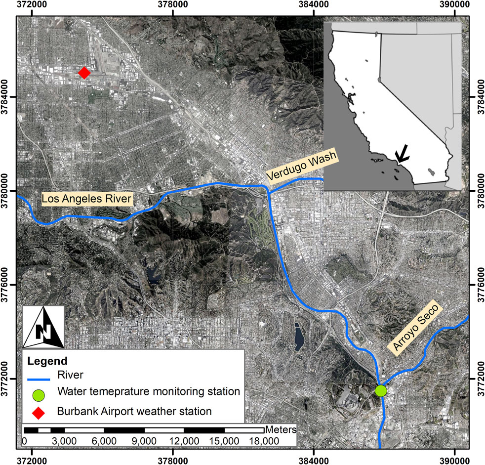
FIGURE 1. The study area in Los Angeles (LA) River, CA, showing the temperature monitoring station on LA River downstream of the Arroyo Seco tributary and Burbank Airport weather station location. The inset with an arrow shows the site location within the state of California.
We obtained LAR water temperature monitoring data for the study location from the Resource Conservation District of Santa Monica Mountains (Mongolo et al., 2017). Water temperature data were monitored from June through July 2016 using a combination of ONSET HOBO TidbiT v2 Water Temperature Data Loggers and HOBO Pendant Temperature Data Loggers (collectively, HOBOs) programmed to record time, date, and temperature (Mongolo et al., 2017). We obtained the meteorological data from the Burbank Airport weather station for the study period. After preparing water temperature and weather data (Figure 2), we pre-processed observed river temperature and weather data. Based on the available data for the monitoring station, we selected hourly data for the period June 10–July 18, 2016 (n = 936), during the dry weather (summer) period. The weather dataset had multiple features however only 12 features were monitored at hourly intervals. We cleaned and normalized the data based on the mean (μ) and standard deviation (σ) normalization method,

FIGURE 2. The schematic diagram of the steps for data gathering, cleaning, and organizing, as well as ML model's development and generating the predicted values based on the trained model to evaluate their performance.
In our machine learning model development, we followed 0.6, 0.2, and 0.2 ratios for the training, validation, and testing phases (Figure 2). Table 1 shows the overall statistical analysis of the selected features on the training and validation data before the normalization process. The training and validation phases were handled by the TensorFlow model using the Keras library capabilities. After obtaining satisfactory results in the validation period, we obtained predicted values, also using TensorFlow functions, to see the model’s performance compared to observed data. We analysed each machine learning model’s performance based on three factors including mean absolute error (
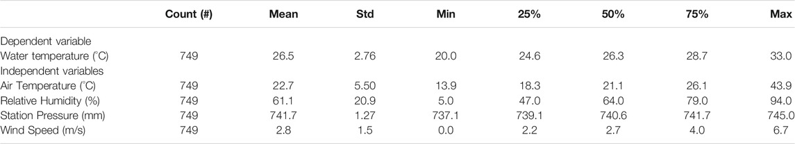
TABLE 1. Statistical characteristics of the dependent and independent variables have been used in the ML model development. In the table, “Std” stands for standard deviation.
Machine Learning Algorithms Development
In order to evaluate the performance of the DNNs1, we compared the trained models against single-layer and multilayer LR supervised machine learning models in the prediction process. For the single-layer model training, we used hourly air temperature as the predictive parameter and for the multilayer algorithms after applying feature engineering techniques, we selected hourly air temperature, relative humidity, station pressure, and wind speed as the independent variables for the period of June 10–July 18, 2016, for the training, validation, and testing phases (see Study Area and Inputs for more details). We considered the water temperature as the dependent variable for all the algorithms. For the training process, we trained the LR and DNN algorithms on Google’s TensorFlow model version 2.3.1 (Abadi et al., 2015) using Keras ANN library2 on Python 3.
LR model: For the LR learning algorithm, a single-variable and multilayer model was developed to predict water temperature from the input data. We used the Keras Sequential application programming interface (API) for predictions, which allow creating models layer-by-layer in a stepwise fashion. We defined a two-step sequence in building the models including 1) getting the normalized input date and 2) applying the linear transformation (y = β1x+β0) to produce the outputs using the Dense layer (i.e., regular deeply connected neural network layer). We set the term units in the Dense layer as 1 (layers.Dense(units = 1)) for generating the outputs. The variable units in the Dense layer represents the number of units and affects the output layer. The number of inputs is defined by the input_shape argument for the sequential model. We passed the air temperature input data as the single-layer model to develop a linear model with air temperature as the independent variable and water temperature as the dependent variable. For the multilayer model, in addition to air temperature, we added relative humidity, station pressure, and wind speed input data to the model for the training process.
In the LR with single-layer input, the model uses two trainable parameters including the intercept and slope of the line to obtain the best estimate of the linear model. In the linear equation,
where n is the number of target values for the training procedure.
After building the LR models, we compiled the model for training procedure configuration. We set the mean absolute error for the compilation’s loss function to be optimized based on the Adam optimization method (Kingma and Ba, 2014). Adam optimization is a stochastic gradient descent method (Ruder, 2016) that is based on adaptive estimation of first order and second-order moments. For the optimizer, we used learning rates ranging from 0.0001 to 10 with one order of magnitude in each round and selected the best one for each model. After testing the considered values, we selected the learning rate of 0.1 for the LR models and 0.001 for the DNN models. For the training phase, we set the number of epochs as 100 iterations. We kept 20% of the training data for unbiased validation. The validation set is not within the test set and 20% of the training data was used by the model for validation to provide more accurate results about the model’s improvement in the iterations. Splitting the data into train and test sets was random with a fixed seed for all the algorithms so the train-test splits were always deterministic and reproducible.
DNN model: By definition, a DNN is an ANN architecture with multiple layers between the input and output layers (Yu et al., 2016). To be consistent with the LR model training, we developed single-variable and multilayer DNN models to predict water temperature based on the input data using the Back-propagation technique (Keller, et al., 2016). We used the Keras Sequential API on normalized data for the prediction process and considered three sequences of steps in building the models including 1) getting the normalization input data layer, 2) applying two hidden, nonlinear Dense layers using the rectified linear unit (ReLU) nonlinear activation function (Jarrett et al., 2009), and 3) generating a single-output layer. We considered 64 neurons for each of the hidden layers using the Dense layer (Figure 3). The interior dense layers on ANN solutions are the regular deeply connected neural network layers and the name hidden for these additional DNN non-linear layers means that they are not directly connected to the inputs and outputs. Like the LR, we passed the air temperature time-series data to the single-layer DNN model to predict the water temperature. For the multilayer DNN model, in addition to the air temperature, we passed three other features including relative humidity, station pressure, and wind speed data. For the single-layer DNN model with two hidden layers, each with 64 neurons, the model used 4,353 trainable parameters, and for the multilayer DNN, with the same configuration, the model used 4,545 trainable parameters in the training phase.
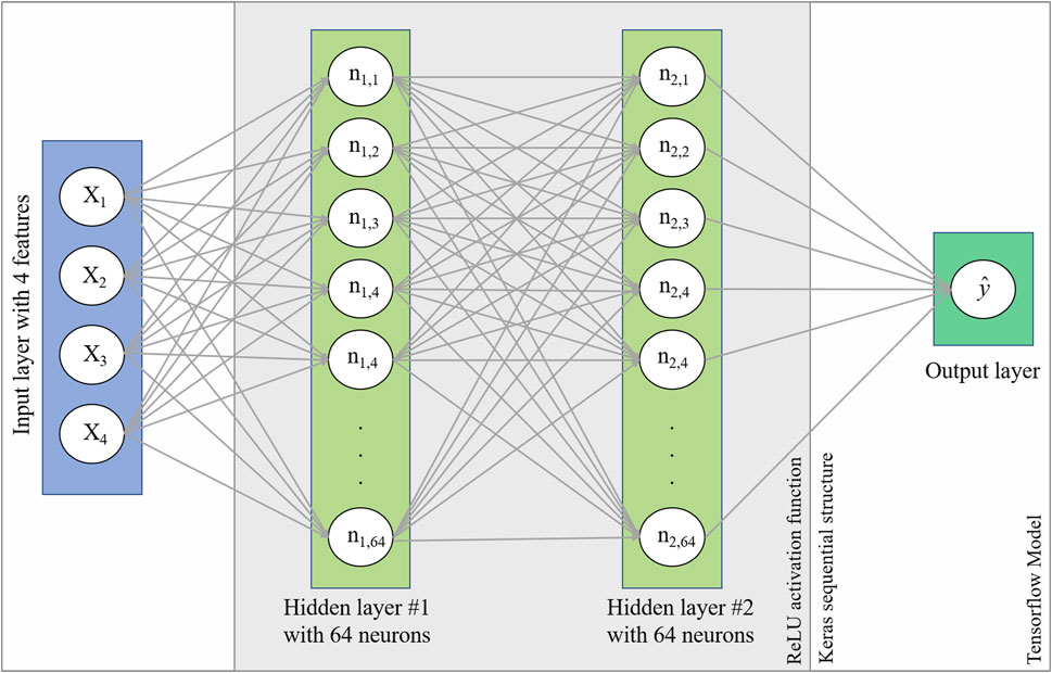
FIGURE 3. The multilayer DNN model structure with four features in the input layer, two hidden layers each with 64 neurons, and the output layer constructed using Keras library and implemented in TensorFlow model.
Just as we did in building the LR model, we compiled the DNN models for the training procedure. To keep the evaluation process similar between the LR algorithms and the DNN models, we considered the mean absolute error (MAE) for the compilation’s loss function to be optimized based on the Adam optimization method. In the training process, we set the number of epochs to be 100 and applied 20% of training data for the unbiased validation.
Results
By applying a single-variable LR to predict water temperature from air temperature, using the normalized data with 100 epochs, the average predicted water temperature was 26.9°C, 0.7°C higher than the average observed water temperature with a standard deviation of 1.7°C. Based on the loss function for the sequential model analysis, the optimizing parameter, the mean absolute error (MAE), dropped to 1.37°C after about 15 iterations in model training and stayed relatively constant for the rest of the iterations. The validation dataset loss optimized parameter, MAE, dropped to 1.23°C in the 15th iteration and stayed relatively constant for the rest of the simulations (Figure 4A). The training process based on a single feature made a linear relationship between the dependent and independent variables as shown in Figure 5A. The MAE for the testing process was 1.4°C (Table 2) and the R2 of the predicted and observed water temperatures was 0.68 (Figure 4B). Applying a two-sample t-test on the observed and predicted water temperature data showed that the p-value was 0.012 indicating 95% probability there was a significant difference between the two datasets (α = 0.05).
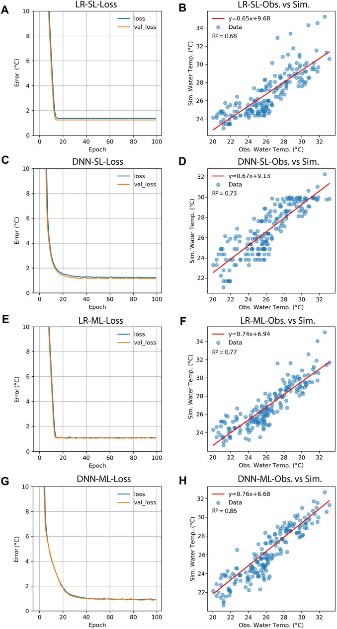
FIGURE 4. Model training and testing performance for four learning approaches including the linear regression (LR) and deep neural network (DNN) algorithms for single-layer (SL) and multiple layer (ML) conditions. Panels a, c, d, and g show the loss functions (MAE values) for the training and validation data sets and panels b, d, f, and h show the performance of the models in predicting the water temperatures.
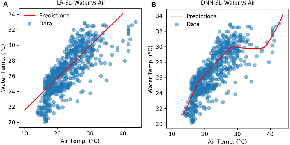
FIGURE 5. Scatter plots showing the relationship of the air and water temperature for the single-layer training approaches using the linear regression (A) and deep neural network (B) approaches. Panel b shows how the DNN model took the advantage the nonlinearity provided by the hidden layers.
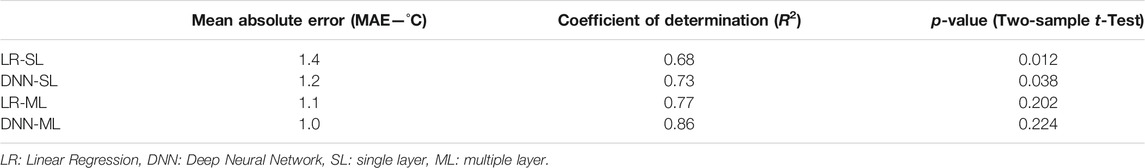
TABLE 2. Statistical analysis of four applied learning algorithms on TensorFlow model using the Keras library in the testing process.
We trained a DNN algorithm based on the single input normalized data, air temperature, and 100 epochs for predicting water temperature. The average predicted water temperature was 26.7°C, 0.5°C warmer than the average observed water temperature with a standard deviation of 1.6°C. The loss function of the DNN single input algorithm for the training and validation dataset showed a gradual decrease in the MAE variables. The MAE of the training dataset reached 1.26°C in iteration 83 and the validation dataset MAE was 1.15°C (Figure 4C). The DNN algorithm resulted in a non-linear relationship between the water and air temperature time series data (Figure 5B) showing that the DNN algorithm with two hidden layers and 4,353 trainable parameters could perform better in the training process. In the testing procedure, the algorithm’s MAE was 1.2°C, 14% better performance to the LR with the same number of inputs (Table 2). Comparing the observed and predicted water temperatures predicted by the DNN single layer algorithm, the R2 was 0.73, 7% better performance compared to the single-layer LR model (Figure 4D). However, the p-value for the two-sample t-test was 0.038 which was less than the α = 0.05 indicating that the observed and predicted water temperature datasets were significantly different with a probability of 95%.
By applying three additional features, relative humidity, station pressure, and wind speed, to the training process using the multivariate LR algorithm, the average predicted water temperature was calculated as 26.5°C, 0.3°C warmer than the average observed water temperature with a standard deviation of 1.4°C. Comparing the single input LR with the multiple-variable LR, the ∆T between the average observed and predicted water temperature improved by 0.4°C (57%) demonstrating that including additional features to the training process resulted in a significant improvement in the training process. The training and validation loss function optimized values, the MAEs dropped to 1.09°C and 1.02°C respectively after about 15 iterations of model training, and similar to the single input LR model, training stayed relatively constant to the end of the iterations (Figure 4E). The MAE for the testing process using this training approach was 1.1°C (Table 2) and the R2 for the predicted and observed water temperature datasets was 0.77, 13% more than the single-layer LR method (Figure 4F). By applying a two-sample t-test on the observed and predicted water temperature data we got a p-value of 0.201 indicating that assuming a probability of 95%, there was no significant difference between two datasets (α = 0.05) and two datasets were statistically similar.
Optimal performance was observed training a multivariate DNN model with two hidden non-linear layers with 4,545 trainable parameters. Similar to the multilayer LR, we included relative humidity, station pressure, and wind speed features to the training procedure. The average predicted water temperature was 25.4°C which was only 0.2°C higher than the average observed water temperature and the standard deviation was 1.2°C. Although compared to the multilayer LR, the ∆T was close, however, compared to the single-layer LR, there was 71% improvement in the ∆T. The loss function of the DNN multivariate algorithm for the training and validation dataset showed a gradually decreasing (similar to single-input DNN algorithm) in the MAE variables. The MAE of the training dataset reached 0.93°C after 100 iterations and the validation dataset MAE reached 0.88°C after 100 interactions in the optimizing process (Figure 4G). For the testing, the DNN algorithm provided an MAE 1.0°C, the lowest value among four training practices, which was 28% less than the MAE of the single-input LR (Table 2). Comparing the distribution of the absolute errors for the single-layer LR and multilayer DNN testing process showed that the DNN model’s absolute errors were 30% more below the 1°C threshold (Figure 6). The R2 value for the observed and predicted water temperature datasets with this algorithm, was 0.86, 26, and 12% higher compared to the single-layer LR and multivariate LR algorithms (Figure 4H). The p-value for the two-sample t-test was 0.224 which indicated that there was no significant difference between observed and predicted water temperature datasets considering a probability of 95%.
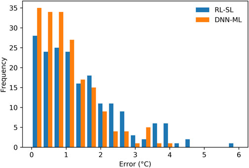
FIGURE 6. Histograms showing the absolute errors frequency distributions for the single-layer LR and multilayer DNN models in the testing process.
Discussion
Traditionally when observed data is not available, river water temperature has been predicted via air temperature using linear or non-linear relationships (Mohseni et al., 1998; Zhang and Johnson, 2017). Morrill et al. (2005) predicted river water temperature for 43 sites in the US and western Europe using LRs between the 7-days mean air and water temperatures and calculated an average root mean square error (RMSE) of 2.4°C. Morrill et al. (2005) also applied a non-linear regression equation (Mohseni et al., 1998) using air temperature data at 22 sites with the most comprehensive year-round coverage and got an average RMSE of 2.2°C for the sites. The non-linear regression equation proposed by Mohseni et al. (1998) has been used for generating the upstream river temperature boundary conditions for the mechanistic modelling of the water temperature simulations (Abdi et al., 2020; Sun et al., 2015) as an alternative when the observed data are not available. However, in dry weather simulations, Abdi and Endreny (2019) showed that the non-linear equation overestimated water temperature at the upstream boundary condition by about 1°C. Given that the upstream boundary temperature was considered as a sensitive parameter in temperature simulations (Abdi et al., 2020), overestimating that could cause overall warmer temperatures in the model. The machine learning-based multilayer models, specifically the DNN algorithms, could be a good alternative for the linear or non-linear regression equations for the cases when there are observed river temperature data for model training resulting in more accurate predictions. One application for the case study in this paper is predicting water temperature for the anadromous steelhead trout (Oncorhynchus mykiss) migration season, when observed data are not available. Stakeholders in the LAR aim to return a sustainable population of this sensitive cold-water native species in the LAR through stream restoration efforts. Using the multivariate DNN developed here, thermal conditions for the migration can be predicted in the absence of observed winter river temperatures; the DNN algorithm estimates the dependent (observed water temperature) with the independent (weather) data in dry weather conditions as inputs. We selected the epochs number based on Google’s general guidelines. Even though the computed error’s change after epoch 50 was almost negligible, we kept 100 epochs to present the pattern in the errors decrease for the applied algorithms. Since our dataset wasn’t large, the computations were fast. However, in practice and specifically working with large datasets, a smaller epoch number could be considered to avoid expensive computations.
River temperature data can be spatially and temporally sparse, yet it remains the master variable which controls the sustainability of fish, amphibians, and macroinvertebrates. River temperature influences the distribution of fish populations, their metabolism, their ability to spawn successfully, hatching, growth and survival. With climate change predicted to reduce thermal habitat for cold-water fish by 36 percent, and their populations by 50 percent (Mohseni et al., 2003), it is imperative to develop tools that are efficient and rely on few input variables to conserve thermal habitat for native species such as the steelhead trout (Benyahya et al., 2007). In areas where river temperature monitoring networks do not exist, or the data record is limited (similar to our case study with n = 936), the DNN algorithm can accurately infer river temperature from available weather data which will inform stream temperature standards in policy, help identify areas that need intervention to prioritize conservation, and enable entire river systems to be modelled. More efficient estimations of river temperature from the DNN algorithms will inform and improve models which may be used to predict changes in river temperature due to climate change, urbanization, dam removal and other river restoration efforts and depending on the objectives having a larger dataset could potentially increase the accuracy of the predictions.
Prior studies have tried to predict water temperature via ANN algorithms and concluded that even though air temperature is the most important predictor, including other attributes can improve prediction accuracy (e.g., Sahoo et al., 2009; DeWeber and Wagner, 2014; Piotrowski et al., 2015; Zhu et al., 2019); meaning that overall, multilayer machine learning algorithms could be better choices as we concluded in our analysis. The additional independent variables in these studies includes a wide range of descriptive properties which could affect water temperature directly or indirectly. For example, DeWeber and Wanger (2014) considered landform and landcover, Piotrowski et al. (2015) added current runoff and declination of the Sun, Sahoo et al. (2009) included solar radiation, and Zhu et al. (2019) included the day of the year, together with different forms of air temperature in their ANN analysis. Other studies (Isaak et al., 2010; Ruesch et al., 2012) have found that elevation can also be an effective independent variable for predicting water temperature. The current study is focused entirely on a highly urbanized area in a coastal area without much topographic relief, applying features related with the landform or landcover won’t make a significant improvement in the predictions in this region based on the feature engineering fundamentals. Furthermore, including elevation in the training analysis could decrease air temperature effects and downplay the impacts of increasing air temperatures under climate change (Stanton et al., 2012; DeWeber and Wanger, 2014). The range of the observed water temperature in the monitoring campaign (Mongolo et al., 2017) for the study area was 13.2°C between 20.0°C and 33.2°C in June and 8.0°C between 23.5°C and 31.5°C in July. The range of the predicted data using the multilayer DNN was 8.5°C between 21.7°C and 32.6°C, showing good performance with a reasonable load of computations. Our analysis confirmed that air temperature is the most important parameter impacting river water temperature and that including other features significantly improved results in our multilayer analysis. Including additional meteorological features would provide more robust predictions, specifically with climate change and urban heat island interactions and their impact on thermal fish habitat in urban landscapes (Kalnay and Cai, 2003).
Even though multilayer machine learning algorithms performed reasonably well in predicting LAR water temperature (Table 2), training the models for multiple climate conditions could generate more holistic machine learning-based predictors. Further, using long term observed data could be beneficial in the training/validation phases. For the LAR, the only available observed data were the monitored data provided by the Mongolo et al. (2017) for the dry weather period in 2016. Other observations are required for creating more robust mechanistic and/or machine learning-based models for predicting water temperatures. Longer observed time series data also could provide a good opportunity to apply other reliable deep learning methods such as long short-term memory (LSTM; Hochreiter et al., 1997) algorithm to assess its functionality in predicting water temperature as it is capable of learning long-term dependencies (Hochreiter et al., 2001) which could be useful in predicting water temperature time series data. Furthermore, future research on expanding the objectives of this study could focus on including additional predictive features such as direct and diffuse solar radiation, downloadable through the National Renewable Energy Laboratory’s National Solar Radiation Database (NREL NSRDB; Sengupta et al., 2018), and in-situ weather data. For this study we used weather data from nearby weather station data without including solar radiation data in order to make the data gathering process simple and easy to apply across other river systems and regions.
Conclusion
In this study we developed four machine learning-based models, single-layer and multilayer LR and DNN, to predict hourly river water temperature using meteorological data. We used an open-source TensorFlow model using Keras ANN library on Python 3 for our analysis and applied observed hourly water temperature as well as weather data from June 10 to July 18, 2016, for the training, validation (together, 80% of the data), and testing (20% of the data) processes. Air temperature was used as the independent variable for single-layer models and relative humidity, station pressure, and wind speed were considered as independent variables for the multilayer models. As supported by the literature, we found that air temperature was the most effective parameter in predicting water temperature, however, including additional features improved the predictions by 28% for the MAE and 26% for the R2 for the observed and predicted water temperatures, comparing the single-layer LR and multilayer DNN models. For two multilayer machine learning models both algorithms generated a p-value > α = 0.05 indicating no significant difference between observed and predicted water temperatures, the DNN model outperformed by 12% for their R2 values. These findings suggest that to predict water temperature, it is better to apply a range of machine learning algorithms and in some cases training the DNN models could be more challenging than the LR models. The overall modelling performances of the applied machine learning models in this study indicated that these models can be effectively used for river water temperature prediction in the absence of observed data. The machine learning models in this study are ultimately useful tools to address sustainable management of water resources and species conservation efforts. Findings from this work will assist hydrologic and earth systems modelers investigating alternative strategies for predicting water temperature specifically for determining upstream river temperature boundary conditions for mechanistic models.
Data Availability Statement
The raw data supporting the conclusion of this article will be made available by the authors, without undue reservation.
Author Contributions
Author contribution. Conceptualization, RA, AR, and TH; methodology, RA; software, RA; validation, RA and AR; formal analysis, RA; investigation, RA and AR; resources, RA, AR, TH; data curation, RA and AR; writing—original draft preparation, RA; writing—review and editing, RA, AR, and TH; visualization, RA; supervision, TH; project administration, TH.; funding acquisition, TH.
Funding
The funding was provided through interagency agreements (MOAs) from Los Angeles Department of Water and Power, City of Los Angeles Bureau of Sanitation, Los Angeles County Flood Control District, Los Angeles County Sanitation Districts.
Conflict of Interest
The authors declare that the research was conducted in the absence of any commercial or financial relationships that could be construed as a potential conflict of interest.
Publisher’s Note
All claims expressed in this article are solely those of the authors and do not necessarily represent those of their affiliated organizations, or those of the publisher, the editors and the reviewers. Any product that may be evaluated in this article, or claim that may be made by its manufacturer, is not guaranteed or endorsed by the publisher.
Acknowledgments
This project was conducted through a collaboration with the State Water Resources Control Board, the Los Angeles Regional Water Quality Control Board, and local municipalities and stakeholders. Principle funding was provided by the City of Los Angeles, Department of Water and Power (DWP) and Bureau of Sanitation (BoS). Additional funding was provided by Los Angeles County Public Works (LADPW), Los Angeles County Flood Sanitation Districts (LACSD), the Watershed Conservation Authority (WCA), a joint powers authority between the Rivers and Mountains Conservancy (RMC) and the Los Angeles County Flood Control District, and the Mountains Recreation and Conservation Authority (MRCA), a joint power of the Santa Monica Mountains Conservancy, the Conejo Recreation and Park District and the Ranch Simi Recreation and Park District. We thank Rosi Dagit, Resource Conservation District of Santa Monica Mountains, for providing us the observed temperature data. We thank our team members with Southern California Coastal Water Research Project (SCCWRP), all members of the Stakeholder Workgroup and the Technical Advisory Group who provided critical input, advice, and review over the course of this project. Additional project information is available at https://www.waterboards.ca.gov/water_issues/programs/larflows.html.
Supplementary Material
The Supplementary Material for this article can be found online at: https://www.frontiersin.org/articles/10.3389/fenvs.2021.738322/full#supplementary-material
Footnotes
1https://towardsdatascience.com/a-laymans-guide-to-deep-neural-networks-ddcea24847fb.
2Chollet. Software Available from https://keras.io/.
References
Abadi, M., Agarwal, A., Barham, P., Brevdo, E., Chen, Z., Citro, C., et al. (2015). TensorFlow: Large-Scale Machine Learning on Heterogeneous Systems. arXiv. Available at: https://arxiv.org/abs/1603.04467.
Abdi, R., and Endreny, T. (2019). A River Temperature Model to Assist Managers in Identifying Thermal Pollution Causes and Solutions. Water. 11 (5), 1060. doi:10.3390/w11051060
Abdi, R., Endreny, T., and Nowak, D. (2020). A Model to Integrate Urban River Thermal Cooling in River Restoration. J. Environ. Manage. 258, 110023. doi:10.1016/j.jenvman.2019.110023
Ahmadi-Nedushan, B., St-Hilaire, A., Ouarda, T. B. M. J., Bilodeau, L., Robichaud, É., Thiémonge, N., et al. (2007). Predicting River Water Temperatures Using Stochastic Models: Case Study of the Moisie River (Québec, Canada). Hydrol. Process. 21, 21–34. doi:10.1002/hyp.6353
Alizadeh, M. J., Kavianpour, M. R., Danesh, M., Adolf, J., Shamshirband, S., and Chau, K.-W. (2018). Effect of River Flow on the Quality of Estuarine and Coastal Waters Using Machine Learning Models. Eng. Appl. Comput. Fluid Mech. 12 (1), 810–823. doi:10.1080/19942060.2018.1528480
Allan, J. D., and Castillo, M. M. (2007). Stream Ecology. Dordrecht, Netherlands: Springer Science, Springer Netherlands. doi:10.1007/978-1-4020-5583-6
Aznar-Sánchez, J. A., Belmonte-Ureña, L. J., Velasco-Muñoz, J. F., and Manzano-Agugliaro, F. (2018). Economic Analysis of Sustainable Water Use: a Review of Worldwide Research. J. Clean. Prod. 198, 1120–1132. doi:10.1016/j.jclepro.2018.07.066
Benyahya, L., Caissie, D., St-HilaireOuarda, A. T. B. M. J., Ouarda, T. B. M. J., and Bobée, B. (2007). A Review of Statistical Water Temperature Models. Can. Water Resour. J. 32 (3), 179–192. doi:10.4296/cwrj3203179
Blockeel, H., Džeroski, S., and Grbović, J. (1999). Simultaneous Prediction of Multiple Chemical Parameters of River Water Quality with TILDE. Lecture Notes Computer Sci. (Including Subseries Lecture Notes Artif. Intelligence Lecture Notes Bioinformatics). 1704, 32–40. doi:10.1007/b72280
Bui, D. T., Khosravi, K., Tiefenbacher, J., Nguyen, H., and Kazakis, N. (2020). Improving Prediction of Water Quality Indices Using Novel Hybrid Machine-Learning Algorithms. Sci. Total Environ. 721, 137612. doi:10.1016/j.scitotenv.2020.137612
Chen, S. H., Jakeman, A. J., and Norton, J. P. (2008). Artificial Intelligence Techniques: An Introduction to Their Use for Modelling Environmental Systems. Mathematics Comput. Simulation. 78 (2–3), 379–400. doi:10.1016/j.matcom.2008.01.028
Dahl, T. E. (1990). Wetlands Losses in the United States: 1780’s to 1980’s. St. Petersburg, FL: Report to Congress. U.S. Fish and Wildlife Service. National Wetlands Inventory.
DeWeber, J. T., and Wagner, T. (2014). A Regional Neural Network Ensemble for Predicting Mean Daily River Water Temperature. J. Hydrol. 517, 187–200. doi:10.1016/j.jhydrol.2014.05.035
Díaz-Vico, D., Torres-Barran, A., Omari, A., and Dorronsoro, J. R. (2017). Deep Neural Networks for Wind and Solar Energy Prediction. Neural Process. Lett. 46 (3), 829–844. doi:10.1007/s11063-017-9613-7
Dogo, E. M., Nwulu, N. I., Twala, B., and Aigbavboa, C. (2019). A Survey of Machine Learning Methods Applied to Anomaly Detection on Drinking-Water Quality Data. Urban Water J. 16 (3), 235–248. doi:10.1080/1573062x.2019.1637002
Feigl, M., Lebiedzinski, K., Herrnegger, M., and Schulz, K. (2021). Machine-Learning Methods for Stream Water Temperature Prediction. Hydrol. Earth Syst. Sci. 25, 2951–2977. doi:10.5194/hess-25-2951-2021
Hadzima-Nyarko, M., Rabi, A., and Šperac, M. (2014). Implementation of Artificial Neural Networks in Modeling the Water-Air Temperature Relationship of the River Drava. Water Resour. Manage. 28 (5), 1379–1394. doi:10.1007/s11269-014-0557-7
Hochachka, P. W., and Somero, G. N. (2002). Biochemical Adaptation: Mechanism and Process in Physiological Evolution. Oxford: Oxford University Press
Hochreiter, S., Bengio, Y., Frasconi, P., and Schmidhuber, J. (2001). “Gradient Flow in Recurrent Nets: The Difficulty of Learning Long-Term Dependencies,” in A Field Guide to Dynamical. Editors S. C. Kremer, and J. F. Kolen.
Hochreiter, S., and Schmidhuber, J. (1997). Long Short-Term Memory. Neural Comput. 9 (8), 1735–1780. doi:10.1162/neco.1997.9.8.1735
Hu, X., Han, Y., Yu, B., Geng, Z., and Fan, J. (2020). Novel Leakage Detection and Water Loss Management of Urban Water Supply Network Using Multiscale Neural Networks. J. Clean. Prod. 278, 123611. doi:10.1016/j.jclepro.2020.123611
Isaak, D. J., Luce, C. H., Rieman, B. E., Nagel, D. E., Peterson, E. E., Horan, D. L., et al. (2010). Effects of Climate Change and Wildfire on Stream Temperatures and Salmonid Thermal Habitat in a Mountain River Network. Ecol. Appl. 20 (5), 1350–1371. doi:10.1890/09-0822.1
Isaak, D. J., Wenger, S. J., and Young, M. K. (2017). Big Biology Meets Microclimatology: Defining Thermal Niches of Ectotherms at Landscape Scales for Conservation Planning. Ecol. Appl. 27 (3), 977–990. doi:10.1002/eap.1501
Jarrett, K., Kavukcuoglu, K., Ranzato, M. A., and LeCun, Y. (2009). “What Is the Best Multi-Stage Architecture for Object Recognition,” in Proceedings of IEEE International Conference on Computer Vision (Kyoto, Japan: ICCV), 2146–2153.
Kalnay, E., and Cai, M. (2003). Impact of Urbanization and Land-Use Change on Climate. Nature. 423 (6939), 528–531. doi:10.1038/nature01675
Keller, J. M., Liu, D., and Fogel, D. B. (2016). Multilayer Neural Networks and Backpropagation. Fundamentals of Computational Intelligence: Neural Networks, Fuzzy Systems, and Evolutionary Computation. Piscataway, NJ, USA: IEEE, 35–60. doi:10.1002/9781119214403.ch3
Kingma, D. P., and Ba, J. L. (2014). Adam: A Method For Stochastic Optimization. arXiv. arXiv preprint: 1412.6980.
Krider, L. A., Magner, J. A., Perry, J., Vondracek, B., and Ferrington, L. C. (2013). Air-Water Temperature Relationships in the Trout Streams of Southeastern Minnesota's Carbonate-Sandstone Landscape. J. Am. Water Resour. Assoc. 49, 896–907. doi:10.1111/jawr.12046
Kumari, P., and Toshniwal, D. (2020). Extreme Gradient Boosting and Deep Neural Network Based Ensemble Learning Approach to Forecast Hourly Solar Irradiance. J. Clean. Prod. 279, 123285. doi:10.1016/j.jclepro.2020.123285
Lecun, Y., Bengio, Y., and Hinton, G. (2015). Deep Learning. Nature. 521 (7553), 436–444. doi:10.1038/nature14539
Miller, S. W., Wooster, D., and Li, J. (2012). Developmental Growth and Population Biomass Responses of River Dwelling Caddisfly to Irrigation Water Withdrawals. Hydrobiologia. 679, 187–203. doi:10.1007/s10750-011-0875-1
Mohseni, O., Stefan, H. G., and Eaton, J. G. (2003). Global Warming and Potential Changes in Fish Habitat in U.S. Streams. Climatic Change. 59, 389–409. doi:10.1023/a:1024847723344
Mohseni, O., Stefan, H. G., and Erickson, T. R. (1998). A Nonlinear Regression Model for Weekly Stream Temperatures. Water Resour. Res. 34 (10), 2685–2692. doi:10.1029/98wr01877
Mongolo, J., Trusso, N., Dagit, R., Aguilar, A., and Drill, S. L. (2017). A Longitudinal Temperature Profile of the Los Angeles River From June Through October 2016: Establishing a Baseline. Bull. South. Calif. Acad. Sci. 116, 174. doi:10.3160/soca-116-03-174-192.1
Morrill, J. C., Bales, R. C., and Conklin, M. H. (2005). Estimating Stream Temperature from Air Temperature: Implications for Future Water Quality. J. Environ. Eng. 131, 139–146. doi:10.1061/(asce)0733-9372(2005)131:1(139)
Muttil, N., and Chau, K. W. (2006). Neural Network and Genetic Programming for Modelling Coastal Algal Blooms. Int. J. Environ. Pollut. 28 (3/4), 223–238. doi:10.1504/ijep.2006.011208
Peterson, K. T., Sagan, V., Sidike, P., Hasenmueller, E. A., Sloan, J. J., and Knouft, J. H. (2019). Machine Learning-Based Ensemble Prediction of Water-Quality Variables Using Feature-Level and Decision-Level Fusion With Proximal Remote Sensing. Photogramm Eng. Remote Sensing. 85 (4), 269–280. doi:10.14358/pers.85.4.269
Piotrowski, A. P., Napiorkowski, M. J., Napiorkowski, J. J., and Osuch, M. (2015). Comparing Various Artificial Neural Network Types for Water Temperature Prediction in Rivers. J. Hydrol. 529 (P1), 302–315. doi:10.1016/j.jhydrol.2015.07.044
Poole, G. C., and Berman, C. H. (2001). An Ecological Perspective on In-Stream Temperature: Natural Heat Dynamics and Mechanisms of Human-Causedthermal Degradation. Environ. Manage. 27 (6), 787–802. doi:10.1007/s002670010188
Rabi, A., Hadzima-Nyarko, M., and Sperac, M. (2015). Modelling River Temperature from Air Temperature in the River Drava (Croatia). Hydrological Sci. J. 60, 1490–1507. doi:10.1080/02626667.2014.914215
Raffel, T. R., Rohr, J. R., Kiesecker, J. M., and Hudson, P. J. (2006). Negative Effects of Changing Temperature on Amphibian Immunity Under Field Conditions. Funct. Ecol. 20 (5), 819–828. doi:10.1111/j.1365-2435.2006.01159.x
Rigosi, A., Carey, C. C., Ibelings, B. W., and Brookes, J. D. (2014). The Interaction Between Climate Warming and Eutrophication to Promote Cyanobacteria Is Dependent on Trophic State and Varies Among Taxa. Limnol. Oceanogr. 59 (1), 99–114. doi:10.4319/lo.2014.59.1.0099
Rohr, J. R., and Raffel, T. R. (2010). Linking Global Climate and Temperature Variability to Widespread Amphibian Declines Putatively Caused by Disease. Proc. Natl. Acad. Sci. 107 (18), 8269–8274. doi:10.1073/pnas.0912883107
Ruder, S. (2016). An Overview of Gradient Descent Optimization Algorithms. arXiv preprint arXiv:1609.04747
Ruesch, A. S., Torgersen, C. E., Lawler, J. J., Olden, J. D., Peterson, E. E., Volk, C. J., et al. (2012). Projected Climate-Induced Habitat Loss for Salmonids in the John Day River Network, Oregon, U.S.A. Conservation Biol. 26 (5), 873–882. doi:10.1111/j.1523-1739.2012.01897.x
Sahoo, G. B., Schladow, S. G., and Reuter, J. E. (2009). Forecasting Stream Water Temperature Using Regression Analysis, Artificial Neural Network, and Chaotic Non-Linear Dynamic Models. J. Hydrol. 378 (3–4), 325–342. doi:10.1016/j.jhydrol.2009.09.037
Sattari, M. T., Apaydin, H., Band, S. S., Mosavi, A., and Prasad, R. (2021). Comparative Analysis of Kernel-Based Versus ANN and Deep Learning Methods in Monthly Reference Evapotranspiration Estimation. Hydrol. Earth Syst. Sci. 25, 603–618. doi:10.5194/hess-25-603-2021
Sengupta, M., Xie, Y., Lopez, A., Habte, A., Maclaurin, G., and Shelby, J. (2018). The National Solar Radiation Data Base (NSRDB). Renew. Sustainable Energ. Rev. 89, 51–60. doi:10.1016/j.rser.2018.03.003
Shin, Y., Smith, R., and Hwang, S. (2020). Development of Model Predictive Control System Using an Artificial Neural Network: A Case Study With a Distillation Column. J. Clean. Prod. 277, 124124. doi:10.1016/j.jclepro.2020.124124
Stanton, J. C., Pearson, R. G., Horning, N., Ersts, P., and Reşit Akçakaya, H. (2012). Combining Static and Dynamic Variables in Species Distribution Models Under Climate Change. Methods Ecol. Evol. 3 (2), 349–357. doi:10.1111/j.2041-210x.2011.00157.x
Sun, N., Yearsley, J., Voisin, N., and Lettenmaier, D. P. (2015). A Spatially Distributed Model For The Assessment Of Land Use Impacts On Stream Temperature In Small Urban Watersheds. Hydrol. Process. 29 (10), 2331–2345.
US Army Corps of Engineers (2016). HEC-RAS River Analysis System Hydraulic Reference Manual Version 5.0 CPD-68 US Army Corp of Engineers, Hydrologic engineering center, 960.
Todd, A. S., Coleman, M. A., Konowal, A. M., May, M. K., Johnson, S., Vieira, N. K. M., et al. (2008). Development of New Water Temperature Criteria to Protect Colorado's Fisheries. Fisheries. 33 (9), 433–443. doi:10.1577/1548-8446-33.9.433
Van Vliet, M. T. H., Yearsley, J. R., Franssen, W. H. P., Ludwig, F., Haddeland, I., Lettenmaier, D. P., et al. (2012). Coupled Daily Streamflow and Water Temperature Modelling in Large River Basins. Hydrol. Earth Syst. Sci. 16, 4303–4321. doi:10.5194/hess-16-4303-2012
Veról, A. P., Battemarco, B. P., Merlo, M. L., Machado, A. C. M., Haddad, A. N., and Miguez, M. G. (2019). The Urban River Restoration index (URRIX) - a Supportive Tool to Assess Fluvial Environment Improvement in Urban Flood Control Projects. J. Clean. Prod. 118058 (239), 1–14. doi:10.1016/j.jclepro.2019.118058
Wenger, S. J., Isaak, D. J., Luce, C. H., Neville, H. M., Fausch, K. D., Dunham, J. B., et al. (2011). Flow Regime, Temperature, and Biotic Interactions Drive Differential Declines of Trout Species Under Climate Change. Proc. Natl. Acad. Sci. 108 (34), 14175–14180. doi:10.1073/pnas.1103097108
Wilmer, P., Stone, G., and Johnston, I. (2000). Environmental Physiology of Animals. Oxford: Blackwell Science.
Yaseen, Z. M., Sulaiman, S. O., Deo, R. C., and Chau, K.-W. (2019). An Enhanced Extreme Learning Machine Model for River Flow Forecasting: State-Of-The-Art, Practical Applications in Water Resource Engineering Area and Future Research Direction. J. Hydrol. 569, 387–408. doi:10.1016/j.jhydrol.2018.11.069
Yu, D., Deng, L., Torsten, F., Seide, B., and Li, G. (2016). Discriminative Pretraining of Deep Neural Networks. US Patent Documents. US. 9, 235.
Zhang, Z., and Johnson, B. E. (2017). Hydrologic Engineering Center-River Analysis System (HEC-RAS) Water Temperature Models Developed for the Missouri River Recovery Management Plan and Environmental Impact Statement Environmental Laboratory, U.S. Army Engineer Research and Development Center, 120.
Zhang, K., Thé, J., Xie, G., and Yu, H. (2020). Multi-Step Ahead Forecasting of Regional Air Quality Using Spatial-Temporal Deep Neural Networks: A Case Study of Huaihai Economic Zone. J. Clean. Prod. 277, 123231. doi:10.1016/j.jclepro.2020.123231
Zhang, R., Wang, Y., Wang, K., Zhao, H., Xu, S., Mu, L., et al. (2019). An Evaluating Model for Smart Growth Plan Based on BP Neural Network and Set Pair Analysis. J. Clean. Prod. 226, 928–939. doi:10.1016/j.jclepro.2019.03.053
Zheng, A., and Casari, A. (2018). Feature Engineering for Machine Learning: Principles and Techniques for Data Scientists. 1st. ed. Sebastopol, CA, USA: O'Reilly Media, Inc.
Zhu, S., Nyarko, E. K., and Hadzima-Nyarko, M. (2018). Modelling Daily Water Temperature from Air Temperature for the Missouri River. PeerJ. 6 (6), e4894–19. doi:10.7717/peerj.4894
Keywords: water temperature, los angeles river, deep neural network, linear regression, mean absolute error
Citation: Abdi R, Rust A and Hogue TS (2021) Development of a Multilayer Deep Neural Network Model for Predicting Hourly River Water Temperature From Meteorological Data. Front. Environ. Sci. 9:738322. doi: 10.3389/fenvs.2021.738322
Received: 08 July 2021; Accepted: 14 September 2021;
Published: 28 September 2021.
Edited by:
Prosun Bhattacharya, Royal Institute of Technology, SwedenReviewed by:
Trista McKenzie, University of Gothenburg, SwedenShaukat Ali Mazari, Dawood University of Engineering and Technology, Pakistan
Copyright © 2021 Abdi, Rust and Hogue. This is an open-access article distributed under the terms of the Creative Commons Attribution License (CC BY). The use, distribution or reproduction in other forums is permitted, provided the original author(s) and the copyright owner(s) are credited and that the original publication in this journal is cited, in accordance with accepted academic practice. No use, distribution or reproduction is permitted which does not comply with these terms.
*Correspondence: Reza Abdi, rabdi@mines.edu