 Amélie Beucher
  Christoffer B. Rasmussen
 Thomas B. Moeslund2
 Mogens H. Greve
 - 1Department of Agroecology, Aarhus University, Tjele, Denmark
- 2Department of Department of Architecture, Design and Media Technology, Aalborg University, Aalborg, Denmark
Convolutional neural networks (CNNs) have been originally used for computer vision tasks, such as image classification. While several digital soil mapping studies have been assessing these deep learning algorithms for the prediction of soil properties, their potential for soil classification has not been explored yet. Moreover, the use of deep learning and neural networks in general has often raised concerns because of their presumed low interpretability (i.e., the black box pitfall). However, a recent and fast-developing sub-field of Artificial Intelligence (AI) called explainable AI (XAI) aims to clarify complex models such as CNNs in a systematic and interpretable manner. For example, it is possible to apply model-agnostic interpretation methods to extract interpretations from any machine learning model. In particular, SHAP (SHapley Additive exPlanations) is a method to explain individual predictions: SHAP values represent the contribution of a covariate to the final model predictions. The present study aimed at, first, evaluating the use of CNNs for the classification of potential acid sulfate soils located in the wetland areas of Jutland, Denmark (c. 6,500 km2), and second and most importantly, applying a model-agnostic interpretation method on the resulting CNN model. About 5,900 soil observations and 14 environmental covariates, including a digital elevation model and derived terrain attributes, were utilized as input data. The selected CNN model yielded slightly higher prediction accuracy than the random forest models which were using original or scaled covariates. These results can be explained by the use of a common variable selection method, namely recursive feature elimination, which was based on random forest and thus optimized the selection for this method. Notably, the SHAP method results enabled to clarify the CNN model predictions, in particular through the spatial interpretation of the most important covariates, which constitutes a crucial development for digital soil mapping.
1 Introduction
Digital soil mapping (DSM) techniques traditionally relate soil observations with point information extracted from different environmental covariates at corresponding locations. This representation of data as vectors at point location only partially describe a soil property or class. Taking into account spatial contextual information from covariates thus represents a crucial step forward for DSM and can be referred to as contextual mapping. During the last 2 decades, various studies attempted to incorporate spatial context through the preprocessing of environmental covariates. These original contextual mapping studies have used: different neighboring size to compute terrain attributes (Smith et al., 2006; Behrens et al., 2010b), adaptative filters applied on elevation data or derived attributes (Behrens et al., 2018b), covariates spatially transformed with wavelet analysis (Lark and Webster, 2001; Sun et al., 2017), hypercovariates created from elevation data (Behrens et al., 2010a; Behrens et al., 2014), and a multi-scale approach using aggregated covariates (Miller et al., 2015). All these studies relied on heavy preprocessing and/or subjective decisions concerning the resolution of covariates. Furthermore, Behrens et al. (2018a) compared different methods for multi-scaling analysis of terrain attributes combined to random forest with a deep neural network (DNN) algorithm (for clay and zinc content mapping). Other DSM studies investigated the use of DNNs for mapping soil moisture content (Song et al., 2016) and soil organic carbon content (Taghizadeh-Mehrjardi et al., 2020b; Emadi et al., 2020; Tao et al., 2020), identifying and delineating soil master horizons (Jiang et al., 2021), or spectral modelling (Singh and Kasana, 2019; Gholizadeh et al., 2020).
Within DNNs, convolutional neural networks (CNNs) represent a powerful and promising method for contextual mapping. CNNs have been originally used for computer vision tasks, such as image classification (Krizhevsky et al., 2012) and object detection. While the DNNs utilized in the aforementioned soil mapping studies use vector data extracted from covariates as input, CNNs use spatial contextual information extracted from covariates around each soil observation as input images (i.e., images or patches as xD arrays made of x covariates). Several DSM studies have been assessing CNNs for the mapping of soil organic carbon content (Padarian et al., 2019b; Wadoux et al., 2019; Wadoux, 2019), particle size fraction (Wadoux, 2019; Taghizadeh-Mehrjardi et al., 2020a), pH and nitrogen content (Wadoux, 2019), or for spectral modelling (Padarian et al., 2019c,a; Ng et al., 2019a,b; Xu et al., 2019; Pyo et al., 2020; Tsakiridis et al., 2020; Yang et al., 2020; Haghi et al., 2021; Zhong et al., 2021), but their potential for soil classification has not been investigated yet.
While DNNs provide high predictive power, their use almost systematically raise concerns because of their presumed low interpretability (i.e. the black box pitfall; Samek et al. (2019); Khaledian and Miller (2020)). However, a recent sub-field of Artificial Intelligence (AI) called explainable AI (XAI) focuses on clarifying complex AI models, such as DNNs, in a systematic and interpretable manner (Samek et al., 2019). For instance, it is possible to apply model-agnostic interpretation methods (Molnar, 2021) to enable extracting interpretations from any machine learning model. In particular, SHapley Additive exPlanations (SHAP) developed by Lundberg and Lee (2017) constitute a method to explain individual predictions, SHAP values representing the contribution of a covariate to the final model predictions. As of today, one DSM study (Padarian et al., 2020) evaluated the use of SHAP for interpreting the predictions of a CNN model, in particular in the geographical space, while two other DSM studies used SHAP to interpret spectral models (Haghi et al., 2021; Zhong et al., 2021).
During the last decade, a few classical DSM methods were evaluated for mapping acid sulfate (AS) soils at different extents. Clustering through fuzzy k-means was tested to map coastal AS soils on a field extent in Australia (Huang et al., 2014a,b). Fuzzy logic was used to generate a preliminary map for AS soil occurrence at regional extent in Finland (Beucher et al., 2014). Artificial Neural Networks (ANNs) were assessed to map AS soil occurrence and several soil properties characterising the related environmental risks at catchment extent in southwestern Finland (Beucher et al., 2013, 2015). ANNs were also evaluated to map potential AS soils in the wetland areas of Jutland, Denmark (Beucher et al., 2017).
The present study will evaluate the use of CNNs for the classification of potential AS located in the wetland areas of Jutland, Denmark (c. 6,500 km2). The two main objectives are, firstly, to assess the use of CNNs in comparison with random forest for AS soil classification, and secondly and most importantly, to apply a model-agnostic interpretation method to clarify the final model predictions.
2 Material and Methods
2.1 Study Area
The wetlands located over Jutland, the continental part of Denmark, constitute the study area (Figure 1). They cover about 6,500 km2 and represent approximately 20% of the Jutland peninsula (Madsen et al., 1985). Wetlands are saturated soils, such as histosols, fluvisols and gleysols (IUSS Working Group WRB, 2006). These areas were mainly used for hay production until the second half of the 19th century when tile drainage was introduced (Greve et al., 2014). Most of the wetlands (c. 5,100 km2) have been artificially drained and intensively farmed, the main crop being cereals and grass (Bou Kheir et al., 2010). Low-relief sandy glaciofluvial outwash plains from the Weichselian glaciation (i.e., Last Glacial Maximum) dominate in the western part of the study area (c. 1,200 km2). These plains area surrounded by slightly protruding islands of older and strongly eroded moraine landforms from the Saalian glaciation (c. 700 km2) (Madsen et al., 1985; Madsen and Jensen, 1988). The eastern part of the study area consists of Weichselian moraine landforms (c. 900 km2) while the northern part is composed of late- and post-glacial marine sediments (c. 2,400 km2) (Madsen and Jensen, 1988). Cretaceous limestone dominates in northern Jutland and Djursland. Tertiary mica-rich sand and clay prevail in the rest of Jutland (Madsen and Jensen, 1988). The study area has a temperate climate. The mean temperature is 0°C in the winter and 16°C in the summer. The average annual precipitation is about 800 mm in central Jutland (Danmarks Meteorologiske Institut, 1998).
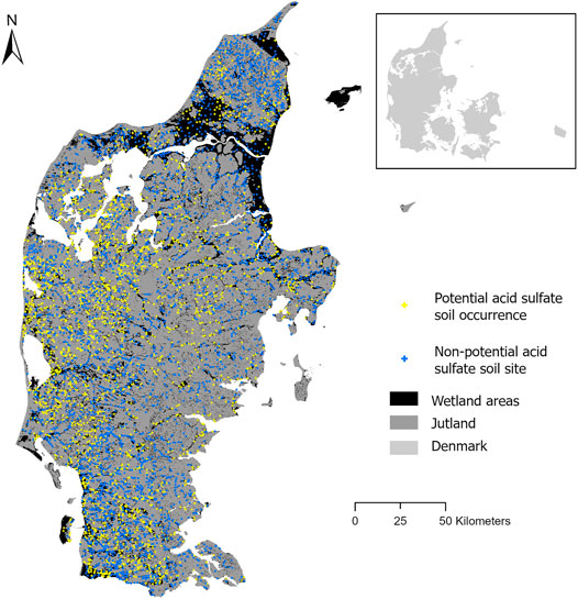
FIGURE 1. Distribution of the soil observations in the study area.
2.2 Soil Observations
Soil observations were extracted from the Ochre Classification database which resulted from the potential AS soil mapping conducted in the 1980s (Madsen et al., 1985). Soils in wetland areas were targeted and surveyed through conventional mapping. Field work was carried out from May to October over a 3-year period (1981–83). The original selection of about 8,000 sampling sites was based on historical topographic maps, geological maps, soil maps and maps from previous moorland studies, representing an even distribution in wetlands and soil types (Madsen et al., 1985). The carbonate-free samples were considered as potential AS soils if their pH dropped below 3.0 within 16 weeks of incubation at room temperature (Madsen et al., 1985). For samples containing calcium carbonates, the acid-neutralizing capacity (ANC) was calculated from calcium and magnesium concentrations. The samples were classified as potential AS soils if the calculated ANC was smaller than the amount of sulfuric acid potentially produced by the oxidation of the pyrite contained in the sample (Madsen et al., 1985). A subset of 5,885 points was selected to be used in the present study as the original set included points which were incorrectly classified. The main misclassification concerned points displaying a minimum incubation pH between 3.1 and 4.0 and wrongly classified as potential AS soils. For more details concerning the soil observations and their classification, we refer the reader to Beucher et al. (2017). A binary classification was used within the present study: potential AS soil occurrences (n = 2,309) and non-potential AS soil sites (i.e. soils which are not and will not become AS soils; n = 3,576) (Figure 1).
2.3 Environmental Data and Variable Selection
For the present study, the available 23 gridded environmental data can be divided into three groups: topography (21 covariates), soil (1 covariates) and climate (1 covariate). Danish variables typically have a 30.4-m resolution because the digital elevation model (DEM) was originally derived from the 1.6-m resolution national airborne LiDAR (Light Detection and Ranging) data and resampled to 30.4-m resolution (Adhikari et al., 2014). Variable selection was employed in order to follow the principle of parsimony (i.e., Occam’s razor) which indicates that a better model can explain the same phenomena from fewer variables (Batty and Torrens, 2001). Moreover, using fewer covariates may ease result interpretation and enable faster computer processing (Brungard et al., 2015). Recursive feature elimination (RFE) was applied using the R package caret (Kuhn, 2021) to select the optimal set of covariates for modelling based on the random forest (RF) algorithm (R Core Team, 2021; Cai et al., 2018). First, a RF model was trained on all 23 gridded environmental data, yielding the importance of each covariate. Then, the least important covariates were removed. This was recursively done until the optimal number of covariates is reached. The optimal number of covariates is defined through cross-validation. RFE analysis was carried out with the following tuning parameters: the number of tested environmental covariates (mtry) at each split as default and the number of trees (ntree) at 1,000. Finally, 14 environmental covariates were selected and utilized as input data for further modelling (Table 1). Among them, 10 terrain attributes were derived from the DEM within ArcGIS (ESRI, 2020) or SAGA (System of Automated Geoscientific Analyses) GIS (Conrad et al., 2015).
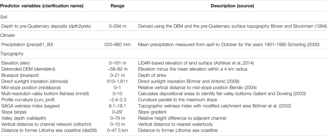
TABLE 1. Environmental covariates selected for the modelling.
2.4 Random Forest and Scaled Environmental Data
Random forest (RF) is used as a reference modelling technique for comparison with the CNN approach. RF is a tree-based ensemble method which has been widely used in digital soil mapping studies to carry out classification and regression predictions (Hengl et al., 2018). In this study, RF tuning parameters such as ntree (the number of trees) and mtry (the number of input environmental covariates in each random subset), were determined using a Bayesian optimization procedure within R with packages ranger (Wright and Ziegler, 2017) and rBayesianOptimization (Yan, 2021). Bayesian optimization constitutes a sequential model-based optimization procedure that enables the identification of the optimum internal parameters of models in a more efficient way than grid, random or manual (i.e., trial-and-error) search (Hinz et al., 2018). Within Bayesian optimization, the unknown objective function is considered as a random function defined by a prior probability distribution. Using function evaluations as data, the prior is updated to form the objective function posterior distribution. The posterior distribution is in turn used to determines the next evaluation point. Both CNN and RF models utilized this optimization procedure, as well as the same calibration and test sets. Smoothing mean filters with different neighbourhood sizes (i.e., 1, 3, 5, 7, 9, 15, 21, and 29 pixels) were used to provide the RF models with scaled versions of the original environmental covariates, in an attempt to achieve a fairer comparison between CNN and RF (Taghizadeh-Mehrjardi et al., 2020a). RF models were thus trained both with the original 14 selected environmental covariates and the scaled versions of this selection (i.e., 112 covariates in total). Smoothing mean filters constitute a common technique to derive scaled versions of environmental data in digital soil mapping studies (Grinand et al., 2008; Behrens et al., 2010a; Behrens et al., 2010b). Mean filtering consists in replacing each pixel value in an image with the mean (i.e., average) value of its neighbours, including itself (Shapiro, 1970; Boyle and Thomas, 1988). The R package raster (Hijmans, 2021) was used for filtering the original environmental covariates.
2.5 Convolutional Neural Networks
2.5.1 General
A Convolutional Neural Network (CNN) used for classification or regressions tasks can be divided in two parts: the first part consists in convolutional filtering for hierarchical feature extraction and the second part comprises fully-connected layers of neurons which calculate an output value, finalising the classification or regression task. This second part is equivalent to a classical ANN. Feature extraction by convolutional filtering is carried out through different convolution and pooling steps or layers that can be repeated several times. The objective of this first step is to extract the most relevant features and the multiple representations of the spatial scales from the x environmental covariates fed as an input xD array or patch (equivalent to an image) to the CNN (Taghizadeh-Mehrjardi et al., 2020a). The first convolutional layers extract low-level features or small local patterns (i.e., edges and corners) while the last convolutional layers extract high-level features, such as image structures (Mahdianpari et al., 2018). CNNs can also be more complex and include additional parts for more complex tasks, such as object detection.
A convolution layer consists in a filtering stage and the application of an activation function. This layer is defined by the convolutional filter size and the number of filters which represents the depth of the output feature map produced by the convolutional layer (Mahdianpari et al., 2018). A filter or moving window with typical sizes of 3 × 3 or 5 × 5 pixels progresses over the input xD array or patch (from left to right and from top to bottom). The values of the filter represent the weights for each pixel. These filter weights are randomly initialised and adjusted by backpropagation which is a common algorithm in the training of feed-forward neural networks. Typically, an optimizer, such as stochastic gradient descent or ADAM, supports backpropagation. Specifically, this algorithm computes the gradient of the loss function using the weights of the model for a particular input and output. The filter weights are first multiplied by the overlapping pixel values of the input patch. Then, they are all summed up to a new output value which is assigned to the center location of the filter. The area of input patch which is overlaid by the filter is called receptive field. As the filter progressively moves over the input image, a new feature map is formed, constituting a combination of all environmental covariates. For comparison, the filter weights for all pixels of a feature map are the same in a CNN while each neuron has its own set of weights in a classical ANN. Applying different filter weights enables the identification of distinct specific spatial properties within the input data.
A convolution step can be carried out several times. While the first convolution is applied to the original input patch (i.e., made from the original set of environmental covariates), the following convolution steps are applied to the previously generated feature maps, creating more generalized and spatially coarser levels of information. The size of the convolution filter and the stride control the generation of convoluted feature maps in a CNN. A stride is the step width used by the filter to progress over the input image. For example, a stride of 2 implies that only every second pixel is considered and every other is skipped, which results in a reduced size of the feature maps. A convolution step is followed by a transformation or calculation step through the use of an activation function. This activation function represents a mathematical non-linear transformation function which determines the relationship between input values and output value. It calculates the output value of a neuron by non-linearly transforming the weighted sum of the input value, and passes this output to the next layer in the network. The rectified linear unit (i.e. ReLU) constitutes a commonly used nonlinear activation function for deep learning.
A pooling layer constitutes a resampling or filtering step where kernel sizes of 2 × 2 pixels and a stride of 2 are generally used. By reducing the number of pixels in feature maps, the spatial dimensions and computation costs are also minimised in order to avoid overfitting and further generalize the information. The maximum value within the kernel is selected when using the max-pooling operator.
Convolution and pooling steps constitute the shared layers in a CNN and are followed by the fully-connected network layers. A flattening step enables the transition from the shared layers into a fully-connected network (i.e., single-pixel feature maps transformed into feature vectors to be used as input within the fully-connected network). Within the second part of a CNN, the extracted spatially local features from the shared layers are basically combined. A main difference between the shared layers and the fully-connected layers is that the neurons in a convolution layer are only connected to the neurons in the receptive field and not to all the neurons in the previous layer. In order to avoid or reduce overfitting, a technique called dropout can be used within the shared layers and the fully-connected network (Krizhevsky et al., 2012). Dropout randomly mutes neurons during the training phase.
2.5.2 Input Data Augmentation
In addition to dropout, data augmentation enables to further avoid overfitting problems (Krizhevsky et al., 2012). Data augmentation generates more training samples from the available training data using a number of possible transformations without changing its meaning (Simard et al., 2003). For example, the original training data can be rotated by 90°, 180°and 270°, increasing the number of training samples. The main goal is to enable the model to explore more aspects of the training samples and, thus to increase the generalization ability of the CNN. This is crucial as the prediction ability of a CNN greatly depends on the amount of the existing training samples (Krizhevsky et al., 2012).
2.5.3 CNN Architecture Selection and Parameter Optimization
The architecture of the CNN model used in the present study and its specifications are represented in Figure 2. All environmental covariates were preprocessed through standardization (i.e., centred on 0 and scaled to a standard deviation of 1). An optimal window size for model training was determined by testing various sizes of 3, 5, 7, 9, 15, 21, and 29 pixels for the prediction of potential AS soil occurrence. Importantly, Bayesian optimization was used to identify the optimal network hyperparameters (Hinz et al., 2018). In this study, the number of filters and neurons, filter size, max-pooling kernel size, learning rate (i.e., how many weights are updated during training), dropout rate, activation function and optimizer were determined using Bayesian optimization with 60 iterations. This optimization algorithm employs an objective function (in our case, the overall accuracy) to train a model through a Gaussian process using training samples as input. Different network depths (i.e., number of layers within the CNN model) were also tested. The simple architecture presented in Figure 2 was selected as the increase in accuracy yielded by more complex models was not substantial. The selected model includes a sequence of shared layers: first, a convolutional layer with a filter size of 3 × 3 and a ReLu activation function, second, a max-pooling layer with a size of 2 × 2, third, a dropout layer which randomly disconnects 15% of the connections in order to prevent overfitting, and fourth, a flatten layer. The flatten layer enables the connection between the shared layers and the succeeding fully-connected layers by converting matrices into vectors. The fully-connected layers performs the classification part of the CNN, receiving information from the previous layers to generate predictions (Taghizadeh-Mehrjardi et al., 2020b).
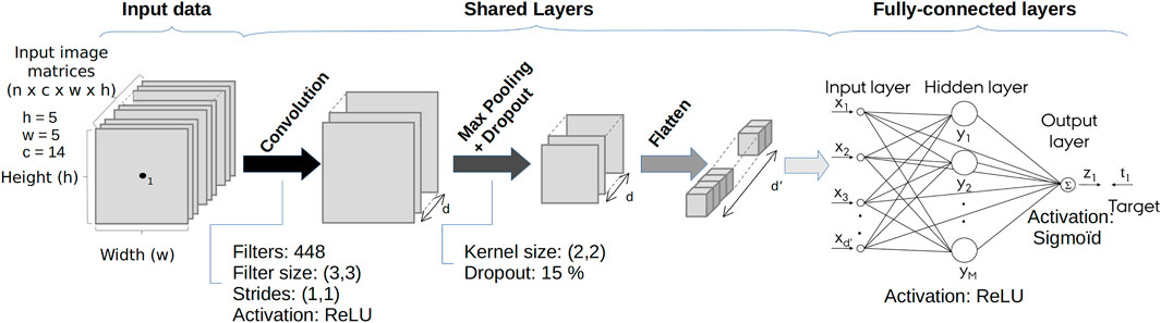
FIGURE 2. Architecture of the selected CNN.
CNNs were implemented in Python (v3.8) (Python Software Foundation, 2021) using Tensorflow/Keras (v2.6) (Abadi et al., 2016; Keras, 2021) and Tensorboard (v2.6). The experiments were carried out on an Intel CPU i7-8,700 machine with 3.2 GHz 6-core CPU and 32 GB RAM memory with a Nvidia GeForce RTX 2070 GPU under CUDA version 11.4.
2.5.4 Training, Validation and Test Datasets
In order to evaluate the performance of our CNN models to predict potential AS soils, 75 and 25% were randomly selected as training and test dataset, respectively. On the remaining 75%, data augmentation was carried out to increase the amount of the training samples. Additionally, to find the optimal hyperparameters and to avoid overfitting, we used a random subset (80 and 20%) of the augmented data for training and validation of the CNN. The test dataset (25%), which is independent of the training and validation samples, is used to estimate the generalisation error of the proposed CNN and used for the final model comparison (i.e., between RF and CNN). The relationship between observed and predicted points for the training and validation data sets was evaluated with the overall prediction accuracy (OA) which represents the number of correctly classified points divided by the total number of points.
2.6 Interpretability With SHAP
SHAP (SHapley Additive exPlanations) constitutes a method based on Shapley values that enables explaining individual predictions (Lundberg and Lee, 2017). Within a game theory context, each feature (or covariate) value can be defined as a player in a coalitional game (i.e., a modelling task) where the prediction represents the payout. Shapley values are used to estimate how the payout is distributed among the covariates (Molnar, 2021). In order to compute Shapley values, two models are fitted for a covariate i: one fS∪{i} including the covariate i and another fS withholding it. The difference between the predictions of the two models on the current input x, fS∪{i}(xS∪{i}) − fS (xS), constitutes the specific contribution of covariate i (Lundberg and Lee, 2017). Since the specific contribution of a covariate depends on the other utilised covariates, the preceding calculation is computed for all the possible covariate subsets S ⊆ F, where F is the set of all covariates. The overall covariate contribution ϕi represents the weighted average of all specific contributions as follows:
The SHAP method defined by Lundberg and Lee (2017) adapts the procedure described above by applying sampling approximations to Eq. 1 and approximating the effect of removing a covariate by using other samples from the training dataset. In short, a SHAP value indicates the relative contribution, positive or negative, of a covariate in a given sample to the model’s output (Zhong et al., 2021). Moreover, Lundberg and Lee (2017) developed a Deep SHAP explainer (DeepExplainer) to compute SHAP values specifically for DNNs. The method applies linear approximations which are aggregated by using a composition rule enabling the approximation of SHAP values for the whole model. Basically, in order to explain a complex original model f, we use an explanation model g simpler than the original. The explanation model is also based on simplified inputs x′ which map to the original inputs x through a mapping function x = hx (x′) (Lundberg and Lee, 2017). This local method try to ensure that g (z′) ≈ f (hx (z′)) when z′ ≈ x′. In order to assess the effect of varying the input x, z′ is defined from reference values sampled from observations from the training dataset (Padarian et al., 2020). The contribution ϕi of each covariate (Eq. 1) is then included in a linear function of binary variables (i.e., an explainable variable being either present, 1, or absent, 0):
where z′ ∈ {0,1}M, M is the number of simplified input features, and
The Deep SHAP Explainer is included in the SHAP Python library (Lundberg and Lee, 2017) and was used for CNN interpretability purposes. Deep SHAP supports both TensorFlow and Keras models by extending the DeepLIFT algorithm from (Shrikumar et al., 2017) using a distribution of background samples to calculate SHAP values for the selected network. The data utilized to perform the approximations correspond to the CNN training dataset. In order to confirm that the model is capturing sensible relationships between the class target (i.e., potential AS soil occurrence) and the environmental covariates, we applied SHAP to visualize the distribution of the main contributing environmental covariates over the whole study area, both as a map and as a histogram. We also focused on a selection of main contributing environmental covariates and inspected their distribution as a single layer over the study area.
3 Results and Discussion
3.1 RF Models
The predictive classification abilities of RF were evaluated for the classification of potential AS soil occurrence in the wetlands of Jutland. RF models were tested using firstly, the 14 environmental covariates selected with RFE, and secondly, the 112 scaled covariates for which smoothing mean filters were utilized. Based on the Bayesian optimization procedure, the optimal RF tuning parameters were defined for each RF model. The RF model built with the original 14 covariates (RForiginal) used a random subset size of 10, a minimal nodesize of 5 and a tree size of 1,600 while the RF model developed with the scaled covariates (RFscaled) used a random subset size of 5, a minimal nodesize of 3 and a tree size of 680. Both models used the Gini splitting rule. RForiginal and RFscaled models yielded comparable OA values for validation, 61 and 63%, respectively. These results indicate that the RFscaled model did not seem to use the contextual spatial information to classify potential AS soils more accurately than the RForiginal model. For the RForiginal model, the most important variables were elevation, depth to pre-Quaternary deposits, detrended elevation model and mid-slope position. For the RFscaled model, they were elevation and detrended elevation model at different scales (fine first, then coarse). AS soils occur in low-lying areas which supports the importance of elevation layers. The depth to pre-Quaternary deposits also represents a useful covariate in particular for central and southern Jutland where potential AS soils can form in non-marine environments (i.e. glaciofluvial outwash plains and moraine landforms) overlaying pyrite-containing Tertiary sediments (Beucher et al., 2017).
3.2 CNN Models
Using Bayesian optimization, the optimal hyperparameter values were selected for our CNN models. Considering the CNN model yielding the highest OA (68%), the hyperparameters were: ReLU as activation function, ADAM as optimizer, binary cross entropy as loss function, a learning rate of 0.001, a convolution filter size of 3 × 3 and 448 filters, a max-pooling kernel size of 2 × 2, and a dropout rate of 15%. This model also used augmented data. However, the CNN model with similar architecture and parameters based on data without augmentation already yielded a comparable OA value (63%). The optimal patch size for training our CNN models was determined by assessing different sizes (i.e. 3, 5, 7, 9, 15, 21, and 29) for the classification of potential AS soils. An increase in patch size up to 5 increases OA which then decreases from the patch size of 9. A patch size of 5 was thus found to be optimal. Considering the spatial resolution of covariates of 30.4 m, a patch of 5 × 5 includes the contextual information of approximately 76 m (i.e., 5/2 × 30.4 = 76 m). Therefore, the contextual information of environmental covariates within a 76 m radius was demonstrated as valuable for classifying potential AS soils compared to the local information usually used at a specific point. This result is in line with findings of past studies (Behrens et al., 2010a; Behrens et al., 2010b; Behrens et al., 2018a; Behrens et al., 2018b; Padarian et al., 2019b; Wadoux et al., 2019), which reported that the prediction accuracy increased by including contextual information within the modelling.
3.3 CNN/RF Model Comparison
The best performing CNN model yielded a slightly higher OA than both RF models, improving the prediction by 5 and 7% compared to RFscaled and RForiginal models, respectively. This relatively small difference in performance can might be explained by the use of RFE as a common variable selection method. For this study, RFE was based on the RF algorithm and thus rendered a selection of covariates optimized for this method. As indicated by Brungard et al. (2015), the use of RF within RFE most likely explains the consistent higher accuracies rendered by RF models in comparison with other models. Even though ANNs in general, and CNNs in particular, have the ability to extract relevant information from large datasets (Gershenfeld, 1999; Chagas et al., 2013) and generalize from relatively imprecise data (Porwal et al., 2003), variable selection might constitute an important processing step when implementing them. Moreover, a variable selection optimized for RF, a method resistant both to noise (Strobl et al., 2007) and multicollinearity (Hengl et al., 2018), might not be the most sound option for CNNs. However, the use of a specific variable selection method for CNNs might also yield a different selection of covariates, which would hinder comparing the two methods. Another possible most probable reason for the comparable performances of RF and CNN lies in is the relatively coarse spatial resolution of the environmental covariates used as input data, which might may have represented a strong limitation for the CNN models. As stated previously using a patch of 5 × 5 with 30.4-m resolution covariates resulted in the use of contextual information within a 76-m radius around soil observations for the training of CNN models. Employing covariates with a finer resolution, for example 10 m, would enable to use larger size patches and thus feed the CNN models with more details to investigate in each input image. Moreover, this limitation due to the resolution could also explain the fact that CNN models with more complex architectures did not yield notable increases in accuracy compared to the simple CNN selected in this study (Figure 2). While the first convolution layer is applied to the input environmental covariates and extracts low-level features, the following convolution layers are applied to the created feature maps and thus, produce more generalized and spatially coarser level of information. In our case, the additional convolution layers might only have extracted coarser information from coarse input data, which did not enable the fully-connected layers to generate more accurate predictions.
Comparing the prediction maps in Figure 3, both models predicted high probability areas located along the western coast of Jutland, for example the delta region of the Skjern River (i.e. the bottom located close-up in Figure 3) which constitutes a well-known potential AS soil area (Madsen and Jensen, 1988). However, the RF model tended to over-predict mid-range values (Figure 4), which can be observed in the northern part of Jutland, in particular in the top-located close-up in Figure 3. This can be interpreted as RF poorly generalizing from input data. In comparison, the CNN model over-predicted low probability values (Figure 4), which can be explained by the fact that the set of non-potential AS soils (n = 3,576) is larger than the one of potential AS soils (n = 2,309).
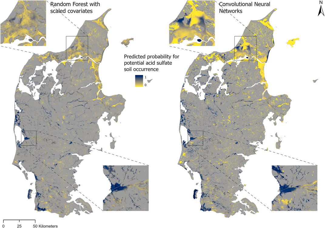
FIGURE 3. Maps of the predicted probability for potential acid sulfate soil occurrence generated using Random Forest (RF) with scaled covariates (left) and Convolutional Neural Networks (CNN; right).
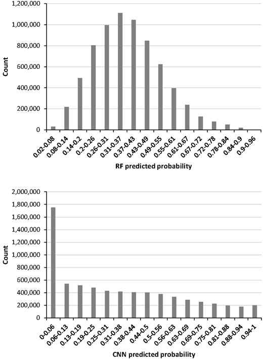
FIGURE 4. Distribution of the predicted probability for potential acid sulfate soil occurrence generated using Random Forest (RF) with scaled covariates (top) and Convolutional Neural Networks (CNN; bottom).
3.4 Interpretability Using SHAP
In order to compute SHAP values, we used 200 training points from each class as background data (i.e., data to perform the approximations). These values were found empirically as it was determined to give a good trade-off between consistency of SHAP values and computation time since the computation of SHAP values from the explainer increases linearly with the number of samples (i.e., training points).
In order to gain more insight as to the spatial interpretation of the model over Jutland, the most important covariates are displayed in Figure 5. The map shows the spatial distribution of the covariates with the largest SHAP value for each 5 × 5 patch, meaning the largest positive or negative deviation from the baseline SHAP values calculated from the background samples. Moreover, Figure 6 shows the distribution of the covariates with the largest SHAP contribution for each patch. Figure 6 indicates that the detrended DEM, depth to pre-Quaternary deposits and distance to Littorina sea coastline constitute the most important covariates in terms of occurrence, followed by the multi-resolution valley bottom flatness and precipitation. Figure 5 shows that the detrended DEM is the most important covariate in wetland areas all over Jutland, which can be expected as soils typically occur in low-lying areas. The depth to pre-Quaternary deposits represents the second most important covariate, occurring mostly in the western half of Jutland. This can be explained by the fact that potential AS soils can form in non-marine environments (i.e., in glaciofluvial outwash plains and moraine landforms as seen in Figure 7) overlaying pyrite-rich Tertiary sediments (Beucher et al., 2017). The distance to the former Littorina sea coastline constitutes the third most important covariate and almost perfectly concurs with post-glacial marine deposits located in northern Jutland and the easternmost part of central Jutland (Figure 7). This result confirms the suggestion of Beucher et al. (2017) that such a predictor enables targeting potential AS soils formed within post-glacial marine deposits and most probably occurring close to this limit. The multi-resolution valley bottom flatness and precipitation also represent important covariates. The former occurs as a most important covariate in wetlands almost all over Jutland, particularly in the eastern part of Jutland, and most probably emphasizes flat, low-relief areas in which AS soils typically appear. Precipitation mostly occurs as a most important covariate in the southern and westernmost areas of Jutland. These areas are particularly flat and low-lying with a very high groundwater table. Perhaps, precipitation constitutes an indirect indicator in these specific areas which are all located in or upstream from marsh areas (Figure 7).
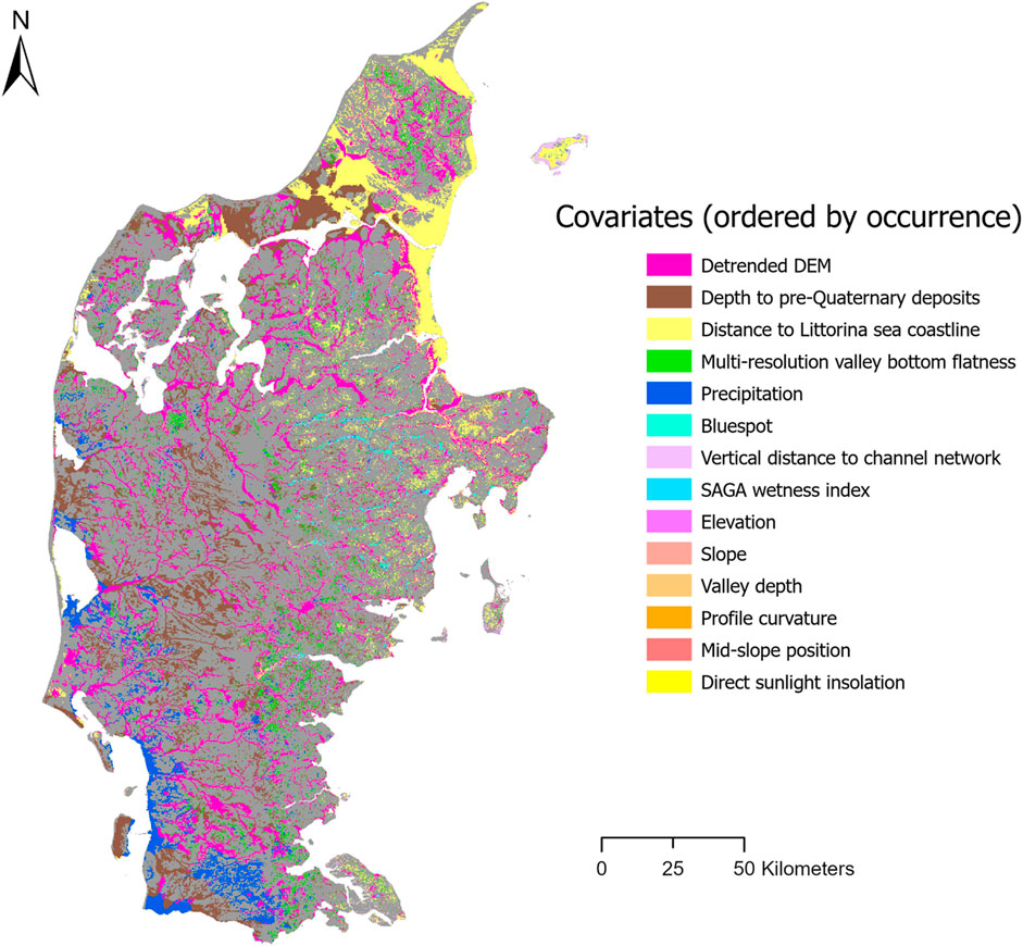
FIGURE 5. Spatial distribution of covariates with the largest SHAP importance for each patch.
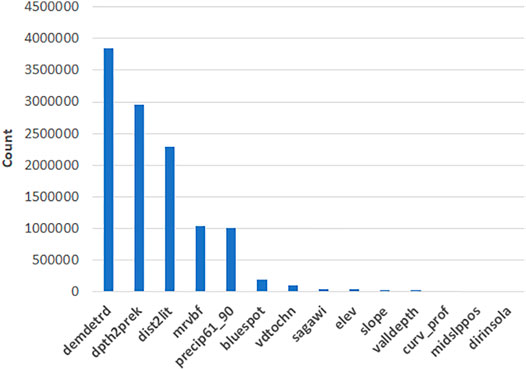
FIGURE 6. Distribution of covariates with the largest SHAP importance for each patch (clarification of covariate names in Table 1).
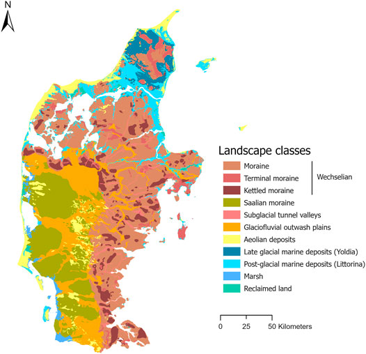
FIGURE 7. Map of the main landscape types (i.e., spatially homogeneous geomorphological units) in Jutland (derived using the existing digital vector landscape map at 1:100000 scale originally from Madsen et al. (1992)).
A summary plot for the selected CNN can be seen in Figure 8. Each point on the plot shows the yielded SHAP values for each covariate for all 5 × 5 patches. It should be noted that if multiple patches for a given covariate have the same value the points are stretched along the y-axis. Notably, the plot confirms the previously developed interpretation results concerning the most important covariates in terms of SHAP contribution and enables further interpretation. Focusing on the detrended DEM, Figure 8 shows that low elevation values (in blue) mostly have a strong positive impact on the model output, which can be explained as soils typically occur in low-lying areas. Shallow depths to pre-Quaternary deposits and small distances to the former Littorina sea coastline (in blue) also present a substantial positive impact on the model output. This confirms that potential AS soils can be targeted in the corresponding areas, either in former marine environments close to the former Littorina sea coastline or in non-marine environments above shallow pyrite-rich Tertiary deposits.
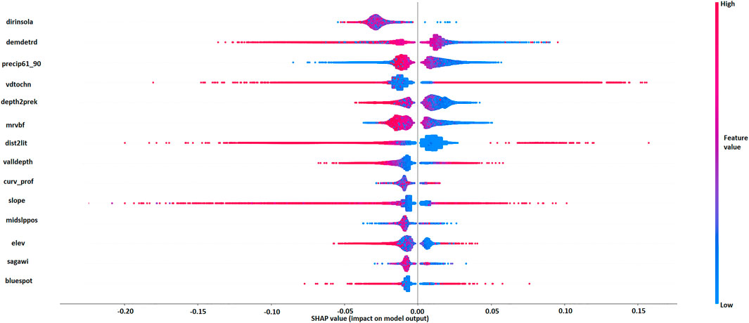
FIGURE 8. Summary plot for the selected CNN model (clarification of covariate/feature names in Table 1).
Next, the distribution of SHAP values for the top three covariates, namely the detrended DEM, depth to pre-Quaternary deposits and distance to Littorina sea coastline, is shown in Figure 9. While Figures 5, 6 display the most important covariates spatially and quantitatively, Figure 9 shows the distribution of SHAP values, both positive and negative, for each of the top three covariates. The three maps confirm previous findings. Firstly, the distance to the former Littorina sea coastline (Figure 9C) presents the most positive SHAP values (i.e. strong positive impact on model output) in northern Jutland and the eastern part of central Jutland, which correspond to post-glacial marine deposit areas (Figure 7). The most negative SHAP values (i.e., negative impact on model output) are mostly located in western and southwestern inland areas of Jutland. Secondly, the depth to pre-Quaternary deposits (Figure 9B) show the most positive SHAP values for areas mostly located in the western half of Jutland, where potential AS soils can form in non-marine environments, such as glacial flood plains and moraine landforms overlaying pyrite-rich Tertiary sediments (Figure 7). The most negative SHAP values are located in coastal areas in northern and southwestern Jutland. Thirdly, the detrended DEM (Figure 9A) presents mostly a positive impact in southern, western and parts of northern Jutland. Negative impact occurs in eastern Jutland and the remaining parts of northern Jutland.
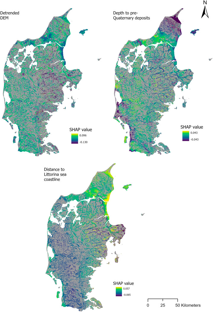
FIGURE 9. Spatial distribution of SHAP values for the three most important covariates: detrended DEM, depth to pre-Quaternary deposits and distance to Littorina sea coastline.
Finally, the Deep SHAP explainer enables assessing covariate importance (as can be done for classical machine learning models such as RF), most importantly in a spatial context, producing different maps of covariate contributions for the CNN predictive model. Concurring with Padarian et al. (2020), we emphasize that the use of SHAP values for model interpretation represents a substantial development within the DSM framework. Samek et al. (2019) states that discovering new patterns within the data through the use of XAI methods such as SHAP (i.e. explaining and interpreting what covariates/features were used for prediction) is often more important than the prediction itself. The results of the present study are consistent with this statement. Furthermore, as the amount of high resolution data will substantially increase in the near future, the use of deep learning models will also most probably expand. Interpretation methods such as SHAP will thus become necessary to 1) improve our understanding of complex model results, 2) possibly develop our knowledge of soil systems and 3) enable us to better explain our findings both to scientific and non-scientific audience.
3.5 Other Challenges Associated With CNNs and Future Possible Development
When employing CNNs, another substantial challenge lies in the selection of a model architecture. Two approaches can be utilized. With the first approach, pre-existing architectures of well-known CNNs such as DenseNet (Huang et al., 2017), Inception (Szegedy et al., 2015), VGG (Simonyan and Zisserman, 2015), Xception (Chollet, 2017) and ResNet (He et al., 2016) are employed. Primarily defined for computer vision, these CNNs have been used for example in land cover classification studies (e.g., Mahdianpari et al. (2018)). With the second approach, a CNN architecture is fully designed and the model trained from scratch. In this case, the network hyperparameters are determined through a highly iterative process which can be based on manual (trial-and-error), purely random or grid search, sequential model-based optimization such as Bayesian optimization or a combination of approaches (Bergstra and Bengio, 2012; Hinz et al., 2018). Within the existing DSM studies investigating the use of CNNS, this second approach is employed. However, the selection of the architecture is generally not clarified, with the exception of Taghizadeh-Mehrjardi et al. (2020b) and Wadoux et al. (2019) which both relied on Bayesian optimization. while the present study utilized Bayesian optimization for the selection of several hyperparameters, it still resorted to a trial-and-error process to design the CNN architecture (i.e., number and type of layers), which constitutes a substantial weakness. A future development of the present work would be to test and clarify different existing methods for hyperparameter optimization, such as tree of Parzen estimators, genetic algorithm and sequential model-based algorithm configuration (Hinz et al., 2018) for the specific purpose of soil mapping.
Another crucial challenge consists in the assessment of uncertainty for CNN model predictions. Padarian et al. (2019b) used bootstrapping to derive confidence intervals while Wadoux (2019) employed a method based on bootstrap plus variance estimates (Khosravi et al., 2011). The latter study also referred to two other possible methods for uncertainty quantification of neural networks, namely the Bayesian uncertainty analysis (Mackay, 1992; Gal and Ghahramani, 2016) and the Delta (De Vleaux et al., 1998) methods, which have not been tested yet. Considering AS soils, the use of contextual information may considerably benefit the mapping of their occurrence. A future development of the present study would be the prediction of key soil properties in strategic hot spot areas for AS soil occurrence using CNNs. Accounting for the spatial variability of soil properties, such as incubation pH and titratable acidity, would enable an improved management of environmental risks related to AS soils.
4 Conclusion
The present study aimed at investigating first, the use of convolutional neural networks for the classification of potential acid sulfate soils located in the wetlands of Jutland, Denmark, and second and most importantly, the application of a model-agnostic interpretation method called SHAP to the selected convolutional neural networks model. The deep learning model yielded slightly higher prediction accuracy than the random forest models which were using original or scaled covariates. These results could most likely be explained by the use of a common variable selection method, namely recursive feature elimination. This technique being based on the random forest algorithm most probably rendered a selection of covariates optimized for this method. However, the main focus of the study was to assess the SHAP interpretation method. In particular, the spatial interpretation of the most important covariates enabled to clarify the predictions of the selected convolutional neural networks model. While classical machine learning methods such as random forest or cubist provide variable importance or usage, SHAP allows the visualization of covariate contribution to the convolutional neural network model at different levels in geographical space, such as the general spatial distribution of all most important covariates in one map and the specific spatial distribution of SHAP values for one covariate. The possibility to inspect the contribution of covariates in space constitutes a crucial development for digital soil mapping in general and for contextual mapping in particular. The combination of convolutional neural networks and SHAP represent a powerful and promising progress for contextual mapping. Furthermore, the rapid developments within the field of explainable artificial intelligence will most likely deliver novel tools to visualize, explain and interpret deep learning methods, which may lead to discovering new insights, improving both knowledge and understanding of soil systems.
Data Availability Statement
The raw data supporting the conclusion of this article will be made available by the authors, without undue reservation.
Author Contributions
AB conceived, executed the research and wrote the paper. CR participated in executing the research and writing the paper. TM reviewed the paper. MG gave suggestions about the approach and reviewed the paper.
Funding
The study was supported by the ReDoCO2 project with funding from the Innovation Fund Denmark (grant number: 0177-00086A).
Conflict of Interest
The authors declare that the research was conducted in the absence of any commercial or financial relationships that could be construed as a potential conflict of interest.
Publisher’s Note
All claims expressed in this article are solely those of the authors and do not necessarily represent those of their affiliated organizations, or those of the publisher, the editors, and the reviewers. Any product that may be evaluated in this article, or claim that may be made by its manufacturer, is not guaranteed or endorsed by the publisher.
References
Abadi, M., Barham, P., Chen, J., Chen, Z., Davis, A., Dean, J., et al. (2016). “Tensorflow: a System for Large-Scale Machine Learning,” in OSDI, 265–283.
Adhikari, K., Hartemink, A. E., Minasny, B., Bou Kheir, R., Greve, M. B., and Greve, M. H. (2014). Digital Mapping of Soil Organic Carbon Contents and Stocks in Denmark. PLoS ONE 9. doi:10.1371/journal.pone.0105519
Batty, M., and Torrens, P. M. (2001). Modelling Complexity : The Limits to Prediction. cybergeo 201. doi:10.4000/cybergeo.1035
Behrens, T., Schmidt, K., Zhu, A. X., and Scholten, T. (2010a). The ConMap Approach for Terrain-Based Digital Soil Mapping. Eur. J. Soil Sci. 61, 133–143. doi:10.1111/j.1365-2389.2009.01205.x
Behrens, T., Zhu, A.-X., Schmidt, K., and Scholten, T. (2010b). Multi-scale Digital Terrain Analysis and Feature Selection for Digital Soil Mapping. Geoderma 155, 175–185. doi:10.1016/j.geoderma.2009.07.010
Behrens, T., Schmidt, K., Ramirez-Lopez, L., Gallant, J., Zhu, A. X., and Scholten, T. (2014). Hyper-Scale Digital Soil Mapping and Soil Formation Analysis. Geoderma 213, 578–588. doi:10.1016/j.geoderma.2013.07.031
Behrens, T., Schmidt, K., MacMillan, R. A., and Viscarra Rossel, R. A. (2018a). Multi-scale Digital Soil Mapping with Deep Learning. Sci. Rep. 8, 2–10. doi:10.1038/s41598-018-33516-6
Behrens, T., Schmidt, K., MacMillan, R. A., and Viscarra Rossel, R. A. (2018b). Multiscale Contextual Spatial Modelling with the Gaussian Scale Space. Geoderma 310, 128–137. doi:10.1016/j.geoderma.2017.09.015
Bergstra, J., and Bengio, Y. (2012). Random Search for Hyper-Parameter Optimization. J. Machine Learn. Res. 13, 281–305.
Beucher, A., Österholm, P., Martinkauppi, A., Edén, P., and Fröjdö, S. (2013). Artificial Neural Network for Acid Sulfate Soil Mapping: Application to the Sirppujoki River Catchment Area, South-Western Finland. J. Geochem. Explor. 125, 46–55. doi:10.1016/j.gexplo.2012.11.002
Beucher, A., Fröjdö, S., Österholm, P., Martinkauppi, A., and Edén, P. (2014). Fuzzy Logic for Acid Sulfate Soil Mapping: Application to the Southern Part of the Finnish Coastal Areas. Geoderma 226-227, 21–30. doi:10.1016/j.geoderma.2014.03.004
Beucher, A., Siemssen, R., Fröjdö, S., Österholm, P., Martinkauppi, A., and Edén, P. (2015). Artificial Neural Network for Mapping and Characterization of Acid Sulfate Soils: Application to Sirppujoki River Catchment, Southwestern Finland. Geoderma, 247-248, 38–50. doi:10.1016/j.geoderma.2014.11.031
Beucher, A., Adhikari, K., Breuning-Madsen, H., Greve, M. B., Österholm, P., Fröjdö, S., et al. (2017). Mapping Potential Acid Sulfate Soils in Denmark Using Legacy Data and LiDAR-Based Derivatives. Geoderma 308, 363–372. doi:10.1016/j.geoderma.2016.06.001
Binzer, K., and Stockmarr, J. (1994). Geological Map of Denmark 1:500,000 – Pre-Quaternary Surface Topography of Denmark. Geological Survey of Denmark. Map series no. 44, 10. 2 maps.
Böhner, J., and Antonić, O. (2009). “Chapter 8 Land-Surface Parameters Specific to Topo-Climatology,” in Geomorphometry: Concepts, Software, Applications. Editors T. Hengl, and H. I. Reuter (New York: Elsevier), 195–226. doi:10.1016/s0166-2481(08)00008-1
Böhner, J., Köthe, R., Conrad, O., Gross, J., Ringeler, A., and Selige, T. (2002). “Soil Regionalization by Means of Terrain Analysis and Process Parameterization,” in Soil Classification 2001. Editors E. Micheli, F. Nachtergaele, and L. Montanarella (Luxembourg), Eur. Soil Bur., Res. Rep. No. 7, EUR 20398 EN 213–222.
Bou Kheir, R., Greve, M. H., Bøcher, P. K., Greve, M. B., Larsen, R., and McCloy, K. (2010). Predictive Mapping of Soil Organic Carbon in Wet Cultivated Lands Using Classification-Tree Based Models: The Case Study of Denmark. J. Environ. Manage. 91, 1150–1160. doi:10.1016/j.jenvman.2010.01.001
Boyle, R., and Thomas, R. (1988). Computer Vision: A First Course. UK: Blackwell Scientific Publications, 210–34.
Brungard, C. W., Boettinger, J. L., Duniway, M. C., Wills, S. A., and Edwards, T. C. (2015). Machine Learning for Predicting Soil Classes in Three Semi-arid Landscapes. Geoderma 239-240, 68–83. doi:10.1016/j.geoderma.2014.09.019
Breuning Madsen, H., and Henrik Jensen, N. (1988). Potentially Acid Sulfate Soils in Relation to Landforms and Geology. Catena 15, 137–145. doi:10.1016/0341-8162(88)90025-2
Cai, J., Luo, J., Wang, S., and Yang, S. (2018). Feature Selection in Machine Learning: A New Perspective. Neurocomputing 300, 70–79. doi:10.1016/j.neucom.2017.11.077
Chagas, C. d. S., Antônio, C., Vieira, O., Elpídio, I., and Fernandes, F. (2013). Comparison Between Artificial Neural Networks and Maximum Likelihood Classification in Digital Soil Mapping. R. Bras. Ci. Solo 37, 339–351.
Chollet, F. (2017). “Xception: Deep Learning with Depthwise Separable Convolutions,” in Proceedings - 30th IEEE Conference on Computer Vision and Pattern Recognition, Honolulu, HI, 2017-January, 1800–1807. CVPR 2017. doi:10.1109/CVPR.2017.195
Conrad, O., Bechtel, B., Bock, M., Dietrich, H., Fischer, E., Gerlitz, L., et al. (2015). System for Automated Geoscientific Analyses (SAGA) V. 2.1.4. Geosci. Model. Dev. 8, 1991–2007. doi:10.5194/gmd-8-1991-2015
Danmarks Meteorologiske Institut (1998). Danmarks Klima 1997. Copenhagen: Danmarks Meteorologiske Institut.
De Vleaux, R. D., Schumi, J., Schweinsberg, J., and Ungar, L. H. (1998). Prediction Intervals for Neural Networks via Nonlinear Regression. Technometrics 40, 273–282. doi:10.1080/00401706.1998.10485556
Emadi, M., Taghizadeh-Mehrjardi, R., Cherati, A., Danesh, M., Mosavi, A., and Scholten, T. (2020). Predicting and Mapping of Soil Organic Carbon Using Machine Learning Algorithms in Northern Iran. Remote Sens. 12, 2234. doi:10.3390/rs12142234
ESRI (2020). ArcGIS Desktop: Release 10.7.1. Redlands, CA: Environmental Systems Research Institute.
Gal, Y., and Ghahramani, Z. (2016). “Dropout as a Bayesian Approximation: Representing Model Uncertainty in Deep Learning,” in 33rd International Conference on Machine Learning, ICML 2016, 1651–1660.
Gallant, J., and Dowling, T. (2003). A Multi-Resolution index of valley Bottom Flatness for Mapping Depositional Areas. Water Resour. Res. 39 (12), 1347–1359. doi:10.1029/2002wr001426
Gershenfeld, N. (1999). The Nature of Mathematical Modelling. Cambridge: Cambridge University Press, 356.
Gholizadeh, A., Saberioon, M., Ben-Dor, E., Viscarra Rossel, R. A., and Borůvka, L. (2020). Modelling Potentially Toxic Elements in forest Soils with Vis-NIR Spectra and Learning Algorithms. Environ. Pollut. 267, 115574. doi:10.1016/j.envpol.2020.115574
Greve, M. H., Christensen, O. F., Greve, M. B., and Kheir, R. B. (2014). Change in Peat Coverage in Danish Cultivated Soils during the Past 35 Years. Soil Sci. 179, 250–257. doi:10.1097/SS.0000000000000066
Grinand, C., Arrouays, D., Laroche, B., and Martin, M. P. (2008). Extrapolating Regional Soil Landscapes from an Existing Soil Map: Sampling Intensity, Validation Procedures, and Integration of Spatial Context. Geoderma 143, 180–190. doi:10.1016/j.geoderma.2007.11.004
Haghi, R. K., Pérez-Fernández, E., and Robertson, A. H. J. (2021). Prediction of Various Soil Properties for a National Spatial Dataset of Scottish Soils Based on Four Different Chemometric Approaches: A Comparison of Near Infrared and Mid-infrared Spectroscopy. Geoderma 396, 115071. doi:10.1016/j.geoderma.2021.115071
He, K., Zhang, X., Ren, S., and Sun, J. (2016). “Deep Residual Learning for Image Recognition,” in Proceedings of the IEEE Computer Society Conference on Computer Vision and Pattern Recognition, 2016-December, 770–778. doi:10.1109/cvpr.2016.90
Hengl, T., Nussbaum, M., Wright, M. N., Heuvelink, G. B. M., and Gräler, B. (2018). Random forest as a Generic Framework for Predictive Modeling of Spatial and Spatio-Temporal Variables. PeerJ 6, e5518. doi:10.7717/peerj.5518
Hijmans, R. (2021). Raster: Geographic Data Analysis and Modeling. r package version 3. 4-13. Available at https://cran.r-project.org/web/packages/raster/.
Hinz, T., Navarro-Guerrero, N., Magg, S., and Wermter, S. (2018). Speeding up the Hyperparameter Optimization of Deep Convolutional Neural Networks. Int. J. Comp. Intel. Appl. 17, 1850008–1850015. doi:10.1142/S1469026818500086
Huang, J., Nhan, T., Wong, V. N. L., Johnston, S. G., Lark, R. M., and Triantafilis, J. (2014a). Digital Soil Mapping of a Coastal Acid Sulfate Soil Landscape. Soil Res. 52, 327–339. doi:10.1071/SR13314
Huang, J., Wong, V. N. L., and Triantafilis, J. (2014b). Mapping Soil Salinity and pH across an Estuarine and Alluvial plain Using Electromagnetic and Digital Elevation Model Data. Soil Use Manage 30, 394–402. doi:10.1111/sum.12122
Huang, G., Liu, Z., Van Der Maaten, L., and Weinberger, K. Q. (2017). “Densely Connected Convolutional Networks,” ,in Proceedings - 30th IEEE Conference on Computer Vision and Pattern Recognition, Honolulu, HI, 2017-January, 2261–2269. CVPR 2017. doi:10.1109/CVPR.2017.243
IUSS Working Group WRB (2006). World Reference Base for Soil Resources 2006. World Soil Resources Reports No. 103. Rome: FAO.
Jiang, Z.-d., Owens, P. R., Zhang, C.-l., Brye, K. R., Weindorf, D. C., Adhikari, K., et al. (2021). Towards a Dynamic Soil Survey: Identifying and Delineating Soil Horizons In-Situ Using Deep Learning. Geoderma 401, 115341. doi:10.1016/j.geoderma.2021.115341
Keras (2021). Available at https://keras.io/.
Khaledian, Y., and Miller, B. A. (2020). Selecting Appropriate Machine Learning Methods for Digital Soil Mapping. Appl. Math. Model. 81, 401–418. doi:10.1016/j.apm.2019.12.016
Khosravi, A., Nahavandi, S., Creighton, D., and Atiya, A. F. (2011). Comprehensive Review of Neural Network-Based Prediction Intervals and New Advances. IEEE Trans. Neural Netw. 22, 1341–1356. doi:10.1109/TNN.2011.2162110
Krizhevsky, A., Sutskever, I., and Hinton, G. E. (2012). “Imagenet Classification with Deep Convolutional Neural Networks,” in Advances in Neural Information Processing Systems (MIT Press), 1097–1105.
Kuhn, M. (2021). Caret: Classification and Regression Training. r package version 6.0-88. Available at https://cran.r-project.org/web/packages/caret/.
Lark, R. M., and Webster, R. (2001). Changes in Variance and Correlation of Soil Properties with Scale and Location: Analysis Using an Adapted Maximal Overlap Discrete Wavelet Transform. Eur. J. Soil Sci. 52, 547–562. doi:10.1046/j.1365-2389.2001.00420.x
Lundberg, S. M., and Lee, S. I. (2017). “A Unified Approach to Interpreting Model Predictions,” in Advances in Neural Information Processing Systems, Long Beach, CA, 2017-Decem, 4766–4775.
Mackay, D. J. C. (1992). The Evidence Framework Applied to Classification Networks. Neural Comput. 4, 720–736. doi:10.1162/neco.1992.4.5.720
Madsen, H. B., Jensen, N. H., Jakobsen, B. H., and Platou, S. W. (1985). A Method for Identification and Mapping Potentially Acid Sulfate Soils in Jutland, Denmark. Catena 12, 363–371. doi:10.1016/s0341-8162(85)80031-x
Madsen, H., Nørr, A., and Holst, K. (1992). “The Danish Soil Classification,” in Atlas over Denmark I (Copenhagen: The Royal Danish Geographical Society), Vol. 3.
Mahdianpari, M., Salehi, B., Rezaee, M., Mohammadimanesh, F., and Zhang, Y. (2018). Very Deep Convolutional Neural Networks for Complex Land Cover Mapping Using Multispectral Remote Sensing Imagery. Remote Sens. 10, 1119. doi:10.3390/rs10071119
Miller, B. A., Koszinski, S., Wehrhan, M., and Sommer, M. (2015). Impact of Multi-Scale Predictor Selection for Modeling Soil Properties. Geoderma 239-240, 97–106. doi:10.1016/j.geoderma.2014.09.018
Molnar, C. (2021). Interpretable Machine Learning - A Guide for Making Black Box Models Explainable. Available at https://christophm.github.io/interpretable-ml-book/.
Ng, W., Minasny, B., Mendes, W. d. S., and Demattê, J. A. M. (2019a). Estimation of Effective Calibration Sample Size Using Visible Near Infrared Spectroscopy: Deep Learning vs Machine Learning. SOIL Discuss., 1–21. doi:10.5194/soil-2019-48
Ng, W., Minasny, B., Montazerolghaem, M., Padarian, J., Ferguson, R., Bailey, S., et al. (2019b). Convolutional Neural Network for Simultaneous Prediction of Several Soil Properties Using Visible/near-Infrared, Mid-infrared, and Their Combined Spectra. Geoderma 352, 251–267. doi:10.1016/j.geoderma.2019.06.016
Padarian, J., Minasny, B., and McBratney, A. B. (2019a). Transfer Learning to Localise a continental Soil Vis-NIR Calibration Model. Geoderma 340, 279–288. doi:10.1016/j.geoderma.2019.01.009
Padarian, J., Minasny, B., and McBratney, A. B. (2019b). Using Deep Learning for Digital Soil Mapping. Soil 5, 79–89. doi:10.5194/soil-5-79-2019
Padarian, J., Minasny, B., and McBratney, A. B. (2019c). Using Deep Learning to Predict Soil Properties from Regional Spectral Data. Geoderma Reg. 16, e00198. doi:10.1016/j.geodrs.2018.e00198
Padarian, J., McBratney, A. B., and Minasny, B. (2020). Game Theory Interpretation of Digital Soil Mapping Convolutional Neural Networks. SOIL Discuss., 1–12. doi:10.5194/soil-2020-17
Porwal, A., Carranza, E. J. M., and Hale, M. (2003). Knowledge-Driven and Data-Driven Fuzzy Models for Predictive Mineral Potential Mapping. Natural Resources Research 12.
Pyo, J., Hong, S. M., Kwon, Y. S., Kim, M. S., and Cho, K. H. (2020). Estimation of Heavy Metals Using Deep Neural Network with Visible and Infrared Spectroscopy of Soil. Sci. Total Environ. 741, 140162. doi:10.1016/j.scitotenv.2020.140162
Python Software Foundation (2021). Python Language Reference, Python Software Foundation. Available at https://www.python.org/.
R Core Team (2021). R: A Language and Environment for Statistical Computing. Vienna Austria: R Foundation for Statistical Computing.
Samek, W., Montavon, G., Vedaldi, A., Hansen, L. K., and Muller, K.-R. (2019). Explainable AI: Interpreting, Explaining and Visualizing Deep Learning. doi:10.1007/978-3-030-28954-6
Scharling, M. (2000). Klimagrid - Danmark Normaler 1961-90 Måneds- Og Årsværdier Nedbør 10*10, 20*20 40*40 422 Km Temperatur Og Potentiel Fordampning 20*20 40*40 Km. Danish Meteorological Institute, 1–17. Teknisk Rapport.
Shapiro, R. (1970). Smoothing, Filtering, and Boundary Effects. Rev. Geophys. 8, 359–387. doi:10.1029/rg008i002p00359
Shrikumar, A., Greenside, P., and Kundaje, A. (2017). “Learning Important Features through Propagating Activation Differences,” in 34th International Conference on Machine Learning, ICML 2017, 4844–4866.
Simard, P. Y., Steinkraus, D., and Platt, J. C. (2003). “Best Practices for Convolutional Neural Networks Applied to Visual Document Analysis,” in Proceedings of the Seventh International Conference on Document Analysis and Recognition (ICDAR), 1–6.
Simonyan, K., and Zisserman, A. (2015). “Very Deep Convolutional Networks for Large-Scale Image Recognition,” in 3rd International Conference on Learning Representations, ICLR 2015 - Conference Track Proceedings, 1–14.
Singh, S., and Kasana, S. S. (2019). Estimation of Soil Properties from the EU Spectral Library Using Long Short-Term Memory Networks. Geoderma Reg. 18, e00233. doi:10.1016/j.geodrs.2019.e00233
Smith, M. P., Zhu, A.-X., Burt, J. E., and Stiles, C. (2006). The Effects of DEM Resolution and Neighborhood Size on Digital Soil Survey. Geoderma 137, 58–69. doi:10.1016/j.geoderma.2006.07.002
Song, X., Zhang, G., Liu, F., Li, D., Zhao, Y., and Yang, J. (2016). Modeling Spatio-Temporal Distribution of Soil Moisture by Deep Learning-Based Cellular Automata Model. J. Arid Land 8, 734–748. doi:10.1007/s40333-016-0049-0
Strobl, C., Boulesteix, A.-L., Zeileis, A., and Hothorn, T. (2007). Bias in Random forest Variable Importance Measures: Illustrations, Sources and a Solution. BMC Bioinformatics 8–25. doi:10.1186/1471-2105-8-25
Sun, X.-L., Wang, H.-L., Zhao, Y.-G., Zhang, C., and Zhang, G.-L. (2017). Digital Soil Mapping Based on Wavelet Decomposed Components of Environmental Covariates. Geoderma 303, 118–132. doi:10.1016/j.geoderma.2017.05.017
Szegedy, C., Wei Liu, W., Yangqing Jia, Y., Sermanet, P., Reed, S., Anguelov, D., et al. (2015). “Going Deeper with Convolutions,” in Proceedings of the IEEE Computer Society Conference on Computer Vision and Pattern Recognition, Boston, MA, 07-12-June, 1–9. doi:10.1109/CVPR.2015.7298594
Taghizadeh-Mehrjardi, R., Mahdianpari, M., Mohammadimanesh, F., Behrens, T., Toomanian, N., Scholten, T., et al. (2020a). Multi-task Convolutional Neural Networks Outperformed Random forest for Mapping Soil Particle Size Fractions in central Iran. Geoderma 376, 114552. doi:10.1016/j.geoderma.2020.114552
Taghizadeh-Mehrjardi, R., Schmidt, K., Amirian-Chakan, A., Rentschler, T., Zeraatpisheh, M., Sarmadian, F., et al. (2020b). Improving the Spatial Prediction of Soil Organic Carbon Content in Two Contrasting Climatic Regions by Stacking Machine Learning Models and Rescanning Covariate Space. Remote Sens. 12, 1095. doi:10.3390/rs12071095
Tao, F., Zhou, Z., Huang, Y., Li, Q., Lu, X., Ma, S., et al. (2020). Deep Learning Optimizes Data-Driven Representation of Soil Organic Carbon in Earth System Model over the Conterminous United States. Front. Big Data 3, 1–15. doi:10.3389/fdata.2020.00017
Tsakiridis, N. L., Keramaris, K. D., Theocharis, J. B., and Zalidis, G. C. (2020). Simultaneous Prediction of Soil Properties from VNIR-SWIR Spectra Using a Localized Multi-Channel 1-D Convolutional Neural Network. Geoderma 367, 114208. doi:10.1016/j.geoderma.2020.114208
Wadoux, A. M. J.-C., Padarian, J., and Minasny, B. (2019). Multi-source Data Integration for Soil Mapping Using Deep Learning. Soil 5, 107–119. doi:10.5194/soil-5-107-2019
Wadoux, A. M. J.-C. (2019). Using Deep Learning for Multivariate Mapping of Soil with Quantified Uncertainty. Geoderma 351, 59–70. doi:10.1016/j.geoderma.2019.05.012
Wright, M. N., and Ziegler, A. (2017). Ranger: A Fast Implementation of Random Forests for High Dimensional Data in C++ and R. J. Stat. Soft. 77. doi:10.18637/jss.v077.i01
Xu, Z., Zhao, X., Guo, X., and Guo, J. (2019). Deep Learning Application for Predicting Soil Organic Matter Content by VIS-NIR Spectroscopy. Comput. Intell. Neurosci. 2019, 1–11. doi:10.1155/2019/3563761
Yan, Y. (2021). rBayesianOptimization: Bayesian Optimization of Hyperparameters. R package version 1.2.0. Available at https://cran.r-project.org/web/packages/rBayesianOptimization/.
Yang, J., Wang, X., Wang, R., and Wang, H. (2020). Combination of Convolutional Neural Networks and Recurrent Neural Networks for Predicting Soil Properties Using Vis-NIR Spectroscopy. Geoderma 380, 114616. doi:10.1016/j.geoderma.2020.114616
Keywords: convolutional neural network, XAI (eXplainable artificial intelligence), SHAP (SHapley Additive exPlanations), interpretability, deep learning, classification, acid sulfate soils
Citation: Beucher A, Rasmussen CB, Moeslund TB and Greve MH (2022) Interpretation of Convolutional Neural Networks for Acid Sulfate Soil Classification. Front. Environ. Sci. 9:809995. doi: 10.3389/fenvs.2021.809995
Received: 05 November 2021; Accepted: 09 December 2021;
Published: 19 January 2022.
Edited by:
Ruhollah Taghizadeh-Mehrjardi, University of Tübingen, GermanyCopyright © 2022 Beucher , Rasmussen, Moeslund and Greve . This is an open-access article distributed under the terms of the Creative Commons Attribution License (CC BY). The use, distribution or reproduction in other forums is permitted, provided the original author(s) and the copyright owner(s) are credited and that the original publication in this journal is cited, in accordance with accepted academic practice. No use, distribution or reproduction is permitted which does not comply with these terms.
*Correspondence: Amélie Beucher , YW1lbGllLmJldWNoZXJAYWdyby5hdS5kaw==