Distributed PV carrying capacity prediction and assessment for differentiated scenarios based on CNN-GRU deep learning

The increasing penetration of distributed photovoltaic (PV) brings challenges to the safe and reliable operation of distribution networks, distributed PV access to the grid changes the characteristics of the traditional distribution grid. Therefore, the assessment of distributed PV carrying capacity is of great significance for distribution network planning. To this end, a differentiated scenario-based distributed PV carrying capacity assessment method based on a combination of Convolutional Neural Networks (CNN) and Gated Recurrent Unit (GRU) is proposed. Firstly, the meteorological characteristics affecting PV power are quantitatively analyzed using Pearson’s correlation coefficient, and the influence of external factors on PV power characteristics is assessed by integrating the measured data. Then, for the problem of high blindness of clustering parameters and initial clustering centers in the K-means clustering algorithm, the optimal number of clusters is determined by combining the cluster Density Based Index (DBI) and hierarchical clustering. The improved K-means clustering method reduces the complexity of massive scenarios to obtain distributed PV power under differentiated scenarios. On this basis, a distributed PV power prediction method based on the CNN-GRU model is proposed, which employs the CNN model for feature extraction of high-dimensional data, and then the temporal feature data are optimally trained by the GRU model. Based on the clustering results, the solution efficiency is effectively improved and the accurate prediction of distributed PV power is realized. Finally, taking into account the PV access demand of the distribution network, combined with the power flow calculation of distribution network, the bearing capacity of distribution network considering node voltage in differentiated scenarios is evaluated. In addition, verified by source-grid-load measured data in IEEE 33-bus distribution system. The simulation results show that the proposed CNN-GRU fusion deep learning model can accurately and efficiently assess the distributed PV carrying capacity of the distribution network and provide theoretical guidance for realizing distributed PV access on a large scale.

1 Introduction

In recent years, with the aggravation of fossil energy shortage and environmental pollution issues, new energy is developing rapidly under the promotion of national policies and technological development. As an effective form of new energy utilization, distributed photovoltaic (PV) has the advantages of cleanliness, efficiency, and flexibility (Haghdadi et al., 2018). With the development of clean energy strategies in various countries, distributed power sources represented by wind power, PV, etc. are developing rapidly, and their large-scale access to the distribution network has become an unstoppable trend (Huang et al., 2024).

Distributed PV output is closely related to the local real-time solar irradiation intensity, with obvious intermittency and volatility (Wang et al., 2022). Large-scale distributed PV access to the grid has changed the characteristics of the traditional distribution network. The distribution network is transformed from the passive network to the active network, and the distribution network flow is transformed from unidirectional to bidirectional. It has brought many adverse effects on the voltage (Fernández et al., 2020), power quality (Li et al., 2023), relay protection (Jia et al., 2018), planning (Xiao et al., 2022), and dispatching operation (Cheng et al., 2024) of the distribution network, which seriously threatens the safe and stable operation of the distribution network. In addition, distributed PVs are usually located at the end of the distribution network, with low access voltage levels, poor observability and measurability, and often unpredictable security risks caused by their disorderly access. Therefore, in order to ensure the coordinated development of source-grid-load it is necessary to predict and evaluate the distributed PV power and carrying capacity based on the differentiated scenarios of the distribution network, and then provide guidance for the planning and construction of the distribution network.

In recent years domestic and foreign scholars have conducted extensive research work on PV generation power prediction, mainly focusing on physical methods (Antonanzas et al., 2016), statistical learning methods (Li et al., 2014), and combined methods (Zhang et al., 2024). Among them, the physical method establishes an analytical model of meteorological factors (irradiance, temperature, humidity, etc.) affecting power based on the principle of PV power generation, to directly calculate the PV power prediction value through meteorological forecast data and power model (Dolara et al., 2015). Such methods are not strongly dependent on historical power data, but it is usually difficult to establish an accurate analytical model because the PV conversion process involves complex coupling of multiple links (Juan et al., 2024). Statistical learning methods do not focus on the physical process of photovoltaic conversion and use a data-driven approach to directly predict distributed PV output power by modeling the mapping between input variables and power using historical data samples (Zhang et al., 2022). Common statistical learning methods include time series methods (Succetti et al., 2020; Xie et al., 2024), support vector machines (SVM) (Jang et al., 2016), and neural network algorithms (Chen et al., 2023). Although statistical learning methods greatly simplify the modeling process, they place high demands on the quantity and quality of historical data (Theocharides et al., 2020). The combination approach complements the strengths and weaknesses of multiple prediction models, thereby improving the performance prediction accuracy (Ge et al., 2023). Combination methods can be divided into two types: the first involves selecting two or more statistical prediction methods, and combining their results through weighting to obtain the PV power prediction results (Zhen et al., 2019), and the second is by using sequence decomposition techniques to divide the time series data into multiple signal sequences, and using prediction models to predict and sum each sequence separately, thus generating power is obtained (Wang and Lin, 2023).

Current PV power prediction research is mainly divided into two aspects: data pre-processing and prediction models. Among them, data processing is mainly aimed at preprocessing and analyzing single distributed PV data parameters, and there are relatively few researches involving data clustering and integration of distributed PV differentiated scenarios. In terms of prediction models, some of the fusion prediction models have achieved better results in prediction accuracy than the traditional prediction models. However, the application of power prediction models in existing studies in practical engineering applications is relatively limited, and there are fewer studies on the carrying capacity of distribution networks. Considering the various operation indexes of the distribution network, it is difficult to obtain the current situation of historical data, and dealing with the uncertainty problem also faces many difficulties.

Under the current trend of power system transformation to clean energy, large-scale grid integration of distributed PV brings new challenges to the safe and stable operation of distribution networks. Given the practical issues of volatility and time variation in distributed PV output power, assessing the carrying capacity of distribution networks with uncertainty factors is of great significance. Based on this, the paper proposes a distributed PV carrying capacity prediction and assessment method for differentiated scenes based on CNN-GRU deep learning. Firstly, the influence of external environmental factors on distributed PV output characteristics is systematically analyzed in the context of grid connection. Then, the accuracy of PV power prediction is improved by clustering integration and multi-model fusion to provide theoretical support and data reference for the assessment of distribution network carrying capacity after grid-connection of distributed PV. Finally, the proposed hybrid deep learning model is applied in the IEEE 33-bus distribution system to study the carrying capacity of the distribution network under different PV access states, which verifies the effectiveness of the proposed method for the carrying capacity assessment of the distribution network, and provides a certain reference value for the planning and operation of the distribution network. Compared with the traditional method, the proposed method in the paper contributes as follows:

1. By systematically analyzing the external environmental factors of distributed PV, the PV power prediction model is simplified based on improved K-means and hierarchical clustering scenario generation methods, which further improves the efficiency of carrying capacity calculation.

2. The proposed PV power prediction model, based on clustering integration analysis and deep hybrid learning algorithm, can effectively mitigate the adverse effects of distributed energy on distribution networks and can adapt to the actual operation scenarios of distribution networks.

3. Evaluating the PV carrying capacity under differentiated scenarios provides effective method support for distributed PV grid-connected management.

The remainder of the paper is organized as follows. Section 2 analyzes the influencing factors of distributed PV output power and investigates the coordinated characteristics of source load. Section 3 proposes an improved K-means clustering method to classify the scenarios of distributed PV output scenarios. Based on the previously established clustering method, Section 4 introduces a distributed PV power prediction method based on the CNN-GRU model. Section 5 conducts simulation verification of the proposed clustering method and the prediction model. Finally, Section 6 presents the conclusions.

2 Distributed PV power influencing factors and characterization

2.1 Correlation analysis of factors affecting PV power characteristics

The output power of PV power generation is related to various factors, whether it is the geographical location of the PV power station, environmental factors, and the selection of the power generation components, etc., which all have a certain impact on PV power (Ganti et al., 2022). The structure of the PV power generation is shown in Figure 1.

Figure 1

Figure 1. PV system topology.

PV power is significantly affected by fluctuations in meteorological factors such as wind speed, irradiance, barometric pressure, and temperature, and fluctuations in these parameters directly lead to fluctuations in output power. The expressions for output power and output current for PV power generation are shown in Equation 1.

$\left\{\begin{array}{l}{P}_{\text{PV}}=n_{\mathrm{p}}{V}_{pv}\left(I_{\text{ph}}-I_{\text{sat}}\left(\exp \left(\frac{q}{nkT}\frac{V_{\text{pv}}}{n_{\mathrm{s}}}\right)-1\right)\right)\\ I_{\text{ph}}=\left(I_{\text{cr}}+\frac{K_{\mathrm{c}}}{1000}\left(T-T_{\mathrm{c}}\right)\right)S_{\mathrm{c}}\end{array}\right.(1)$

where P_PV and V_PV respectively represent the output power and output voltage of PV; n_s and n_p respectively represent the number of series and parallel PV arrays; I_sat is the dark saturation current; q denotes electronic charge and its value is 1.6 × 10⁻¹⁹ J/k; I_PV represents the output current of PV; k denotes the Boltzmann constant and its value is 1.38 × 10⁻²³ J/k; k is ideality factor; T and T_c respectively represent absolute temperature and reference temperature; I_cr represents the short-circuit current under the reference temperature and solar irradiance per unit area; k_r is the temperature coefficient of the short-circuit current; S_c is the solar radiation intensity. It can be seen from the equation that PV output power is affected by solar irradiance and temperature.

However, including all meteorological factors that affect PV power generation in the prediction model would increase the complexity of the model. Therefore, The paper uses the Pearson correlation coefficient to analyze the correlation between the parameters and selects the meteorological factors that have a stronger correlation with output power.

The Pearson correlation coefficient is used to describe the linear relationship between two variables in mathematical statistics and is a linear correlation coefficient as shown in Equation 2, Jebli et al. (2021).

$r=\frac{{\displaystyle \sum _{i=1}^n}\left(x_i-\overline{x}\right)\left(y_i-\overline{y}\right)}{\sqrt{{\displaystyle \sum _{i=1}^n}{\left(x_i-\overline{x}\right)}^2{\displaystyle \sum _{i=1}^n}{\left(y_i-\overline{y}\right)}^2}}(2)$

where x represents environmental meteorological factors, such as solar radiation intensity, temperature, relative humidity, wind speed, and rainfall, and n represents the number of data points for calculating each meteorological factor; y represents PV output power; $\overline{x}$ and $\overline{y}$ represent the average values of each variable; r is the correlation coefficient, and the larger its absolute value, the stronger the correlation between variables. The correlation degree of the coefficient is shown in Table 1.

Table 1

Table 1. The specific correlation degree of the coefficient.

The data from a PV power station in Xinjiang Province, China, over 1 month were selected, and the Pearson correlation coefficient was used to obtain the correlation coefficients between various meteorological characteristics and power generation. The calculation results are shown in Figure 2.

Figure 2

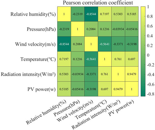
Figure 2. Pearson’s correlation coefficient of PV power generation with each meteorological feature.

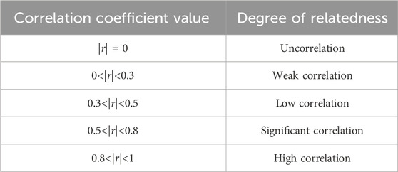
As shown in Figure 2, solar radiation intensity has the highest correlation with PV power generation, with a Pearson correlation coefficient of 0.9479, indicating a high correlation with PV power generation, which is close to complete correlation. Solar irradiance is the most important influencing factor for PV power generation. The Pearson correlation coefficients for temperature and relative humidity are 0.697 and 0.5185, respectively, indicating significant correlation with PV generation power. The Pearson correlation coefficient of wind speed meteorological characteristics is −0.3198, which is a low correlation with PV generation power. Therefore, this paper selects the three features of solar radiation intensity, temperature, and humidity, which are highly correlated with PV power generation, as meteorological input features and combines them with previous PV power generation as the input features of the model. The impact of major meteorological features on PV power generation is analyzed by intercepting PV-specific operating periods.

2.2 Meteorological influences on PV output power

The core of the PV power generation system is the PV cell, which converts solar energy into electricity through the PV effect of semiconductor materials. Therefore, solar irradiance and power generation have a close relationship, and irradiance has a direct influence on determining the output power of a PV power generation system. Solar irradiance and PV power generation are positively correlated (Bucciarelli, 1986). Their physical relationship is shown in Equation 3.

$p=\alpha MS\left[1-0.005\left(t_0-25\right)\right](3)$

where α is conversion efficiency; M represents the area of the PV panel; S is the irradiation intensity; t₀ represents ambient temperature.

From Equation 3, it can be concluded that there is a positively correlated linear relationship between irradiance and PV power. In order to verify this correlation, 5 days of measured data in spring were selected for analysis. Figure 3A shows the joint curve of irradiance and PV power. From the trend graph, it can be seen that as the irradiance increases, the PV output power increases accordingly, and the trend of the two curves is basically the same. Typically, the value of irradiance directly reflects the advantages and disadvantages of meteorological conditions. Therefore, in the prediction of PV power generation, the changes in irradiance must be fully considered.

Figure 3

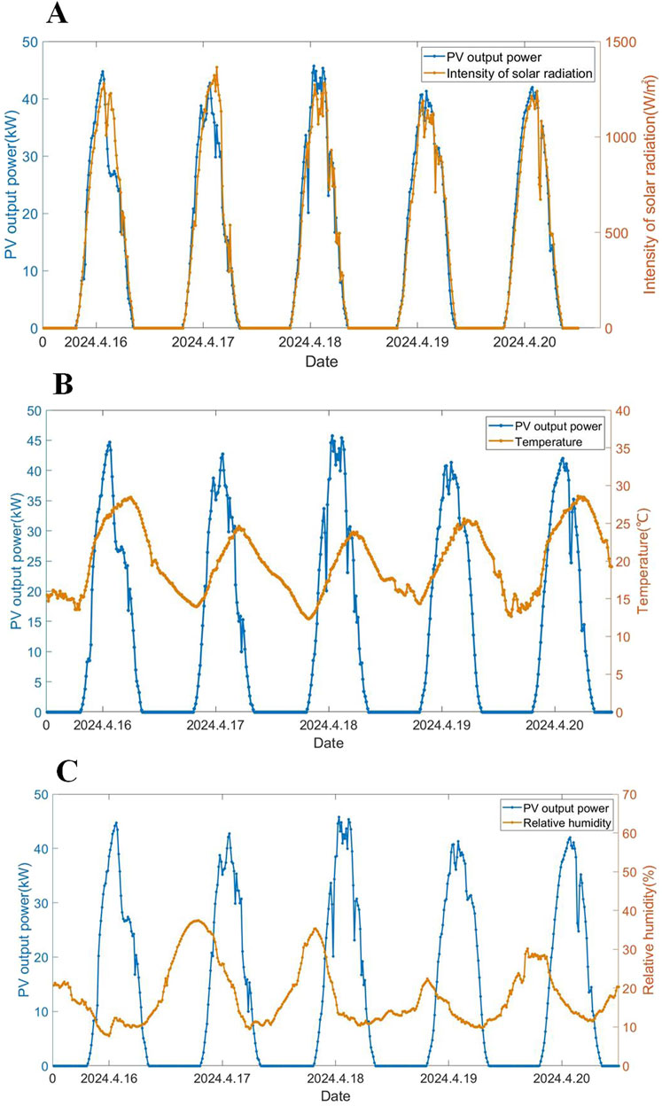
Figure 3. Combined curve diagram of PV power and meteorological factors. (A) Combined PV power and solar irradiance graph. (B) Combined PV power and ambient temperature graph. (C) Combined PV power and relative humidity graph.

A rise in environmental temperature leads to an increase in irradiance and an increase in the operating temperature of the PV cells, which affects the power generation of the PVs. The effect of temperature on PV power is not a simple linear relationship. For example, under extreme weather conditions such as cold winters or hot summers, the performance of solar panels can change significantly, which in turn affects PV output power. Therefore, in the process of PV power prediction, environmental and weather data need to be fully collected to provide accurate data support for high-precision power prediction. To visualize the effect of temperature on PV power, Figure 3B shows the trend of environmental temperature and PV generation power. It can be seen from the figure that the actual output power is approximately positively correlated with the ambient temperature within a certain range. However, the temperature profile is highly volatile, and output efficiency decreases when the solar panel temperature increases to a certain level.

The greater the humidity of the air, the greater the light attenuation phenomenon in the atmosphere, resulting in a corresponding reduction in irradiance. In addition, the higher the relative humidity, the worse the conduction heat dissipation ability of the PV module, leading to a decrease in the system temperature rise efficiency, which indirectly affects the stability and reliability of the PV output power. Based on the data analysis, it is found that when the humidity increases by 1%, the power generation of the power plant may decrease by 0.5%–2%. Figure 3C shows the joint curve of PV output power and humidity. As illustrated in the figure, there is a negative correlation between humidity and photovoltaic power. The minimum value of humidity corresponds to the peak of PV power, and the maximum value of humidity corresponds to the trough of PV power. Since temperature is inversely proportional to humidity, and PV output is positively correlated with temperature, the conversion leads to a certain negative correlation between PV output and relative humidity. When constructing the PV power prediction model, humidity needs to be taken into account as a factor because too high a humidity level may lead to a decrease in irradiance, making PV power generation less efficient.

3 PV differentiated scene clustering method based on improved K-means

The meteorological environment has a significant impact on the power of distributed generation. In order to obtain relatively accurate output power values, a clustering algorithm is used to differentiate between different weather conditions. To reduce the complexity of distributed PV output data processing and analysis, this paper proposes a clustering algorithm to simplify large amounts of PV output data into typical differentiated output scenarios.

3.1 Basic principles of the K-means clustering algorithm

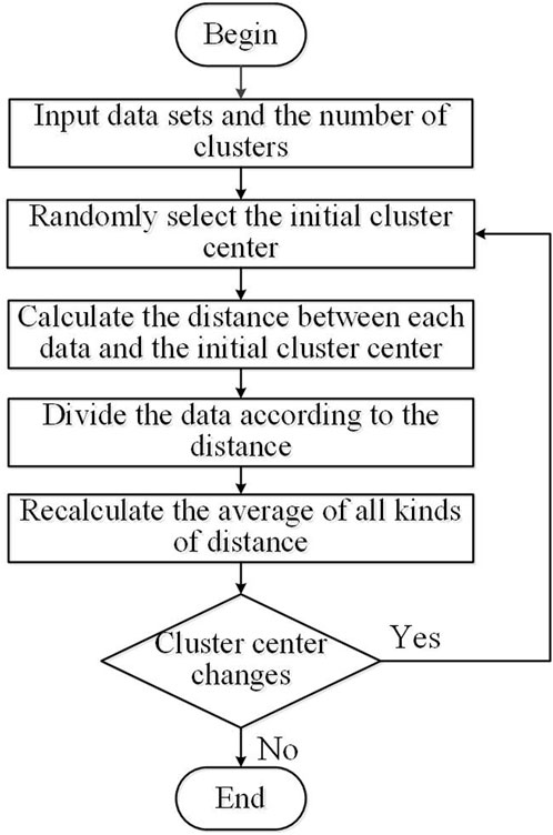
The K-means clustering algorithm classifies data into clusters according to their similarity and uses the distance between samples as a measure of similarity (Kanungo et al., 2002). The basic K-means clustering algorithm process is shown in Figure 4.

Figure 4

Figure 4. Flowchart of basic K-means clustering algorithm.

As shown in the figure, the basic K-means algorithm flow is: First, initialize the dataset and determine the number of clusters, which is the value of k representing the number of typical scenarios to be generated.

3.2 Improved K-means clustering algorithm

The basic K-means clustering algorithm requires the number of clusters to be specified manually, and the cluster centers are randomly generated, both of which can lead to changes in the clustering results. On the one hand, the artificially specified number of clusters cannot reflect typical and extreme PV output conditions; on the other hand, the selection of random cluster centers may fall into a local optimum. Based on the above problems, and to ensure that the differentiated scenarios after clustering are typical, this paper introduces the Density Based Index (DBI) to determine the optimal number of clusters and improves the K-means clustering algorithm by combining it with the hierarchical clustering algorithm.

3.2.1 Determine the optimal number of clusters based on DBI

The DBI index comprehensively considers the dispersion of different clusters and the compactness of the same cluster. The result is mainly expressed by the ratio of the distance between the elements in the cluster and the distance between different clusters. The smaller the value, the greater the difference between the various types, the closer the elements within the same type, and the better the final result. The concept of DBI can be defined as follows (Pan et al., 2022; Li et al., 2019):

First, the intra-cluster dispersion S_i indicator is defined, which represents the average distance from all the scenarios of a certain category to the centroid of the cluster and reflects the dispersion of the time series in the same cluster. The smaller the value, the better the classification effect. The calculation formula is shown in Equation 4:

$S_i=\frac{1}{N_i}{\displaystyle \sum _{j=1}^{N_i}}{\left({\displaystyle \sum _{k=1}^{24}}{\left|X_{ij,k}-A_{i,k}\right|}^2\right)}^{1/2}(4)$

where N_i represents the number of scenes in cluster i; X_ij,k denotes the PV output power at the kth sampling time in the jth scenario of cluster i; A_i,k represents the PV output power of the kth sampling point in the cluster center scenario of cluster i.

The inter-cluster separation M_ij is defined as the Euclidean distance between the cluster center of cluster i and the cluster center of cluster j, which reflects the degree of separation between the various types. The greater the value, the better the classification effect. The calculation formula is shown in Equation 5:

$M_{ij}={‖A_i-A_j‖}_p={\left({\displaystyle \sum _{k=1}^{24}}{\left|A_{i,k}-A_{j,k}\right|}^2\right)}^{1/2}(5)$

where A_i and A_j represent the cluster center scenarios of cluster i and cluster j, respectively; A_i,k and A_j,k represent the output data of the kth sampling point.

The similarity R_ij indicates the ratio of the intra-cluster dispersion to the inter-cluster separation and reflects the degree of similarity between the various types. The smaller the value, the better the classification effect, as shown in Equation 6.

$R_{ij}=\frac{S_i+S_j}{M_{ij}}(6)$

The maximum similarity of cluster i is calculated and denoted as R_i. The formula is shown in Equation 7.

$R_i={\max }_{j\ne i}\left(R_{i1},R_{i2},\dots R_{ij},\dots R_{iK}\right)(7)$

The worst result between cluster i and the other clusters is taken out, and the mean value is calculated to obtain the DBI index, which is expressed as Equation 8:

$DBI=\overline{R}=\frac{1}{K}{\displaystyle \sum _{i=1}^K}{R}_i(8)$

where K represents the number of classifications. Different numbers of categories will produce different DBI values. The smaller the value, the less dispersed the categories, the greater the dispersion between categories, and the better the classification effect.

Finally, set a range of cluster numbers and perform multiple clustering on the same sample, respectively calculating the DBI index. The cluster number corresponding to the minimum value is the optimal value.

3.2.2 Select cluster centers in combination with hierarchical clustering

The basic idea of hierarchical clustering is to group data by calculating the similarity between data points (Fu et al., 2019). Hierarchical clustering starts with a single data point and combines the two most similar data points each time, repeating until the entire data set is combined into a cluster. To improve the K-means clustering algorithm, hierarchical clustering is combined as follows: First, the distance between the scenes is calculated according to the ward variance minimization method to determine the similarity of each scene. Then, all initial cluster centers are determined in order of decreasing overall similarity. The Ward variance minimization method minimizes the increase in the sum of the squares of the distances of the data points in the cluster to their respective means by adjusting the cluster division. The distances of the merged sub-clusters calculated using this method are shown in Equation 9:

$d\left(x_i,x_j\right)=\sqrt{\frac{n_i{n}_j}{n_i+n_j}}{‖{\mu }_i-{\mu }_j‖}_2(9)$

where n_i and n_j are the number of data points in each subcluster, respectively; μ_i and μ_j represent the average value of each sub-cluster feature vector; ||·||₂ denotes the Euclidean distance.

3.3 Differentiated scene generation based on improved K-means clustering algorithm

In summary, the process of generating differentiated scenarios for distributed PV power generation based on the improved K-means clustering algorithm is shown in Figure 5.

Figure 5

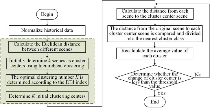
Figure 5. Flowchart of the differentiated scene generation process based on the improved K-means clustering algorithm.

As shown in the figure, the typical scenario generation steps for distributed PV differentiation are as follows.

1. Obtain the original PV scenario time series data.

2. Normalize the original PV scenario data, which is expressed as Equation 10:

$D_i=\frac{D_i}{\max \left(D_1,D_2,\cdots ,D_n\right)-\min \left(D_1,D_2,\cdots ,D_n\right)}(10)$

where D_i represents the ith original data of PV; n denotes the number of original scenes; max (S₁, S₂, … S_n) and min (S₁, S₂, … S_n) represent the maximum and minimum values in the PV raw data within the scene range, respectively.

3. According to the hierarchical clustering approach, select the initial cluster centers and initially determine k typical scenarios.

4. Determine the optimal number of clusters K based on the DBI index. The k corresponding to the minimum DBI value is the optimal number of typical scenarios K.

5. Calculate the distance from all scenarios D in the original scenario to each initial cluster center A. This is expressed as Equation 11:

$O\left(m,q\right)=\sqrt{{\left(D_{m,1}-A_{q,1}\right)}^2+{\left(D_{m,2}-A_{q,2}\right)}^2+\cdots +{\left(D_{m,n}-A_{q,n}\right)}^2}(11)$

where O (m,q) represents the Euclidean distance from the mth scene in the original scene set D to the qt initial clustering center. D_m,n represents the output data of the nth sampling point in the mth scenario; A_q,n represents the output data of the nth sampling point corresponding to the qt cluster center.

6. Evaluate the distance between the mth original scene and each cluster center, and assign it to the cluster with the shortest distance to form the cluster $X=\left\{X_1,X_2,\dots ,X_k\right\}$. The number of scenes in each cluster is calculated and denoted as $T_1,T_2,\dots ,T_k$.

7. Recalculate the clustering center in each cluster, where the center in the tth cluster is expressed as Equation 12:

$A_t=\frac{X_t^1+X_t^2+\cdots +X_t^{T_t}}{T_t}(12)$

where A_t represents the tth new cluster center; $X_t^1$ represents the first group of PV power data in the t cluster; T_t represents the number of scenes in the tth cluster.

8. Determine whether the distance between the cluster centers before and after the update is less than the threshold. If it is greater than the set threshold, return to step 5 and continue the iteration. If it is less than the set threshold, the iteration stops. The final clustering result describes the typical difference in the distributed PV scenario.

4 PV power prediction model based on CNN-GRU deep learning

4.1 CNN algorithm principle

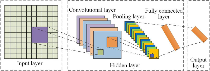
The CNN algorithm belongs to the feedforward neural network, which is usually composed of a convolution layer, pooling layer, and fully connected layer. It can extract the high-level features of the input data layer by layer and finally output the classification or regression results of the data. The commonly used internal structure of CNN is shown in Figure 6.

Figure 6

Figure 6. Structure diagram of CNN.

As shown in the figure, the CNN structure is:

1. Input layer: The input layer is mainly used to pre-process the data or images input into the model to reduce the impact of data volume differences on the model analysis results, making the model more efficient.

2. Hidden layer: The hidden layer can be divided into three layers: pooling layer, convolutional layer, and fully connected layer, which are responsible for extracting features and completing related learning tasks.

a) Convolutional layer: The convolutional kernel in the convolutional layer is the most critical part, responsible for processing the image or data. When training the model, the step size and the number and size of the convolutional kernels can be adjusted based on actual needs.

b) Pooling layer: The pooling layer is mainly responsible for reducing the dimensionality of the sampled data, that is, reducing the dimensionality of the data as much as possible without affecting the characteristics of the data or image. The pooling function can be used to replace a point in the feature map with the global features of the adjacent output.

c) Fully connected layer: The fully connected layer effectively connects the weights of neurons and passes the corresponding information to the next layer of the network. This means the weighted sum of the feature vectors is calculated and processed using matrix multiplication, and then the output of the layer is obtained using an activation function, as shown in Equations 13, 14.

${\mathrm{x}}^l=f\left({\mathrm{u}}^l\right)(13)$

${\mathrm{u}}^l={\mathrm{W}}^l{\mathrm{x}}^{l-1}+{\mathrm{b}}^l(14)$

where x^l-1 represents the input, and by calculating the weighted bias of x^l-1, the activation function of the fully connected layer can be obtained. The weight coefficients w^l and b^l are biased, and then the output of the fully connected layer can be obtained based on the activation function f.

3. Output layer: In this layer, the output values obtained from the fully connected layer are input to obtain the nonlinear transformation result of the nonlinear mapping of the neural network.

4.2 GRU algorithm principle

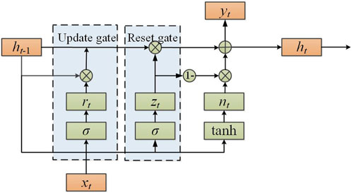
GRU is a variant of Long Short-Term Memory (LSTM). GRU is more efficient in terms of computational time, uses fewer parameters, and has lower complexity, which speeds up network training and convergence (Xie et al., 2022). GRU completes recursive processing through the introduction of time series direction; each node is chain-connected, and it has a memory function in the network. It is currently widely used in many fields such as prediction, classification, and recognition. Its internal structure is shown in Figure 7.

Figure 7

Figure 7. Structure diagram of GRU.

GRU has a self-recurrent gated structure similar to LSTM, which is effective in solving the problem of gradient disappearance. GRU uses an update gate and a reset gate to control the update of the state vector h_t. The update and reset gates of GRU are the key to the training process. The feature quantity involved in training the model includes the state vector h_t-1 of the previous moment; the current input x_t; the current time state vector h_t; the update gate state vector r_t; the current moment candidate state vector h_t^’; and the reset gate state vector z_t. The detailed training process is as follows:

1. First, obtain z_t and r_t. After inputting x_t in the model, it is concatenated with h_t-1 to complete the matrix splicing, and then calculated with the parameter matrices w_r and w_z respectively to obtain z_t and r_t. The detailed algorithm flow is shown in Equations 15, 16.

${\mathrm{z}}_t=\sigma \left({\mathrm{w}}_z\left[h_{t-1},x_t\right]\right)(15)$

${\mathbf{r}}_t=\sigma \left({\mathbf{w}}_r\left[h_{t-1},x_t\right]\right)(16)$

where σ represents the sigmoid function, which can map the input data to a value in the (0, 1) interval, then treat the value as a gated signal.

2. Obtain the current moment candidate state vector h_t^’, as shown in Equation 17.

${\mathbf{h}}_t^{\prime }=\tanh \left(w_h\cdot \left[r_t\times h_{t-1},x_t\right]\right)(17)$

where w_h represents the parameter matrix to be learned; tanh is a hyperbolic tangent function, which can convert the input data into values in the (−1, 1) interval.

3. Update the formula and complete the two functions of “memory” and “forgetting,” as shown in Equation 18.

${\mathbf{h}}_t=\left(1-z_t\right)\times h_{t-1}+z_t\times h_t^{\prime }(18)$

4. Output phase: Learn various parameters and train the model with the aforementioned content, then output the result y_t, as shown in Equation 19.

${\mathbf{y}}_t=\sigma \left(w_t\cdot h_t\right)(19)$

4.3 The structure of the PV carrying capacity assessment model based on CNN-GRU

The GRU algorithm has high accuracy and efficiency in power prediction, but it requires human determination of feature relationships and cannot uncover the correlation of discontinuous features in high-dimensional space. CNN has advantages in the field of data mining, therefore a PV power prediction method based on CNN-GRU is constructed.

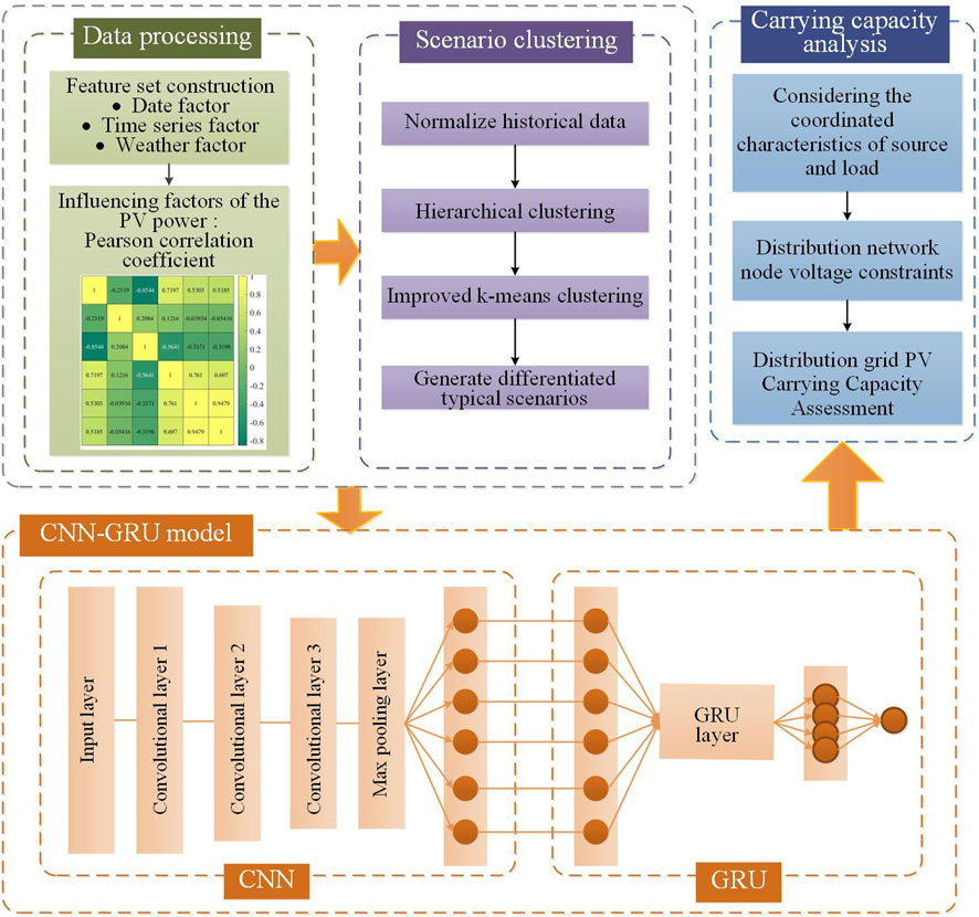
When predicting by this method, the prediction model first clusters and integrates the PV power data and then inputs it to the input layer. Next, the convolutional layer and max pooling layer in the CNN are used to extract features from the time series data and construct a feature vector for the time series data. Among them, CNN consists of multiple convolutional layers that perform multiple convolution operations to capture meaningful information. Finally, the expanded time-series feature vector is used as the input to the GRU to complete the modeling and processing of the sequence data. This method can improve the depth and breadth of the features extracted by the neural network, making the prediction results more accurate.

A large number of distributed PVs connected to the grid will have a great impact on the safe operation of the distribution network, and the unreasonable access of PVs will lead to problems such as overloading of the lines and voltage overruns at some nodes. Therefore, a distribution network carrying capacity assessment method based on the PV power prediction model is constructed. Distribution network PV carrying capacity generally refers to the maximum capacity of PV that can be accessed under the conditions of ensuring the safety, reliability and voltage quality of the distribution network (Wang, 2020). The access of distributed PV has a lifting effect on the voltage of each node, and the more PVs are accessed, the higher the voltage is lifted, and a voltage deviation limit value needs to be set to ensure the safe and stable operation of the power grid. If the value is set low, it will limit the access of distributed PV. If the value is set too high, it will threaten the safe operation of the power system. The corresponding nodal voltage constraint equation is shown in Equation 20:

$U_{\mathrm{N}}\left(1-{\epsilon }_1\right)\le U_i\le U_{\mathrm{N}}\left(1+{\epsilon }_2\right)(20)$

where U_N represents the rated voltage of the distribution network; U_i represents the voltage magnitude at node i; ε₁ and ε₂ are the allowable voltage deviation rates specified in the national standard.

Based on the distributed PV power prediction model constructed above, the PV predicted power is used as an input parameter. Using the distribution network trend calculation method, the distribution network node voltage is calculated after the distributed PV is connected to the grid, to realize the assessment of the distributed PV carrying capacity. The structure diagram of distributed PV carrying capacity prediction and evaluation based on CNN-GRU is shown in Figure 8.

Figure 8

Figure 8. Structure diagram of distributed PV carrying capacity assessment based on CNN-GRU.

5 Case analysis

5.1 Differentiated analysis of typical scenario characteristics

To verify the effectiveness of the proposed clustering algorithm, the PV power generation data and meteorological data of a region in Xinjiang Province, China, in 2023 were selected as the dataset. The rated capacity was 70 kW, and the data were recorded every 15 min. The DBI index for the clustering numbers between 2 and 10 is shown in Figure 9.

Figure 9

Figure 9. DBI indicators corresponding to different cluster numbers.

It can be seen from Figure 11 that the curve has obvious extreme points, which can guide the selection of the number of clusters in the PV scenario. As the number of clusters increases, the DBI index first increases significantly and then slowly decreases. When the number of clusters is 5, the DBI index of the clustering result is the smallest, so the optimal number of clusters for generating differentiated scenarios of PV system power data is determined to be 5.

As shown in Figure 10A, the dataset includes a total of 365 PV output power curves, which correspond to the daily PV output power curves over a year. By using the raw data, the output patterns of distributed PV can be analyzed and classified, to better understand the characteristics of PV in different scenarios. The aforementioned output scenarios are grouped according to the typical scenario generation steps proposed in Section 2.2 of the paper. After the original data are normalized, the typical daily normalized output curves are presented in Figures 10B–F.

Figure 10

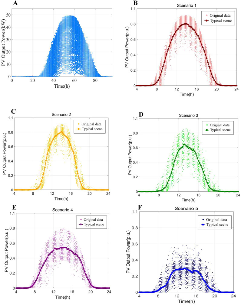
Figure 10. Typical daily output scenario diagram for differentiation. (A) PV annual time series output scenario diagram. (B) Typical scenario 1. (C) Typical scenario 2. (D) Typical scenario 3. (E) Typical scenario 4. (F) Typical scenario 5.

As shown in Figure 10A, the distributed PV output is intermittent, random, and clearly periodic. The power curve generally takes on a half-envelope shape, and its output is positively correlated with sunlight. Due to the influence of solar radiation and temperature, the PV output power curve varies significantly from day to day and has seasonal characteristics. According to the scenario generation process in Figure 5, the 1-year time series output scenario is clustered with the optimal number of clusters.

As shown in Figure 10, after clustering the typical scenarios, the overall difference in the PV output power curve is more obvious, while still retaining the original characteristics. The corresponding output period is 8:00–20:00, with a maximum value between 13:00–15:00, and zero output during the night. This clustering result can be compared to the different scenarios in daily life, such as sunny, cloudy, and rainy days. While maintaining the original diversity of scenarios, it ensures the accuracy of the load calculation to a certain extent and improves the calculation efficiency. Among them, the power curves of scenarios 1 and 2 are relatively stable and have a strong regularity. During these times, there is less cloud cover, and the light and temperature are stable. However, the power changes in scenarios 3, 4, and 5 are more drastic; the curves have more glitches, there is no obvious regularity, and the output power is more random. This clustering result shows that the output power of PV systems varies under different climate types, and the impact of climate on power generation should be fully considered.

5.2 PV power prediction model analysis

To assess the efficacy of the CNN-GRU deep learning prediction model, the PV data for 2023 from a region of Xinjiang Province, China, were employed for verification purposes. Based on the analysis of meteorological influencing factors presented in Section 2.2, solar radiation, ambient temperature, and humidity were identified as the climatic characteristics of primary interest. Subsequently, the training set and test set were divided into a 7:3 ratio according to the five differentiated scene types, following the clustering of the scenes. Power prediction was conducted by the methodology delineated in Section 3.3. The convolutional layer with two steps was used in this process. The 1 × 5 convolutional filter was employed to traverse the two-dimensional PV power generation meteorological characteristics, extracting the relationship between each meteorological characteristic and PV power generation, and then sending the convolutional layer output to the two-layer pooling layer to reduce the dimension and complete feature extraction. A two-layer GRU was constructed, with the number of neurons set to 64 and 128, respectively. The initial power prediction model employed the tanh activation function, and the GRU layer was followed by a fully connected layer that utilized the linear activation function. During the training of the prediction model, the Adaptive Moment Estimation (Adam) optimization algorithm (with a learning rate of 0.001) was used to optimize the model network weight coefficients. The Adam algorithm iteratively updates the weights of the neural network based on the training data, thereby ensuring that the output value of the loss function is optimized (Yi et al., 2020).

As shown in Figure 10, the typical scenarios with a probability of clustering greater than 15% are Scenario 1, Scenario 3, and Scenario 5, which account for 73.5% of the total scenarios. The performance of the three above differentiated scenarios was predicted separately. The typical differentiated scenarios were divided into training and test sets, and the performance was predicted using each deep learning model, as shown in Figure 11.

Figure 11

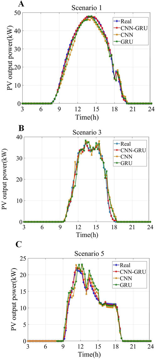
Figure 11. PV prediction results for different scenarios. (A) Typical scenario 1. (B) Typical scenario 3. (C) Typical scenario 5.

As illustrated in Figure 11, among the models, the CNN-GRU model exhibits the highest degree of fit between the PV power prediction curve and the actual PV curve. In scenario 1, the original data set has less fluctuation, the data are clearly regular, and the predicted value is very close to the actual value. In scenarios 3 and 5, the power fluctuation is more obvious, and the prediction curves of the single CNN and GRU models show a certain deviation from the actual values, while the CNN-GRU hybrid model demonstrates a higher degree of fit. Comparing the three differentiated scenarios after clustering in Figure 11, it can be seen that the prediction results of the CNN-GRU model in the differentiated scenarios are more consistent with the actual power changes, and the prediction values are less different from the actual values, better predicting the changes in PV power, thus proving the superiority of the proposed clustering deep learning model.

To further verify the effectiveness of the proposed hybrid deep learning model for PV power prediction, the Mean Absolute Error (MAE), Root Mean Square Error (RMSE) and Mean Absolute Percentage Error (MAPE) were used to evaluate the prediction results. The calculation formulas are as Equations 21–23 (Fan et al., 2020):

$\text{MAE}=\frac{1}{N}{\displaystyle \sum _{i=1}^N}\left|y_i-{\widehat{y}}_i\right|(21)$

$\text{RMSE}=\sqrt{\frac{1}{N}{\displaystyle \sum _{i=1}^N}{\left(y_i-{\widehat{y}}_i\right)}^2}(22)$

$\text{MAPE}=\frac{100}{N}{\displaystyle \sum _{i=1}^N}\left|\frac{y_i-{\widehat{y}}_i}{y_i}\right|(23)$

where ${\widehat{y}}_i$ represents the predicted value; y_i represents the actual value; N is the number of samples.

After data simulation analysis, the evaluation index values of each algorithm are shown in Table 2.

Table 2

Table 2. Summary of the error values of the algorithms.

Further comparisons show that the CNN-GRU model achieves the lowest evaluation metric values across different models and different scenarios, achieving good results in evaluation metric values. Compared to a single model, the prediction accuracy has been significantly improved. Among them, in Scenario 4, the MAE, RMSE, and MAPE of the proposed method were reduced by 29.95%, 28.95, and 24.92%, respectively, compared with the single CNN model, and by 26.1%, 21.9%, and 22.5%, respectively, compared with the single GRU model. Despite the changing weather conditions of Scenario 4 and Scenario 5, the prediction curve of the proposed prediction model still fits the actual value well, and the model is highly practical.

5.3 Analysis of carrying capacity of distribution network with distributed PV

Distributed PV capacity refers to the maximum capacity that can be connected to the grid while ensuring that the power system can operate stably and provide users with a high-quality power supply when the external environment fluctuates. Therefore, the stability of the power system is one of the key factors affecting the load-bearing capacity. The stable operation of the power system depends on a variety of factors, based on the description in Section 4.3, the nodal voltage is identified as an influential factor in the assessment of distributed PV carrying capacity. This paper uses the node voltage of the distribution network as the basis and employs the principle that the node voltage does not exceed the limit to predict and evaluate the load-bearing capacity of distributed PV.

Based on the distributed PV power prediction model constructed in Section 4, firstly, the improved K-means clustering algorithm is utilized to generate PV-differentiated scenarios. Then, the distributed PV power prediction model is constructed using historical data and a CNN-GRU deep learning algorithm to predict the PV power output in the future period. Finally, the predicted PV power is used as the input parameter, and the distribution network power flow calculation method is used to calculate the change in the node voltage of the distribution network after the distributed PV is connected to the grid. By comparing the calculation results with the voltage quality requirements of the distribution network, the distributed PV capacity that can be accessed under the premise of ensuring the safe and reliable operation of the distribution network is determined.

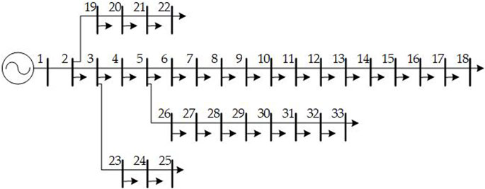
To verify the application performance of the proposed PV power prediction method, the IEEE 33-bus distribution system with distributed PV and load access was selected as the simulation object. After the distributed PV power was predicted, the node voltage after the distributed PV was connected to the grid was obtained. Node 1 was set as the balancing node, and the other nodes were designated as PQ nodes. Figure 12 shows the IEEE 33-bus distribution system.

Figure 12

Figure 12. IEEE 33-bus distribution system topology.

To observe the changes in the voltage of the distribution network nodes after distributed PV was connected to the distribution network, the normalized predicted power of distributed PV in each of the typical scenarios in Section 5.2 was used as the input, and the nodes where PV was connected to the distribution network included nodes 5, 7, 8, 10, 13, 20, 24, 28 and 29. The power of the load nodes was taken as the power curve of a typical weekday for residential loads, with a range of 40%–130%, thereby simulating the system load power consumption from light to heavy. According to historical measured data, the peak photovoltaic power generally arrives around 14:00, and the power is zero before 6:00 and after 19:30. For residential electricity, daytime electricity consumption is high, while before dawn electricity consumption is low, with electricity consumption peaking around 12:00 and 21:00. The time-varying voltage of each node in the distribution network was obtained through power flow calculation. Typical power data for residential loads are shown in Figure 13A, the time-varying voltage of each node in the distribution network under the five differentiated scenarios of distributed PV after clustering are shown in Figures 13B–F.

Figure 13

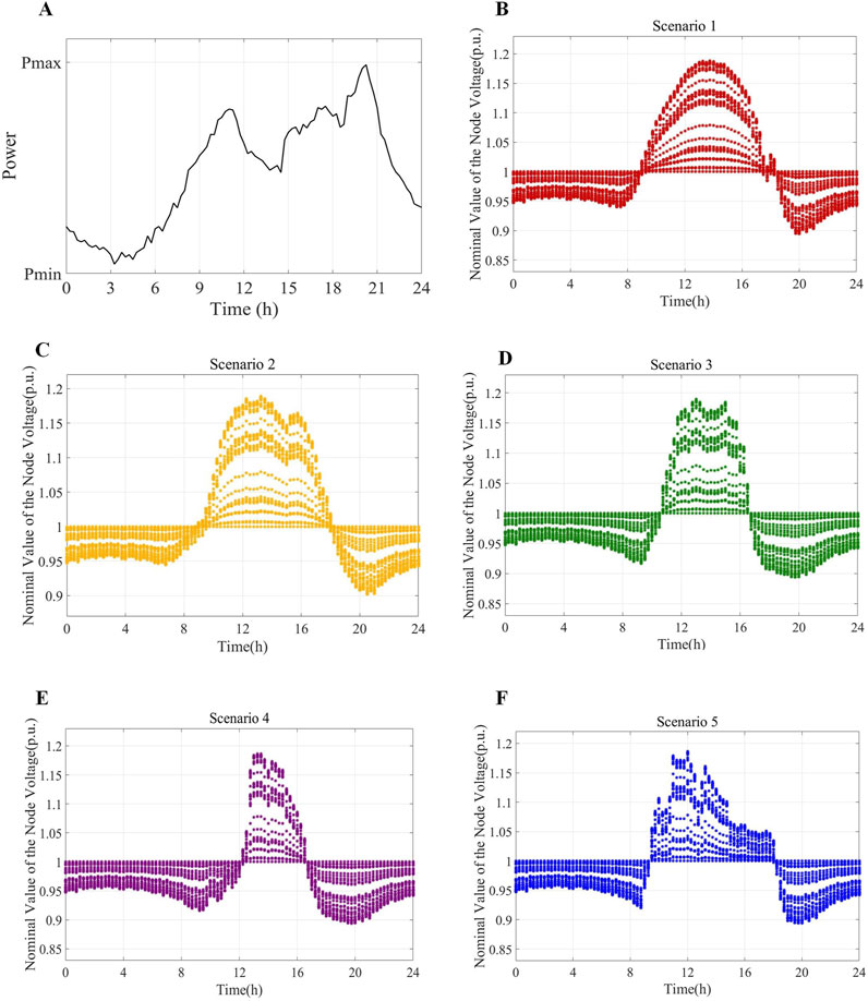
Figure 13. Voltage of time-varying nodes in distribution networks under different scenarios. (A) Residential load power curve. (B) Typical scenario 1. (C) Typical scenario 2. (D) Typical scenario 3. (E) Typical scenario 4. (F) Typical scenario 5.

As illustrated in Figure 13, at approximately 14:00, due to the peak PV power output and relatively small load demand, the voltage at the distribution network node exceeded the standard by as much as 1.19 p. u. According to the relevant standards for the allowable voltage range of the distribution network (Fan et al., 2012), the voltage value at noon had already seriously exceeded the allowable range, and the carrying capacity of the distribution network was low. Particularly when the PV output power is high and the load demand is low, the impact of distributed PV on the node voltage increases. At approximately 20:00, the PV output power was zero and the load power consumption reached a peak. At this time, the node voltage was low, and the load capacity of the distribution network was high. By comparing the different scenarios, the system voltage limit in scenarios 4 and 5 was lower than in scenarios 1 and 2. As sunlight varies, the PV output fluctuates greatly, causing the voltage of the distribution system to fluctuate. By predicting the PV power under differentiated scenarios, the distributed PV time-varying node voltage and carrying capacity of the distribution network can be effectively evaluated, which proves the effectiveness of the proposed CNN-GRU-based PV carrying capacity evaluation model structure.

6 Conclusion and discussions

The high penetration of distributed PV grid-connected power generation has the potential to disrupt the safe and stable operation of distribution networks. To address this challenge, a differentiated scenario-based distributed PV capacity prediction and assessment method based on CNN-GRU deep learning was proposed. The proposed method was verified using measured data from the IEEE 33-bus distribution system. The following conclusions can be drawn from this work:

1. The meteorological characteristics of PV power generation were quantified using the Pearson correlation coefficient method, and the principal meteorological factors influencing PV power were extracted, providing a robust data foundation for PV power generation prediction and capacity research.

2. Considering the difficulty of prediction due to the seasonality and instability of the PV historical data, a differentiated scenario clustering method based on improved K-means clustering and hierarchical clustering was proposed to further simplify the PV uncertain power prediction model and improve the efficiency of calculating the carrying capacity of the distribution network. The simulation results show that the proposed method can effectively cluster the PV output scenarios, and the clustered scenarios are significantly representative. Using the clustered scenarios and probabilities as the calculation scenarios for the study of the load-bearing capacity of the distribution network greatly reduces the amount of calculation while ensuring the accuracy of the calculation.

3. Given the data characteristics of distributed PV and the current PV power prediction method, which faces the problems of insufficient feature extraction and low prediction model accuracy when handling a large amount of data, a PV power prediction model based on improved K-means clustering and CNN-GRU deep learning network was proposed. The model fully considers the temporal and spatial characteristics of PV data, and the simulation results show that the proposed hybrid model achieves higher prediction accuracy than the single model.

4. Combining the time-varying node voltage of the distribution network after PV connection, the proposed PV power prediction strategy under different scenarios was applied to the distribution network, and a method for evaluating the carrying capacity of the distribution network considering different PV scenarios was proposed. The effectiveness of the strategy in evaluating the carrying capacity of the distribution network was verified, providing theoretical guidance for the large-scale integration of distributed PV.

Taking into account the dynamic probabilistic characteristics of multi-source load storage, future research will further study the dynamic probabilistic characteristics of multi-source load storage, and combine it with deep learning methods to analyze the impact of uncertain distributed energy access on the carrying capacity of the distribution network. By establishing a suitable probabilistic model, the uncertainty of multi-source load storage can be more accurately described, and its impact on the carrying capacity of the distribution network can be predicted, guiding the economic operation and daily management of the power system.

Data availability statement

The original contributions presented in the study are included in the article/supplementary material, further inquiries can be directed to the corresponding author.

Author contributions

LZ: Conceptualization, Funding acquisition, Methodology, Project administration, Supervision, Writing–original draft. ZL: Data curation, Formal Analysis, Investigation, Visualization, Writing–review and editing. ZY: Resources, Software, Visualization, Writing–review and editing. ZP: Investigation, Methodology, Visualization, Writing–review and editing.

Funding

The author(s) declare that financial support was received for the research, authorship, and/or publication of this article. The work was supported by State Grid Corporation of China Science and Technology Program under contract no. 5108-202318054A-1-1-ZN titled “Research and application of data-driven intraday forward-looking scheduling technology for key transmission channels.”

Conflict of interest

Authors LZ and ZL were employed by Gird Dispatch Control Center, State Grid Jiangsu Electric Power Company.

Authors ZY and ZP were employed by State Grid Jiangsu Electric Power Research Institute.

The authors declare that this study received funding from State Grid Corporation of China. The funder had the following involvement in the study: inspiring the study design, providing basic data collection and practical engineering scenario description.

Publisher’s note

All claims expressed in this article are solely those of the authors and do not necessarily represent those of their affiliated organizations, or those of the publisher, the editors and the reviewers. Any product that may be evaluated in this article, or claim that may be made by its manufacturer, is not guaranteed or endorsed by the publisher.

References

Antonanzas, J., Osorio, B., Escobar, R., Urraca, R., Martinez-de-Pison, F. J., and Antonanzas-Torres, F. (2016). Review of photovoltaic power forecasting. Sol. Energy 136, 78–111. doi:10.1016/j.solener.2016.06.069

CrossRef Full Text | Google Scholar

Bucciarelli, L. (1986). The effect of day-to-day correlation in solar radiation on the probability of loss-of-power in a stand-alone photovoltaic energy system. Sol. Energy 36 (1), 11–14. doi:10.1016/0038-092x(86)90054-x

CrossRef Full Text | Google Scholar

Chen, W., He, Y., Liu, J., Yang, J., Zhang, K., and Luo, D. (2023). Photovoltaic power prediction based on sliced bidirectional long short term memory and attention mechanism. Front. Energy 11, 1123558. doi:10.3389/fenrg.2023.1123558

CrossRef Full Text | Google Scholar

Cheng, L., Zang, H., Trivedi, A., Srinivasan, D., Wei, Z., and Sun, G. (2024). Mitigating the impact of photovoltaic power ramps on intraday economic dispatch using reinforcement forecasting. IEEE Trans. Sustain. Energy 15 (1), 3–12. doi:10.1109/TSTE.2023.3261444

CrossRef Full Text | Google Scholar

Dolara, A., Leva, S., and Manzolini, G. (2015). Comparison of different physical models for PV power output prediction. Sol. Energy 119, 83–99. doi:10.1016/j.solener.2015.06.017

CrossRef Full Text | Google Scholar

Fan, C., Sun, Y., Xiao, F., Ma, J., Lee, D., Wang, J., et al. (2020). Statistical investigations of transfer learning-based methodology for short-term building energy predictions. Appl. Energy 262, 114499. doi:10.1016/j.apenergy.2020.114499

CrossRef Full Text | Google Scholar

Fan, Y., Zhao, B., Jiang, Q., and Cao, Y. (2012). Peak capacity calculation of distributed photovoltaic source with constraint of over-voltage. Automation Electr. Power Syst. 36 (17), 40–44. doi:10.3969/i.issn.1000-1026.2012.17.008

CrossRef Full Text | Google Scholar

Fernández, Z., Galan, N., Marquina, D., Martinez, D., Sanchez, A., López, P., et al. (2020). Photovoltaic generation impact analysis in low voltage distribution grids. Energies 13 (17), 4347. doi:10.3390/en13174347

CrossRef Full Text | Google Scholar

Fu, L., Yang, Y., Yao, X., Jiao, X., and Zhu, T. (2019). A regional photovoltaic output prediction method based on hierarchical clustering and the mRMR criterion. Energies 12 (20), 3817. doi:10.3390/en12203817

CrossRef Full Text | Google Scholar

Ganti, P., Naik, H., and Barada, M. (2022). Environmental impact analysis and enhancement of factors affecting the photovoltaic (PV) energy utilization in mining industry by sparrow search optimization based gradient boosting decision tree approach. Energy 244, 122561. doi:10.1016/j.energy.2021.122561

CrossRef Full Text | Google Scholar

Ge, J., Cai, G., Yang, M., Jiang, L., Hong, H., and Zhao, J. (2023). Short-term prediction of PV output based on weather classification and SSA-ELM. Front. Energy 11, 1145448. doi:10.3389/fenrg.2023.1145448

CrossRef Full Text | Google Scholar

Haghdadi, N., Bruce, A., MacGill, L, I., and Passey, R. (2018). Impact of distributed photovoltaic systems on zone substation peak demand. IEEE Trans. Sustain. Energy 9 (2), 621–629. doi:10.1109/TSTE.2017.2751647

CrossRef Full Text | Google Scholar

Huang, H., Wang, J., Xiao, Y., Liang, J., Guo, J., and Ma, Q. (2024). Key technologies and research framework for the power and energy galance analysis in new-type power systems. Electric Power Construction 45 (9), 1–12. doi:10.12204/j.issn.1000-7229.2024.09.001

CrossRef Full Text | Google Scholar

Jang, H., Bae, K., Park, H., and Sung, D. (2016). Solar power prediction based on satellite images and support vector machine. IEEE Trans. Sustain. Energy 7 (3), 1255–1263. doi:10.1109/TSTE.2016.2535466

CrossRef Full Text | Google Scholar

Jebli, I., Belouadha, F., Kabbaj, M., and Tilioua, A. (2021). Prediction of solar energy guided by pearson correlation using machine learning. Energy 224, 120109. doi:10.1016/j.energy.2021.120109

CrossRef Full Text | Google Scholar

Jia, K., Gu, C., Xuan, Z., Li, L., and Lin, Y. (2018). Fault characteristics analysis and line protection design within a Large-Scale photovoltaic power plant. IEEE Trans. Smart Grid 9 (5), 4099–4108. doi:10.1109/TSG.2017.2648879

CrossRef Full Text | Google Scholar

Juan, Y., Huang, Z., Hu, C., and Cao, W. (2024). “Overview of photovoltaic power forecasting methods,” in 2024 IEEE 7th International Electrical and Energy Conference (CIEEC), Harbin, China, 10-12 May 2024, 4846–4852. doi:10.1109/CIEEC60922.2024.10583510

CrossRef Full Text | Google Scholar

Kanungo, T., Mount, D., Netanyahu, N., Piatko, C., Silverman, R., and Wu, A. (2002). An efficient k-means clustering algorithm: analysis and implementation. IEEE Trans. Pattern Analysis Mach. Intell. 24 (7), 881–892. doi:10.1109/TPAMI.2002.1017616

CrossRef Full Text | Google Scholar

Li, P., Gu, W., Long, H., Cao, G., Cao, Z., Xu, B., et al. (2019). High-Precision dynamic modeling of Two-Staged photovoltaic power station clusters. IEEE Trans. Power Syst. 34 (6), 4393–4407. doi:10.1109/TPWRS.2019.2915283

CrossRef Full Text | Google Scholar

Li, Y., Su, Y., and Shu, L. (2014). An ARMAX model for forecasting the power output of a grid connected photovoltaic system. Renew. Energy. 66, 78–89. doi:10.1016/j.renene.2013.11.067

CrossRef Full Text | Google Scholar

Li, Y., Sun, Y., Wang, Q., Li, K., and Zhang, Y. (2023). Probabilistic harmonic forecasting of the distribution system considering Time-Varying uncertainties of the distributed energy resources and electrical loads. Appl. Energy 329, 120298. doi:10.1016/j.apenergy.2022.120298

CrossRef Full Text | Google Scholar

Pan, K., Chen, Z., Lai, C., Xie, C., Wang, D., Li, X., et al. (2022). An unsupervised data-driven approach for behind-the-meter photovoltaic power generation disaggregation. Appl. Energy 309 (1), 118450. doi:10.1016/j.apenergy.2021.118450

CrossRef Full Text | Google Scholar

Succetti, F., Rosato, A., Araneo, R., and Panella, M. (2020). Deep neural networks for multivariate prediction of photovoltaic power time series. IEEE Access 8, 211490–211505. doi:10.1109/ACCESS.2020.3039733

CrossRef Full Text | Google Scholar

Theocharides, S., Makrides, G., Livera, A., Theristis, M., Kaimakis, P., and Georghiou, G. (2020). Day-ahead photovoltaic power production forecasting methodology based on machine learning and statistical post-processing. Appl. Energy 268, 115023. doi:10.1016/j.apenergy.2020.115023

CrossRef Full Text | Google Scholar

Wang, H. (2020). Study on optimal methods for enhancing flexibility and resilience of distribution network. Tianjin: University of. [dissertation/doctor's thesis]. Tianjin (CHN).

Google Scholar

Wang, J., Yu, Z., Kong, W., Gao, Y., Zhang, H., and Fu, X. (2022). Multi-Time-Scale analysis of power balance considering coordination between distributed and centralized PV power generation. Front. Energy 10, 902779. doi:10.3389/fenrg.2022.902779

CrossRef Full Text | Google Scholar

Wang, Q., and Lin, H. (2023). Ultra-short-term PV power prediction using optimal ELM and improved variational mode decomposition. Front. Energy 11, 1140443. doi:10.3389/fenrg.2023.1140443

CrossRef Full Text | Google Scholar

Xiao, J., Ye, M., Wang, F., Shen, J., and Gao, F. (2022). Comprehensive evaluation index system of distribution network for distributed photovoltaic access. Front. Energy 10, 892579. doi:10.3389/fenrg.2022.892579

CrossRef Full Text | Google Scholar

Xie, H., Randall, M., and Chau, K. (2022). Green roof hydrological modelling with GRU and LSTM networks. Water Resour. Manag. 36, 1107–1122. doi:10.1007/s11269-022-03076-6

CrossRef Full Text | Google Scholar

Xie, X., Ding, Y., Sun, Y., Zhang, Z., and Fan, J. (2024). A novel time-series probabilistic forecasting method for multi-energy loads. Energy 306, 132456. doi:10.1016/j.energy.2024.132456

CrossRef Full Text | Google Scholar

Yi, D., Ahn, J., and Ji, S. (2020). An effective optimization method for machine learning based on ADAM. Appl. Sci. 10 (3), 1073. doi:10.3390/app10031073

CrossRef Full Text | Google Scholar

Zhang, W., Li, Q., and He, Q. (2022). Application of machine learning methods in photovoltaic output power prediction: a review. J. Renew. Sustain. Energy 14, 022701. doi:10.1063/5.0082629

CrossRef Full Text | Google Scholar

Zhang, X., Wu, Y., Wang, Y., Lv, Z., Huang, B., Yuan, J., et al. (2024). Prediction of photovoltaic power generation based on a hybrid model. Front. Energy 17, 1411461. doi:10.3389/fenrg.2024.1411461

CrossRef Full Text | Google Scholar

Zhen, Z., Pang, S., Wang, F., Li, K., Li, Z., Ren, H., et al. (2019). Pattern classification and PSO optimal weights based sky images cloud motion speed calculation method for solar PV power forecasting. IEEE Trans. Industry Appl. 55 (4), 3331–3342. doi:10.1109/TIA.2019.2904927

CrossRef Full Text | Google Scholar