Transient voltage stability assessment and margin calculation based on disturbance signal energy feature learning

With the increasing variation of the network topology and the high complexity of the processing measurement data, the transient voltage stability assessment of the new power system is facing significant challenges in low accuracy and high time costs. To address the shortcomings of the existing method and apply it to online assessment, this paper proposes an assessment method based on feature learning for disturbance signal energy (DSE) from bus voltages. Firstly, the relationship between DSE and system transient voltage stability is established, and the calculation of DSE from bus voltage time series is detailed. Subsequently, a transient voltage stability assessment method based on the ID3 Decision Tree algorithm and DSE is proposed. Finally, by employing the Support Vector Machine (SVM) to construct the optimal boundary in the feature space formed by the key buses, the transient voltage stability margin (TVSM) for specific scenarios is proposed. Simulation results on the IEEE 39-bus system demonstrate that the proposed method can rapidly and accurately assess the transient voltage stability of the system and calculate the stability margin, providing intuitive and interpretable results with high engineering application value.

1 Introduction

The extensive integration of renewable energy and the widespread application of power electronic equipment in power systems, along with the increase in grid scale and complexity (Gao et al., 2023), has resulted in significant changes to voltage regulation characteristics and reactive power distribution in power grids. This renders the system more susceptible to voltage instability in the event of disturbances. For instance, in January 2023, Pakistan encountered prolonged oscillations and grid splitting as a consequence of substantial wind power generation (Tu et al., 2023). Furthermore, in new power systems, the grid’s topology is highly variable, with frequent maintenance procedures contributing to the complexity of transient voltage stability assessment (Chi and Chen, 2023). Therefore, it is essential to conduct comprehensive research and assessment of transient voltage stability in new power systems to guarantee the safe and reliable operation of the grid.

Early studies on transient voltage stability mainly relied on physical modeling, with time-domain simulation being widely used due to its high adaptability and reliability (La Scala. et al., 1998). However, this method suffers from low computational efficiency and lacks explicit stability criteria (Barab á si and Albert, 1999). To address these shortcomings, Bergen and Hill (1981) introduced the structure-preserving energy function method to the power system, and its effectiveness was validated through numerical simulations. A group of researchers began to apply the energy function method for transient voltage stability assessment later. For instance, Chiang (1989), Overbye et al. (1992a), Overbye et al. (1992b) have proposed frameworks for studying the relationship between voltage stability and energy function. Since then, the energy function method has become a rigorous approach to studying power system stability. Power flow analysis is also crucial in transient voltage stability studies. Kwatny et al. (1986) examined its role in stability loss and voltage collapse bifurcations, while Indulkar et al. (1989) used it to determine voltage stability limits in AC transmission systems. Furthermore, methods based on physical modeling, such as bifurcation theory (Dobson and Chiang, 1989) and trajectory eigenvalue analysis (Pan et al., 2008; Tan et al., 2012), have also been applied. In recent years, with the increasing deployment of various power electronic equipment, challenges have been raised in power system modeling, leading to difficulties in ensuring the accuracy of transient stability analysis based on physical modeling methods (Zhang et al., 2023).

With advances in computer hardware, artificial intelligence technologies, and the maturation of Wide Area Measurement Systems (WAMS), data-driven methods have gradually been applied to voltage stability analysis (Tan et al., 2023; Liu et al., 2024). The application of neural networks in the assessment of transient voltage stability began early (Maeda et al., 1995). Chen and Xie (2022) took the time series of primary measurement data of power systems as the input, and TCN network with attention enhancement module and BiLSTM network were used to extract timing features in parallel to judge the transient voltage stability of the system. Jiang et al. (2014) employed SVM to predict the transient voltage stability condition of the power system, and Niu et al. (2021) achieved the same target by applying AdaBoost-SVM to construct a transient security ensemble learning prediction model. Gao et al. (2022) proposed a voltage stability assessment method in new power systems based on the eGBDT algorithm, which achieved spatial dimensionality reduction. A review of the application of the machine learning methods for transient voltage stability assessment was provided by Adhikari et al. (2020). However, they fall short of intuitively illustrating the physical relationship between transient voltage stability and the observed data, posing challenges for practical engineering applications.

To enhance the interpretability of assessment results, some academics have integrated traditional physical modeling theories with machine learning and treated voltage time series as the object of feature learning. Zhu et al. (2016) and Zhu et al. (2020) assessed transient voltage stability by analyzing time series composed of transient voltages. The relative studies primarily employ the Shapelet method to extract key time-series features from the whole time series. However, the Shapelet methods require substantial computational resources and may suffer the curse of dimensionality when applied to large-scale power grids. In practical engineering, in addition to assessing the transient voltage stability of specific operating scenarios, there is also a significant focus on the stability margin of these scenarios. It is crucial in guiding power system dispatch to ensure safe and stable operation (Wang et al., 2024). The data-driven studies on transient voltage stability rarely provide methods for calculating the stability margin under their respective assessment models.

To address these issues, this paper proposes a transient voltage stability assessment method based on disturbance signal energy (DSE) and the Decision Tree algorithm. The innovations are as follows.

(1) The concept of DSE is introduced. Based on the DSE, the intensity of voltage fluctuations can be more directly reflected compared to the energy function method.

(2) The ID3 Decision Tree algorithm is applied to construct the transient voltage stability assessment model based on DSE. Compared to the Shapelet-based method, the assessment model proposed in this paper shows the advantages of lower time costs and higher interpretability, while maintaining the same level of accuracy.

(3) The optimal decision boundary of the dichotomous samples is obtained using SVM, upon which the stability margin calculation is built. The resulting stability margin provides a definitive assessment of the transient voltage stability and effective guidance for practical dispatching.

The rest of the paper is organized as follows: the concept of transient voltage stability and the definition of DSE are introduced in Section 2. The proposed stability assessment model based on DSE and the Decision Tree algorithm is detailed in Section 3, as well as the margin calculation scheme based on the SVM. A summary of the overall construction process of the model described in Section 3 is provided in Section 4. Results of the tests of the proposed algorithm in this paper on the IEEE 39-bus system are shown in Section 5. The conclusion with a summary of the work presented in the paper is provided in Section 6.

2 Stability problem and energy variation patterns of transient voltage

2.1 Description of transient voltage stability problem

Transient voltage stability refers to the ability of a power system to maintain its voltage level without collapsing and to return to a steady state within a short period after experiencing severe faults or disturbances. Analysis of transient voltage stability typically involves the voltage response and recovery process of the system within a few seconds after the fault occurs (Tang et al., 2002). For a given power system, it can be described by Equation 1:

$\left\{\begin{array}{c}\dot{x}=f\left(x\right)\\ 0=g\left(y\right)\end{array}\right.(1)$

Where: x refers to the state variables in the system, such as angular velocity and power angle, $\dot{x}$ represents the derivative of the variable x with respect to time. The function f(x) describes the dynamic behavior of the system. The variable y is the algebraic variables in the system, such as bus voltages and currents. The function g(y) describes the network equations of the system.

For the dynamic process of the system described by f(x), assume the system operates at a stable equilibrium point x_s, and the corresponding stable region for the system under a certain operation scenario is S(x), with the stable region boundary denoted as $\partial S\left(x\right)$. Traditional transient voltage stability analysis methods assess if the system’s operating point, after a severe disturbance, remains within the stable region boundary $\partial S\left(x\right)$ to determine whether the system voltage will become unstable (Praprost and Loparo, 1994). Based on the stable region, the energy function method can be used to approximate the dynamic process of power systems after a fault (Hou et al., 2004). The energy function method can quickly assess system stability by comparing whether the accumulated energy from the occurrence of the fault to a period after its clearance exceeds the critical energy value corresponding to the stable region boundary. Thus, the problem of determining whether the power system operates within the stable region transforms into the problem of calculating the critical energy of the power system and comparing whether the accumulated energy exceeds the critical energy (Wang et al., 2011).

2.2 Disturbance signal energy method

It is mentioned in Section 2.1 that the energy function method assesses system stability by analyzing the energy accumulation during the transient process. The introduction discusses using artificial intelligence for data-driven analysis to understand power system instability mechanisms. These methods can be combined, employing a simpler yet physically meaningful method of voltage signal energy feature learning to assess the transient voltage stability of a post-fault system.

For the transient voltage stability problem in power systems, analyzing the accumulation of voltage signal energy after disturbances can help judge the likelihood of system instability (Marceau et al., 1996). The calculation method for voltage signal energy is given in Equation 2:

$E={\int }_{t_0}^{t_1}{\left|u\left(t\right)\right|}^{2}dt(2)$

Where: t₀ and t₁ are different time points with t₀<t₁, and u(t) is the curve of voltage over time.

Unlike the traditional energy function method, which calculates system energy primarily based on its actual operating state and topology, the signal energy method directly computes energy through the trend of changes in a specific physical quantity at one bus. While the information contained is relatively less compared to the energy function method, it highlights specific features of interest. For example, in the transient voltage stability of a power system, analyzing the system’s voltage signal energy allows for stability assessment without the need for extensive computations of the system’s overall energy.

Based on Equation 2, the accumulated deviation of the voltage magnitude at a bus from its steady-state value within a short period after a disturbance is defined as the disturbance signal energy (DSE). Considering that in practical calculations, the obtained voltage magnitude data is not an analytical function but a discrete data set, the expression for the voltage DSE is given as Equation 3:

$E={\int }_{t_0}^{t_1}{\left[u\left(t\right)-u\left(0\right)\right]}^{2}dt={\displaystyle \sum _{i=1}^{N_T}}\left[u\left(t_i\right)-u\left(0\right)\right]\Delta t(3)$

Where: u (0) is the steady-state voltage value, N_T is the number of measurement points within the considered period of the time series, Δt is the time interval between two consecutive measurements (i.e., the step size), and u (t_i) is the voltage magnitude corresponding to the ith measurement point.

The voltage DSE can reflect the severity of voltage oscillations during the transient process when a fault or a disturbance occurs. As shown in Figure 1, typical cases of transient voltage stability, critical stability, and instability in the same system after a line fault are presented. The local magnification provides an intuitive reflection of the voltage DSE accumulation at the same bus in these three typical scenarios. The results demonstrate that in the transient process, as the stability decreases, the generated DSE increases. The DSE generated in the stable cases is significantly less than that in the unstable cases. Therefore, DSE can effectively indicate the transient voltage stability of the system.

Figure 1

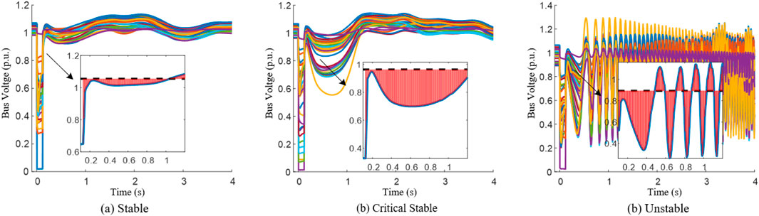
Figure 1. Voltage magnitude time series and its DSE accumulation at different transient stability levels: (A) Stable, (B) Critical Stable, (C) Unstable.

3 Transient voltage stability assessment and margin calculation based on feature learning of disturbance signal energy

3.1 Generation of disturbance signal energy data set

The transient voltage time series data set of a d-dimensional power system is denoted as $S=\left\{S_1,S_2,\dots ,S_d\right\}$, where $S\in {\mathbb{R}}^{n\times d\times N_T}$, n is the number of cases, and N_T is the length of the time-series data, i.e., the number of measurement points. To illustrate the generation of the DSE set, take the dimension i (1 ≤ i ≤ d) of the dataset S as an example. The dataset S_i in dimension i is composed of n time series all of length N_T, as shown in Equation 4.

$S_i=\left\{U_{i,1},U_{i,2},\dots ,U_{i,n}\right\},i=1,2,\dots d(4)$

Where: $U_{i,j}=\left\{u_{i,j}\left(t_1\right),u_{i,j}\left(t_2\right),\dots ,u_{i,j}\left(t_{N_T}\right)\right\}$, j = 1, 2 … , n, and $u_{i,j}\left(t_1\right)$ represents the value of the voltage at bus i for the sample j at the first measurement point.

Each time series can be transformed into the DSE generated over a certain period according to Equation 3. After n time series have been transformed, we can obtain the DSE set for a single bus i, as shown in Equation 5:

$E_i=\left\{E_{i,1},E_{i,2},\dots ,E_{i,n}\right\}(5)$

Each element $E_{i,j}$ in Equation 5 is a scalar that denotes the DSE generated by the voltage at bus i in sample j over the given time series. For sample j, taking $E_{i,j}$ as the feature attribute of bus i, the DSE set $E_i$ for bus i is sorted in ascending order to obtain $E_i^{sort}=\left\{E_{i,1}^{\prime },E_{i,2}^{\prime },\dots ,E_{i,n}^{\prime }\right\}$. Then the average values between each pair of adjacent elements in $E_i^{sort}$ are calculated to obtain the candidate set of split thresholds for the DSE at bus i, denoted as $E_i^{mean\_sort}=\left\{E_{i,1}^{mean},E_{i,2}^{mean},\dots ,E_{i,n-1}^{mean}\right\}$. The operation of sorting and taking the average value of $E_i$ is speedily to select featured system buses with distinct information for stability judgment.

Similarly, by applying the same process to all dimensions (i.e., all the buses in the power system) in S, we can obtain the candidate set of split thresholds for the DSE of multiple buses under a given number of samples, which is used to partition the data set into different subsets, denoted as ${\mathit{E}}^{mean\_sort}$, as shown in Equation 6:

${\mathit{E}}^{mean\_sort}=\left[\begin{array}{cccc}{E}_{1,1}^{mean\_sort}& E_{2,1}^{mean\_sort}& \cdots & E_{d,1}^{mean\_sort}\\ E_{1,2}^{mean\_sort}& E_{2,2}^{mean\_sort}& \cdots & E_{d,2}^{mean\_sort}\\ ⋮& ⋮& \ddots & ⋮\\ E_{1,n-1}^{mean\_sort}& E_{2,n-1}^{mean\_sort}& \cdots & E_{d,n-1}^{mean\_sort}\end{array}\right](6)$

3.2 Construction of the transient stability assessment model based on decision tree

The core idea of the decision tree machine learning method is to partition the data set into different subsets through a series of decision rules (Karabadji et al., 2023). This process is relatively simple and efficient, and the classification model and assessment results are presented in a tree structure, which retains the clear physical significance of the DSE. In this study, different buses in the system under study are defined as different attributes of the corresponding decision tree model. Since the number of buses in each data sample is the same, meaning the number of attributes is consistent across samples, there is no preference for attributes with more or fewer possible values (Li et al., 2020). Therefore, the ID3 Decision Tree algorithm is here applied to construct the transient voltage stability assessment model, using information gain as the criterion for selecting DSE split thresholds at each node during the learning process.

To facilitate the subsequent explanation of information gain, the definition of information entropy is provided first (Omuya et al., 2021). Information entropy refers to the level of disorder in a data set. The more homogeneous the categories within the dataset, the lower the information entropy is. Since this study deals with a binary classification problem for stability assessment, where the samples (described in Equation 5) in E are either stable or unstable, denoted as $C_1$ and $C_2$ , respectively, with their proportions in E being $p_1$ and $p_2$, the degree of disorder in E can be expressed as Equation 7:

$\text{Ent}\left(E\right)=-{\displaystyle \sum _{k=1}^2}\left[p_k{\log }_2\left(p_k\right)\right](7)$

Where: Ent(E) is the information entropy of E.

For each bus of the d-dimensional power system, a candidate energy split threshold $E_i^{divide}$ is randomly selected from $E_i^{mean\_sort}$ to partition E into two subsets, denoted as $E_{less}$ and $E_{greater}$ (where each element in $E_i=\left\{E_{i,1},E_{i,2},\dots ,E_{i,n}\right\}$ of $E_{less}$ in the dimension is less than $E_i^{divide}$, and each element in $E_i=\left\{E_{i,1},E_{i,2},\dots ,E_{i,n}\right\}$ of $E_{greater}$ in the dimension i is greater than $E_i^{divide}$).

To calculate the information entropy of the subsets $E_{less}$ and $E_{greater}$, the number of stable and unstable samples in $E_{less}$ and $E_{greater}$ are counted, respectively. Then, according to Equation 8, the expression for the conditional information entropy after classification is obtained as follows:

${\text{Ent}}_{E_i^{divide}}\left(E\right)=p_{E_{\text{less}}}\times \text{Ent}\left(E_{\text{less}}\right)+p_{E_{\text{greater}}}\times \text{Ent}\left(E_{\text{greater}}\right)(8)$

Where: $p_{E_{\text{less}}}$ and $p_{E_{\text{greater}}}$ are the proportions of the sample numbers of $E_{less}$ and $E_{greater}$ in E, respectively.

Thus, the information gain (IG) obtained by partitioning the data set using $E_i^{divide}$ is as Equation 9:

$\text{IG}\left(E,E_i^{divide}\right)=\text{Ent}\left(E\right)-{\text{Ent}}_{E_i^{divide}}\left(E\right)(9)$

Using Equations 7–9, the candidate energy split threshold with the maximum IG from the n-1 candidate energy split thresholds contained in $E_i^{mean\_sort}$ is selected as the optimal energy split threshold for bus i, set as $E_{i,\max }^{mean\_sort}$ . Similarly, the optimal energy split thresholds for all buses in the system are obtained. By comparing the information gains corresponding to the optimal energy split thresholds of multiple buses, select the bus with the maximum information gain and its energy split threshold as a decision tree node. The $E_{less}$ or $E_{greater}$ corresponding to $E_{i,\max }^{mean\_sort}$ is further used to find the next decision tree node by updating Equations 6–9. The following outlines the specific process for generating the decision tree model based on DSE.

As shown in Figure 2, the decision tree model classifies through multiple layers of if-then rules. After inputting the candidate set of energy split thresholds, $E^{mean\_sort}$, into the decision tree, the decision tree model starts from the root node and compares the data of each dimension in the input DSE set. Based on the predetermined rules, the information gain is calculated and the attribute (i.e., the DSE of bus voltage) and the corresponding split threshold with the best classification performance are selected as the root or internal node. This ensures that the binary branches generated from this node maximize the number of similar samples in the corresponding sample subsets while minimizing the number of dissimilar samples, thereby reducing the entropy of the sample subsets as much as possible. This process of recursively optimal partitioning of the data set continues until each sample subset contains only similar samples or the number of samples in a subset reaches a preset threshold, at which point the tree stops growing. Finally, the corresponding label of similar samples or the majority label of dominant samples is stored in the terminal leaf nodes as the classification label. Ultimately, all branches, internal nodes, and leaf nodes from the root node are integrated into a complete decision tree structure.

Figure 2

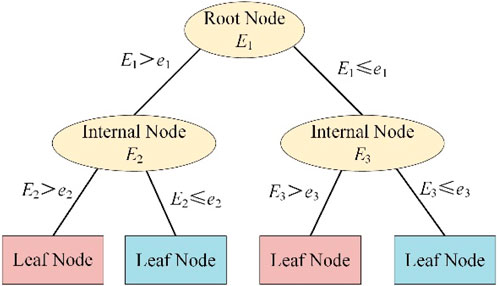
Figure 2. Schematic diagram of the decision tree model.

When significant changes occur in the topology of power systems, the DSE set can be rapidly generated, as the generation process of the DSE set involves direct function transformation without a search process as the Shapelet-based method, allowing new thresholds to be quickly learned from the new DSE set. Due to these advantages, the method proposed in this paper demonstrates higher adaptability and practicality in real power grids.

After assessing transient voltage stability using a binary classification decision tree model based on DSE feature learning, the resulting stable or unstable labels prove insufficient for effectively guiding the scheduling, operation, and maintenance processes of the power system. To more intuitively demonstrate the system’s stability under a certain scenario, the attributes contained in the nodes of the decision tree model, which correspond to the system buses in this paper, are considered the key buses that have the greatest impact on transient voltage stability in the studied system. These key buses are then used to construct a transient voltage stability margin calculation model.

3.3 SVM-based transient voltage stability margin calculation

As mentioned above, the fluctuation of bus voltage magnitude after the system is disturbed can be reflected through DSE. In a specific scenario, the disturbance severity of each bus in the system is positively correlated with each other (Hou et al., 2015), then the DSE generated by the voltage of each bus in the system will show the phenomenon of “increasing and decreasing simultaneously”, and the larger the DSE generated by the system after a fault, the more likely that the system voltage will undergo transient instability (Odun-Ayo and Crow, 2012). Therefore, in the feature space $\mathbb{E}$ composed of the DSE generated by the voltage of the key buses, the sample points corresponding to different scenarios will show an approximate linear distribution, and then SVM can be used to obtain the approximate linear boundary between the stable samples and unstable samples to construct the stability margin calculation model (Tan et al., 2024).

The essence of SVM is to find the hyperplane in the feature space that maximizes the interval between the dichotomous samples. The sample set E is divided into stable sample set, E_.g., and unstable sample set E_b by the classification of the decision tree model, and the two types of samples are assigned the stable labels y = 1 and y = −1. The hyperplane divided by the linear SVM can be expressed as Equation 10:

$\mathit{w}\mathit{s}+b=0(10)$

Where: w denotes the coefficients of the hyperplane, s denotes the variables in the feature space, and b is the bias term.

In practice, normal samples are often contaminated by a small number of abnormal samples, leading to errors. To solve it, slack variables are introduced, and the optimal values of w and b can be obtained by solving the optimization problem in Equation 11:

$\left\{\begin{array}{l}\min \frac{1}{2}{‖\mathit{w}‖}^2+C{\displaystyle \sum _{i=1}^l}{\xi }_i\\ s.t.\left\{\begin{array}{l}{y}_i\left({\mathit{w}\mathit{s}}_i+b\right)\ge 1-{\xi }_i\\ {\xi }_i>0\end{array}\right.,i=1,2,\cdots ,l\end{array}\right.(11)$

Where: y_i denotes the stability label of the training sample; ${\xi }_i$ is the slack variable; $C$ is the penalty factor, used to control the degree of punishment for misclassification, l is the number of variables in the feature space.

After the boundary equation with the maximum distance between two types of samples is obtained using SVM, the transient voltage stability margin (TVSM) of a specific scenario corresponding to the sample can be calculated based on the distance from the sample’s DSE to the boundary in the space $\mathbb{E}$.

The ideal situation where the voltage magnitude curve at each bus can immediately and vertically return to a steady state after fault clearance is taken as the baseline for normalizing the stability margin. In this case, the DSE generated at each bus is 0. Thus, the TVSM of the system under a certain scenario is defined as Equation 12:

$\left\{\begin{array}{c}\begin{array}{l}\text{TVSM}\left(E_j\right)=\left\{\begin{array}{l}\frac{D_{\text{st}}\left(E_j\right)}{D_{\text{Ref}}},E_j\in E_g\\ \frac{-D_{\text{st}}\left(E_j\right)}{D_{\text{Ref}}},E_j\in E_b\end{array}\right.\\ D_{\text{st}}\left(E_j\right)=\frac{\left|\left(E_j•\mathit{e}\right)+b\right|}{‖\mathit{e}‖}\end{array}\\ D_{\text{Ref}}=\max \left\{\underset{E_j\in E_g}{\max }{D}_{\text{st}}\left(E_j\right),D_{\text{st}}\left(0\right)\right\}\end{array}\right.(12)$

Where: E_j refers to the sample j in the stable sample set, E_.g., D_st (E_j) refers to the perpendicular distance from sample j to the optimal boundary, e is the normal vector of the optimal boundary in the feature space, b is the constant term of the hyperplane equation, D_Ref is the reference distance value, $\underset{E_j\in E_g}{\max }{D}_{\text{st}}\left(E_j\right)$ represents the maximum value among the perpendicular distances from all samples E_j in the sample set, E_.g., to the optimal boundary, and D_st (0) refers to the perpendicular distance from the origin to the optimal boundary. D_Ref is chosen as the maximum value of D_st (E_.g.,) and D_st (0) to ensure that the calculated TVSM will not exceed 1.

After the stability margins corresponding to the scenarios of all samples in the sample set are calculated, the transient voltage stability level of the system after fault clearance is categorized into three types: stable, critically stable, and unstable, as shown in Table 1. Unlike the commonly used definition that considers samples that reach the limit of stability as critical samples, which is not instructive, in this paper, the stable samples with their TVSM ranked within the bottom 5% are considered as the critical samples (Li et al., 2019), and the maximum TVSM value among these critical samples is defined as the division $\eta$. 5% is an empirical value, the value of $\eta$ can be adjusted according to actual operating requirements. When TVSM = 1, the system is in an ideal stable state, where the voltage curve can immediately return to steady-state after fault clearance, without any overshoot or oscillation. When TVSM = 0, according to Equation 12, the sample point lies on the optimal boundary, and the system is exactly at the critical point between stability and instability. Considering that engineering design and operation usually adopt a conservative strategy, this paper classifies the samples with TVSM = 0 as unstable.

Table 1

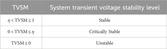
Table 1. Division of transient voltage stability margin.

4 Implementation of the overall scheme

Based on the decision tree model learned from perturbation signal energy characteristics and the transient voltage stability margin calculated by the perpendicular distance between the SVM optimal boundary and sample points, the overall scheme for assessing transient voltage system stability and calculating the margin is shown in Figure 3.

Figure 3

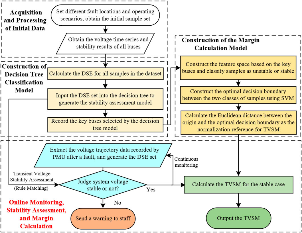
Figure 3. Overall scheme of transient voltage stability assessment and margin calculation.

The overall scheme is implemented in four stages.

(1) Initial Data Acquisition and Processing: For a given system, considering its various possible operating conditions and fault types, a large number of simulation cases are generated through transient numerical simulations. The voltage time series is transformed into the DSE generated during the given period using Equation 3. The transformation completes the conversion from the time series dataset to the DSE dataset, preparing for subsequent learning.

(2) Construction of Decision Tree Classification Model: Based on the DSE dataset generated in the previous stage, the ID3 Decision Tree algorithm is applied to learn from these data and generate a decision tree classification model for transient voltage stability assessment. Each node in the tree corresponds to the DSE and its splitting threshold for the respective bus, which is considered the key bus of the power system. These key buses form the foundation for subsequent calculations of the TVSM based on SVM.

(3) Construction of the Margin Calculation Model: Based on the key buses obtained in step (2), a d-dimensional disturbance signal energy feature space $\mathbb{E}$ is constructed. After classification by the decision tree model, the sample points are labeled as stable and unstable. Using SVM, an approximate optimal linear boundary between the stable and unstable samples is obtained. The distance from each sample point to the optimal boundary is then used to calculate the TVSM of the corresponding scenario.

(4) Online Monitoring, Stability Assessment, and Margin Calculation: When the system undergoes a severe disturbance, the post-fault voltage time series data from the PMU is converted into a DSE dataset. This dataset is used for top-down path searching in a decision tree model. Upon reaching a leaf node, the node’s class label provides the assessment result. If the system is judged to be unstable, an alarm signal will be immediately issued to alert the operating personnel to take control measures. If the result shows to be stable, the TVSM under the given fault will be calculated, thereby providing better guidance for personnel in the dispatch.

5 Case study

To verify the validity and superiority of the proposed method, the New England 10-machine 39-bus system (IEEE 39-bus system) with wind power access is built in DIgSILENT software, as shown in Figure 4. The locations of wind farms integrated into the system and the specific configurations of the wind turbine generators can be found in the Appendix.

Figure 4

Figure 4. Single line diagram of IEEE 39-bus system with wind power farms.

Both the training and test set in the case study are obtained by transient simulation through DIgSILENT software. To enrich the diversity of the scenarios, the load size and synchronous machine output are adjusted based on the standard operation scenario of the system, and the Monte Carlo method is applied to simulate the stochastic nature of wind power output. The implementation plan is detailed in the Appendix. Meanwhile, considering the N-1 and N-2 principles, 1 or 2 important lines will be randomly disconnected in the case study before setting the faults according to the above schemes.

Under these conditions, the initial data samples are generated by transient numerical simulation, and then the voltage magnitude time series at each bus are extracted as the needed data samples. Taking the fault clearing time as the starting point, given the time window T to be 0.8 s, the sampling interval $\Delta t$ is set to be 0.01 s, the same as the simulation time step. The time window is utilized to extract the time series of the voltage magnitude per unit value at each bus. The length of each time series is $m=T/\Delta t$.

5.1 Stability assessment model utility verification and performance analysis

In this section, 1,200 data samples are generated through transient numerical simulations. Of these, 800 are randomly selected for offline training of the proposed method to construct the stability assessment model, while the remaining 400 are used to test the model construction efficiency and classification accuracy of the method. From the training samples, a candidate DSE set is generated, and the ID3 Decision Tree is used to train the candidate set for classification, resulting in the decision tree classification model shown in Figure 5. Taking the root node in the figure as an example, E_Bus5 denotes the DSE generated by the voltage at Bus 5 within time T after fault clearance, and the attributes of the feature variables on the rest of the nodes are similar to this one. The class labels on the leaf nodes indicate stability judgment results, with −1 and 1 representing instability and stability, respectively. A 10-fold cross-validation is used to test the accuracy of the constructed classification model, yielding a cross-validation accuracy of 99%, indicating that the model has excellent classification performance.

Figure 5

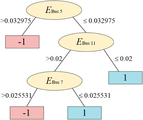
Figure 5. Decision tree classification model.

Considering the particularity of transient voltage stability classification: the costs of misclassifying instability as stability (false negatives) and stability as instability (false positives) are significantly different. The former can easily lead to irreversible voltage collapse or even power outages, resulting in substantial economic losses, while the latter can typically be remedied in time with corrective control measures, leading to much smaller losses. Given the same probability of misclassification, system operators prefer to classify samples as unstable to avoid severe, irreversible consequences. Therefore, in subsequent comparisons of different algorithm performances, both the false negative rate and false positive rate are used as evaluation metrics (Zhu et al., 2016). When applying data mining methods to transient voltage stability analysis, considering the conservative nature of power system operation, it is important to not only improve classification accuracy (i.e., reduce the total number of false negatives and false positives) but also to minimize the total number or proportion of false negatives (Dai et al., 2015).

When using the resulting decision tree classification model to assess transient voltage stability online, the WAMS first collects the voltage time series of buses 5, 11, and 7 within time T after fault clearance. Then, the DSE generated by these time series compared to their steady-state values is calculated and compared with the splitting thresholds in the model in a top-down sequence until a leaf node is encountered, then the stability discrimination result can be obtained. By employing this approach, the remaining 400 samples that were not used in training are tested to simulate online monitoring and stability assessment, further validating the model’s classification performance. The results show an overall accuracy rate (AR) of 99%, with a false positive rate (FPR) of 1% and a false negative rate (FNR) of 0%. It proves that the classification model can be reliably and effectively used for online monitoring.

Under the same conditions of parameters, data samples, and configuration environment, the proposed transient voltage stability assessment model based on DSE feature extraction is compared with the improved algorithm which uses piecewise linear fitting before Shapelet search to avoid inefficient point-by-point sliding search (Ye and Keogh, 2009), and the stability assessment algorithm based on particle swarm optimization to accelerate Shapelet search (Zhu et al., 2016). The aforementioned algorithms are hereafter referred to as Algorithm I, B, and C, in sequence. The comparison results are shown in Table 2.

Table 2

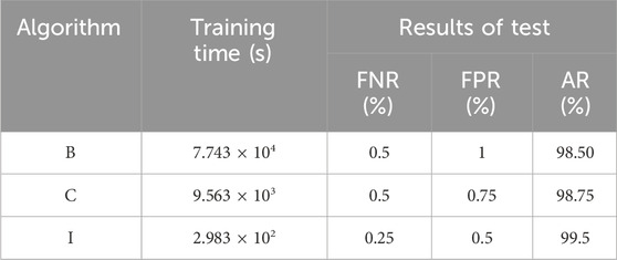
Table 2. Comparison of training time and accuracy of four algorithms.

Compared with algorithms B and C, Algorithm I significantly reduces the training time to less than 300 s. This is because Algorithm I adopts the DSE split threshold which is single-dimensional as the comparison object, while Algorithms B and C first search for the optimal two-dimensional time series and then transform it into a Euclidean distance split threshold for comparison. Algorithm I eliminates the complex optimal subsequence search process, significantly reducing the model training time cost and shows a high degree of flexibility for the rapid updating of the topology and morphology of the power grid.

In terms of accuracy, the proposed algorithm in this paper shows a reduction in both missed detection rates and false alarm rates compared to Algorithms B and C, resulting in an overall improvement in accuracy. By referring to the decision tree classification model shown in Figure 5, the reasons for this improvement are as follows: the DSE of the bus in the stable samples are all less than the energy splitting thresholds of the nodes inside the decision tree, whereas the DSE of unstable samples is all greater than the energy splitting thresholds. It means that the samples have obvious differentiation in the model constructed by Algorithm I. Meanwhile, different types of instability may cause the system’s voltage curves to exhibit various patterns, such as gradual decline, damped oscillation, sustained oscillation, and voltage collapse, which lead to significant differences in the voltage curves shortly after fault clearance. Algorithms A, B, and C evaluate stability by comparing the Euclidean distance between the voltage curve trajectories and an optimal Shapelet. As a result, they may confuse stable and unstable curves when faced with different instability types, leading to misjudgment. The proposed method, by comparing disturbance signal energy levels, overcomes the limitations of shapelet-based methods. Thus achieving higher accuracy. This is also why the proposed algorithm outperforms shapelet-based methods in terms of accuracy.

In practical engineering applications, power grid lines are frequently under maintenance. Therefore, the topology and configuration of the power grid during online monitoring often differ from those during offline training. In such cases, stability assessment models need to have strong robustness and generalization capabilities.

To verify that the proposed method maintains robust stability assessment capabilities even when minor changes occur in the power grid topology due to line maintenance, the following example is set to an extreme condition. In the IEEE 39-bus system shown in Figure 4, the system load levels, outputs of synchronous generators and wind farms, and fault locations are randomly set according to the previously described conditions. Without any line maintenance, 200 data samples (denoted as the training set A1) are obtained through transient numerical simulations for offline training. Then, following the N-2 criterion, two lines are randomly taken out of service, and 800 data samples (denoted as the test set A2) are obtained through simulations for testing. Similarly, 200 new data samples under the N-2 criterion are obtained as a new training set (denoted as the training set B1), and 800 data samples without any line maintenance are obtained as a new test set (denoted as the test set B2). After 10 times of random data extraction, the average results obtained from the test are shown in Table 3.

Table 3

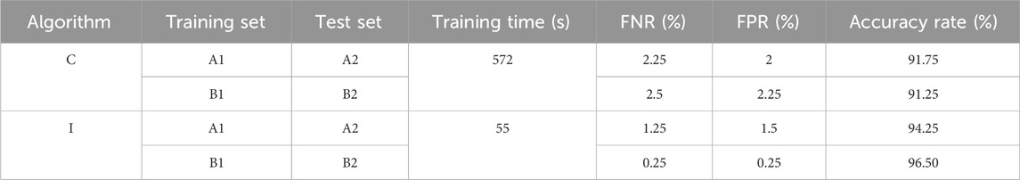
Table 3. Comparison of the performance of the two algorithms in the face of N-2 maintenance and insufficient samples.

From Table 3, it can be observed that the proposed method maintains high accuracy and a low leakage rate even when faced with changes in the power grid’s topology and structure due to line maintenance, as well as insufficient fault samples for training new models in practical engineering scenarios, and its accuracy and model training efficiency are higher than that of the Shapelet-based stability assessment algorithm represented by Algorithm C. This is because when facing the same fault, the bus voltage time series will change due to the different topology of the power grid. At the time, the DSE-based feature learning can be well adapted to this change.

Assuming the system remains transiently stable before and after topology changes, Algorithm I converts time series sets into energy sets, with the core as shown in Equation 3. Each value at a sampled time point is subtracted from the steady-state value, and the square of this difference is multiplied by the simulation step size of 0.01 s. This difference does not change dramatically due to minor trajectory variations.

To further illustrate the critical role of DSE in identifying the trend toward system instability and the effect of the selection of the time window T on the results, 800 samples used for offline training in the example shown in Figure 5 are selected. Bus 5, the root node of the decision tree model, is taken as the observation object, and its time series curve of the DSE generated in 0–1.4 s after fault clearance is shown in Figure 6.

Figure 6

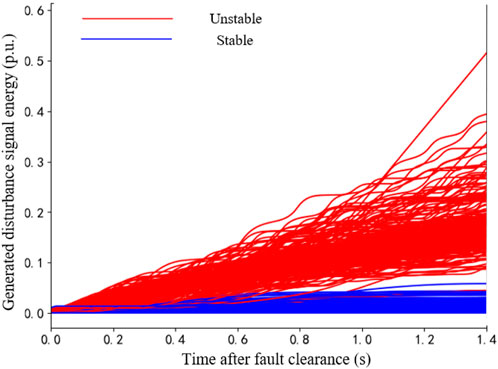
Figure 6. Time series curve of DSE at Bus 5

In Figure 6, as time progresses after fault clearance, the time series curves of DSE for stable samples gradually flatten. At the later stage, the voltage curve returns to the steady state and almost no longer generates DSE. On the other hand, the DSE curve of the unstable samples continues to climb after fault clearance because the voltage curve cannot return to the vicinity of the steady-state value, so the difference in the magnitude of the DSE generated by the bus voltages between the stable samples and the unstable samples becomes increasingly evident.

In the above process, the distinction between the two types of samples becomes increasingly clear after 0.8 s, which means that the longer the time window T after the fault clearance is taken, the more DSE is generated by this time series. The enhanced differentiation between stable and unstable samples results in fewer internal nodes in the constructed decision tree model, which is beneficial to the accuracy of the stability assessment and the subsequent margin calculation. However, the longer the time window T taken for analysis, the less time is left for automated engineering systems to react or for human operators to take corrective actions after the assessment model evaluates that the transient voltage stability will become unstable and issues a warning. This is not conducive to operators taking timely control measures to prevent the instability incident from escalating further.

5.2 Calculation and analysis of transient voltage stability margin

Based on the decision tree classification model obtained in Section 5.1, the decision nodes corresponding to the system buses are identified. In this case, three buses are included, and a three-dimensional feature space is constructed based on the DSE corresponding to these buses.

As mentioned in Section 3.3, the overall DSE of all buses in the system shows a “simultaneously increase or decrease” trend after the system suffers a disturbance. This means that in the feature space, the sample points are roughly concentrated along a line. To verify this conclusion, the distribution of the DSE of the sample points in the feature space is shown below. As illustrated in Figures 7A–C, the sample points are approximately distributed along a straight line on the three cross-sections of the three-dimensional space, with linear fitting degrees of 0.9583, 0.9870, and 0.9613, respectively. This indicates that the sample points are approximately linearly distributed in the three-dimensional space. At this point, SVM can quickly find the optimal classification boundary to perform subsequent stability margin calculations.

Figure 7

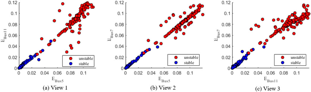
Figure 7. Distribution of sample points in the feature space: (A) View 1, (B) View 2, (C) View 3.

Based on Section 3.3, the calculation of the TSVM is performed by the constructed decision boundary. The accuracy of the calculation is heavily dependent on the precision of the decision tree classification model. To verify that the transient voltage stability of the system is well differentiated in the above feature space constructed by the decision tree model, 800 training samples from the first case study in Section 5.1 are used to train the SVM model. The additional 400 samples are utilized for testing. The optimal decision boundary equation for classifying stable and unstable samples is provided in Equation 13. The SVM model achieves a classification accuracy of 99.25% on the 400 test samples, demonstrating a high level of reliability and accuracy in practical applications. Figure 8 presents the distribution of 400 test samples and the optimal decision boundary in the feature space of key buses. In this figure, the cyan plane represents the optimal decision boundary, blue points indicate stable samples and red points denote unstable samples.

$-8.412E_{Bus5}-8.36E_{Bus11}-7.864E_{Bus7}+1.092=0(13)$

Figure 8

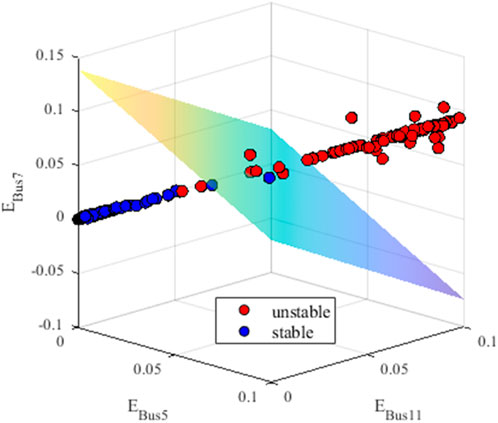
Figure 8. Three-dimensional spatial distribution of the optimal decision boundary and test samples.

Based on Equations 12, 13, the TSVM for 400 data samples is calculated. Using the results presented in Table 1, a subset of samples categorized as transiently stable, critically stable, and unstable are chosen for comparative analysis. According to the definition in Equation 12, the critical TSVM value $\eta$ corresponding to these 400 samples is 0.1652. Based on the resulting $\eta$,the response curves of the voltage magnitudes at each bus within 5 s following a fault for samples of varying stability levels are illustrated in Figure 9.

Figure 9

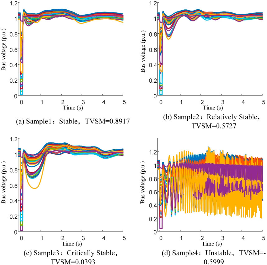
Figure 9. Voltage magnitude response curves for different stability levels: (A) Sample 1, (B) Sample 2, (C) Sample 3, (D) Sample 4.

Based on Figure 9, as the transient voltage stability margin of the system gradually decreases, the amplitude of the voltage magnitude trajectories at various buses increases after the line fault clearance. Initially, the voltage magnitudes exhibit slight oscillations around their steady-state values and quickly become stable. As the stability margin continues to decrease, the oscillations become more pronounced around the steady-state values. Ultimately, when the system becomes unstable, the voltage magnitudes oscillate violently and then diverge.

Sixty sample parameter settings were randomly selected from Figure 8. The corresponding critical clearing times were obtained through iterative testing in DIgSILENT to validate the accuracy of the calculated stability margins. The results are shown in Figure 10. As seen in Figure 10, when the TSVM values of the samples increase, their critical clearing times generally increase as well. The linear fit between the two has a correlation coefficient of 0.8522.

Figure 10

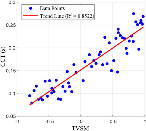
Figure 10. The relationship between the system’s TVSM and CCT.

Based on the results in Figures 8, 10, it is validated that the transient stability margin calculated by the method proposed in this paper effectively reflects the transient voltage stability in practical operating scenarios. The method demonstrates sufficient usability within an acceptable range of error and has the potential for application in engineering practice.

6 Conclusion

This paper focuses on the transient voltage stability assessment of modern power systems, integrating machine learning with the transient voltage trajectory of buses. A transient voltage stability assessment model based on Decision Tree and disturbance signal energy (DSE) is proposed, as well as a stability margin calculation scheme based on SVM. The main contributions and results of this paper are as follows.

(1) The concept of DSE is introduced. Based on the DSE, the intensity of voltage fluctuations can be more directly reflected compared to the energy function method. The ID3 Decision Tree algorithm is applied to construct the transient voltage stability assessment model based on DSE. Compared to the Shapelet-based method, the assessment model proposed in this paper shows the advantages of lower time costs and higher interpretability, while maintaining the same level of accuracy.

(2) The optimal decision boundary of the dichotomous samples is obtained using SVM, upon which the stability margin calculation is built. The resulting stability margin provides a definitive assessment of the transient voltage stability and effective guidance for practical dispatching.

(3) The effectiveness of the proposed transient voltage stability assessment and margin calculation methods is verified through the tests on the IEEE 39-bus system. The case study results show that the proposed method has the advantages of low time cost, high accuracy, and strong robustness, demonstrating significant potential for online monitoring and assessment of transient voltage stability in new power systems.

Data availability statement

The raw data supporting the conclusions of this article will be made available by the authors, without undue reservation.

Author contributions

YC: Writing–original draft, Funding acquisition, Software, Supervision. ZH: Writing–original draft, Writing–review and editing, Conceptualization, Validation. ZD: Writing–original draft, Writing–review and editing, Funding acquisition, Supervision. GZ: Writing–original draft, Writing–review and editing, Conceptualization. JG: Writing–original draft, Writing–review and editing. HZ: Writing–original draft, Software.

Funding

The author(s) declare that financial support was received for the research, authorship, and/or publication of this article. This research was supported by the State Key Laboratory of HVDC, Electric Power Research Institute, China Southern Power Grid (SKLHVDC-2022-KF-14).

Conflict of interest

The authors declare that the research was conducted in the absence of any commercial or financial relationships that could be construed as a potential conflict of interest.

Publisher’s note

All claims expressed in this article are solely those of the authors and do not necessarily represent those of their affiliated organizations, or those of the publisher, the editors and the reviewers. Any product that may be evaluated in this article, or claim that may be made by its manufacturer, is not guaranteed or endorsed by the publisher.

Supplementary material

The Supplementary Material for this article can be found online at: https://www.frontiersin.org/articles/10.3389/fenrg.2024.1479478/full#supplementary-material

References

Adhikari, A., Naetiladdanon, S., Sagswang, A., and Gurung, S. (2020). “Comparison of voltage stability assessment using different machine learning algorithms,” in 2020 IEEE 4th Conference on Energy Internet and Energy System Integration (EI2), Wuhan, China, October 30–November 1, 2020, 2023–2026. doi:10.1109/EI250167.2020.9346750

CrossRef Full Text | Google Scholar

Barab á si, A. L., and Albert, R. (1999). Emergence of scaling in random networks. Science 286 (5439), 509–512. doi:10.1126/science.286.5439.509

PubMed Abstract | CrossRef Full Text | Google Scholar

Bergen, A. R., and Hill, D. J. (1981). A structure preserving model for power system stability analysis. IEEE Trans. power apparatus Syst. 1, 25–35. doi:10.1109/TPAS.1981.316883

CrossRef Full Text | Google Scholar

Chen, Y., and Xie, H. (2022). “Transient voltage stability assessment based on an improved TCN-BiLSTM framework,” in 2022 IEEE 5th International Electrical and Energy Conference (CIEEC), Nanjing, China, May 27–29, 2022, 4420–4426. doi:10.1109/CIEEC54735.2022.9846359

CrossRef Full Text | Google Scholar

Chi, J., and Chen, L. (2023). “Research on new power system network security protection technology,” in Second International Conference on Energy, Power, and Electrical Technology (ICEPET), Kuala Lumpur, Malaysia, March 10–12, 2023, 259. doi:10.1117/12.3005241

CrossRef Full Text | Google Scholar

Chiang, H. D. (1989). Study of the existence of energy functions for power systems with losses. IEEE Trans. Circuits Syst. 36 (11), 1423–1429. doi:10.1109/31.41298

CrossRef Full Text | Google Scholar

Dai, Y., Chen, L., Zhang, W., and Min, Y. (2015). “Multi-support vector machine power system transient stability assessment based on relief algorithm,” in 2015 IEEE PES Asia-Pacific Power and Energy Engineering Conference (APPEEC) , Brisbane, Australia, November 15–18, 2015, 1–5. doi:10.1109/APPEEC.2015.7381006

CrossRef Full Text | Google Scholar

Dobson, I., and Chiang, H. D. (1989). Towards a theory of voltage collapse in electric power systems. Syst. and Control Lett. 13 (3), 253–262. doi:10.1016/0167-6911(89)90072-8

CrossRef Full Text | Google Scholar

Gao, H., Cai, G., Yang, D., and Wang, L. (2022). Real-time long-term voltage stability assessment based on eGBDT for large-scale power system with high renewables penetration. Electr. Power Syst. Res. 214 (B), 108915. doi:10.1016/j.epsr.2022.108915

CrossRef Full Text | Google Scholar

Gao, H., Guo, M., Liu, T., and Liu, J. (2023). Review on electric power and energy balance analysis of new-generation power system. High. Volt. Eng., 2683–2696. doi:10.13336/j.1003-6520.hve.20221888

CrossRef Full Text | Google Scholar

Hou, J., Liu, Y., Xie, X., Ye, M., Sun, Y., Wang, K., et al. (2015). Quantitative assessment index and method of transient voltage stability. Electr. Power Autom. Equip. 35 (10), 151–156. doi:10.16081/j.issn.1006-6047.2015.10.023

CrossRef Full Text | Google Scholar

Hou, K., Min, Y., and Zhang, R. (2004). Local approximation of transient stability boundary of the power systems. Proc. CSEE 24 (1), 1–5. doi:10.3321/j.issn:0258-8013.2004.01.001

CrossRef Full Text | Google Scholar

Indulkar, C., Viswanathan, B., and Venkata, S. (1989). Maximum power transfer limited by voltage stability in series and shunt compensated schemes for AC transmission systems. IEEE Trans. Power Deliv. 4 (2), 1246–1252. doi:10.1109/61.25610

CrossRef Full Text | Google Scholar

Jiang, H., Zhang, J., Gao, D., Zhang, Y., and Muljadi, E. (2014). “Synchro-phasor based auxiliary controller to enhance power system transient voltage stability in a high penetration renewable energy scenario,” in 2014 ieee symposium power electronics and machines for wind and water applications (pemwa).

Google Scholar

Karabadji, N., Korba, A. A., Assi, A., Seridi, H., Aridhi, S., and Dhifli, W. (2023). Accuracy and diversity-aware multi-objective approach for random forest construction. Expert Syst. Appl. 225, 120138. doi:10.1016/j.eswa.2023.120138

CrossRef Full Text | Google Scholar

Kwatny, H., Pasrija, A. K., and Bahar, L. (1986). Static bifurcations in electric power networks: loss of steady-state stability and voltage collapse. IEEE Trans. Circuits Syst. 33 (10), 981–991. doi:10.1109/TCS.1986.1085856

CrossRef Full Text | Google Scholar

La Scala, M., Sbrizzai, R., Torelli, F., and Scarpellini, P. (1998). A tracking time domain simulator for real-time transient stability analysis. IEEE Trans. Power Syst. 13 (3), 992–998. doi:10.1109/59.709088

CrossRef Full Text | Google Scholar

Li, J., Zhao, Y., Lee, Y., and Kim, S. (2019). “Learning to infer voltage stability margin using transfer learning,” in 2019 IEEE Data Science Workshop (DSW), Minneapolis, MN, June 02–05, 2019, 270–274. doi:10.1109/dsw.2019.8755558

CrossRef Full Text | Google Scholar

Li, Y., Chen, X., Liu, L., An, Y., and Li, Z. (2020). Random forest algorithm for differential privacy protection. Comput. Eng. 46 (1), 93–101. doi:10.1109/ICCT.2017.8359960

CrossRef Full Text | Google Scholar

Liu, Y., Zhu, Y. H., Wu, S. X., Zhu, Y., and Luo, C. (2024). Transient voltage stability evaluating method for DC receiving-end system based on intelligent enhancement with multiple binary tables. Southern Power System Technology, 1–10.

Google Scholar

Maeda, T., Takigawa, K., Minato, Y., and Yokoyama, A. (1995). Assessment of transient voltage stability based on critical operating time of emergency control using neural networks. Electr. Eng. Jpn. 115 (8), 33–43. doi:10.1002/eej.4391150804

CrossRef Full Text | Google Scholar

Marceau, R. J., Sirandi, M., Soumare, S., Dai Do, X., Galiana, F., and Mailhot, R. (1996). A review of signal energy analysis for the rapid determination of dynamic security limits. Can. J. Electr. Comput. Eng. 21 (4), 125–132. doi:10.1109/CJECE.1996.7101990

CrossRef Full Text | Google Scholar

Niu, S., Huo, C., Ke, X., Wei, P., Ren, C., Zhang, G., et al. (2021). “Research on power system transient security prediction based on AdaBoost-SVM,” in 2021 IEEE Sustainable Power and Energy Conference (iSPEC), Nanjing, China, December 23–25, 2021, 3975–3981. doi:10.1109/iSPEC53008.2021.9736109

CrossRef Full Text | Google Scholar

Odun-Ayo, T., and Crow, M. L. (2012). Structure-preserved power system transient stability using stochastic energy functions. IEEE Trans. power Syst. 27 (3), 1450–1458. doi:10.1109/TPWRS.2012.2183396

CrossRef Full Text | Google Scholar

Omuya, E. O., Okeyo, G. O., and Kimwele, M. W. (2021). Feature selection for classification using principal component analysis and information gain. Expert Syst. Appl. 174, 114765. doi:10.1016/j.eswa.2021.114765

CrossRef Full Text | Google Scholar

Overbye, T. J., Pai, M. A., and Sauer, P. W. (1992). A composite framework for synchronous and voltage stability in power systems. 1992 IEEE Int. Symposium Circuits Syst. 5, 2541–2544. doi:10.1109/ISCAS.1992.230468

CrossRef Full Text | Google Scholar

Overbye, T. J., Pai, M. A., and Sauer, P. W. (1992). “Some aspects of the energy function approach to angle and voltage stability analysis in power systems,” in Proceedings of the 31st IEEE Conference on Decision and Control, Tucson, AZ, December 16–18, 1992, 2941–2946. doi:10.1109/CDC.1992.371273

CrossRef Full Text | Google Scholar

Pan, X., Xue, Y., Zhang, X., and Chung, C. (2008). Analytical calculation of power system trajectory eigenvalues and its error analys. Automation Electr. Power Syst. (19), 10–14. doi:10.3321/j.issn:1000-1026.2008.19.003

CrossRef Full Text | Google Scholar

Praprost, K. L., and Loparo, K. A. (1994). An energy function method for determining voltage collapse during a power system transient. IEEE Trans. Circuits Syst. I Fundam. Theory Appl. 41 (10), 635–651. doi:10.1109/81.329724

CrossRef Full Text | Google Scholar

Tan, W., Shen, C., Liu, F., and Ni, J. (2012). A practical criterion for trajectory eigenvalues based transient stability analysis. Automation Electr. Power Syst. 36 (16), 14–19.

Google Scholar

Tan, Y., Du, Z., Zhou, W., and Chen, B. (2024). Distributed feature selection for power system dynamic security region based on grid-partition and fuzzy-rough sets. Electronics 13 (5), 815. doi:10.3390/electronics13050815

CrossRef Full Text | Google Scholar

Tang, Y. J., Xiang, Z., Yang, K., Liu, T., Ma, Y. K., and Hu, D. P. (2023). Time series data-driven transient stability assessment for microgrid. Southern Power System Technology 17 (7), 125–134. doi:10.13648/j.cnki.issn1674-0629.2023.07.014

CrossRef Full Text | Google Scholar

Tang, Y., Song, X., Liu, W., and Zhou, Xi. (2002). Power system full dynamic simulation. III. Long term dynamic models. Power Syst. Technol. 26 (11), 20–25. doi:10.13335/j.1000-3673.pst.2002.11.006

CrossRef Full Text | Google Scholar

Tu, J., He, J., An, X., Zhang, G., Xie, Y., Sun, W., et al. (2023). “Analysis and lessons of Pakistan blackout event on january 23, 2023,” in Proceedings of the Chinese Society for Electrical Engineering, 5319–5328. doi:10.13334/j.0258-8013.pcsee.230745

CrossRef Full Text | Google Scholar

Wang, K., Zhao, T., Zhang, G., Zhang, Y., Liu, J., Zheng, H., et al. (2024). Research on optimization and improvement method of new energy access grid stability based on transient stability margin index. J. Phys. Conf. Ser. 2788 (1), 012019. doi:10.1088/1742-6596/2788/1/012019

CrossRef Full Text | Google Scholar

Wang, X., Liu, D., Wu, J., and Wang, R. (2011). Energy function-based power system transient stability analysis. Power Syst. Technol. 35 (8), 114–118. doi:10.13335/j.1000-3673.pst.2011.08.025

CrossRef Full Text | Google Scholar

Ye, L., and Keogh, E. (2009). “Time series shapelets: a new primitive for data mining,” in 15th ACM SIGKDD International Conference on Knowledge Discovery and Data Mining, Paris, France,June 28–Jul 01, 2009, 947–955.

Google Scholar

Zhang, J., Zhao, L., and Li, B. (2023). “Research on application scenarios of artificial intelligence in new power system,” in 2023 the 16th International Conference on Computer and Electrical Engineering (ICCEE), Xi'an, China, June 23–25, 2023, 012032. doi:10.1088/1742-6596/2589/1/012032

CrossRef Full Text | Google Scholar

Zhu, L., Lu, C., and Luo, Y. (2020). Time series data-driven batch assessment of power system short-term voltage security. IEEE Trans. industrial Inf. 16 (12), 7306–7317. doi:10.1109/TII.2020.2977456

CrossRef Full Text | Google Scholar

Zhu, L., Lu, C., and Sun, Y. (2016). Time series shapelet classification based online short-term voltage stability assessment. IEEE Trans Power Syst. 32 (2), 1430–1439. doi:10.1109/TPWRS.2015.2413895

CrossRef Full Text | Google Scholar